The effect of photometric redshift uncertainties on galaxy clustering and baryonic acoustic oscillations

Chaves-Montero, Jonás; Angulo, Raúl E; Hernández-Monteagudo, Carlos

doi:10.1093/mnras/sty924

Abstract

In the upcoming era of high-precision galaxy surveys, it becomes necessary to understand the impact of redshift uncertainties on cosmological observables. In this paper we explore the effect of sub-percent photometric redshift errors (photo-z errors) on galaxy clustering and baryonic acoustic oscillations (BAOs). Using analytic expressions and results from 1000 N-body simulations, we show how photo-z errors modify the amplitude of moments of the 2D power spectrum, their variances, the amplitude of BAOs, and the cosmological information in them. We find that (a) photo-z errors suppress the clustering on small scales, increasing the relative importance of shot noise, and thus reducing the interval of scales available for BAO analyses; (b) photo-z errors decrease the smearing of BAOs due to non-linear redshift-space distortions (RSDs) by giving less weight to line-of-sight modes; and (c) photo-z errors (and small-scale RSD) induce a scale dependence on the information encoded in the BAO scale, and that reduces the constraining power on the Hubble parameter. Using these findings, we propose a template that extracts unbiased cosmological information from samples with photo-z errors with respect to cases without them. Finally, we provide analytic expressions to forecast the precision in measuring the BAO scale, showing that spectro-photometric surveys will measure the expansion history of the Universe with a precision competitive to that of spectroscopic surveys.

large-scale structure of the Universe, techniques: photometric, surveys, galaxies: distances and redshifts, cosmological parameters, distance scale

1 INTRODUCTION

A new generation of wide-field cosmological galaxy surveys will soon map the spatial distribution of hundreds of millions of galaxies over a wide range of redshifts. With these, it will be possible to characterize the expansion history of the Universe and the growth of structures with exquisite precision. Moreover, these measurements will set strong constraints on the contributors to the total energy density as a function of redshift, the law of gravity on large scales, and perhaps will offer hints to explain the accelerated expansion of the Universe (see Weinberg et al. 2013, for a review).

Some of these future galaxy surveys will employ spectrographs, which will deliver precise estimates for galaxy redshifts, e.g. Dark Energy Spectroscopic Instrument (DES; DESI Collaboration et al. 2016), WEAVE (Dalton et al. 2014), Euclid (Laureijs et al. 2011), and 4-metre Multi-Object Spectroscopic Telescope (de Jong 2011). Other surveys, instead, will rely on either linear variable filters or sets of narrow-band filters, e.g. the Physics of the Accelerating Universe Survey (Martí et al. 2014), the Javalambre Physics of the accelerating universe Astrophysical Survey (J-PAS; Benitez et al. 2014), and the Spectro-Photometer for the History of the Universe, Epoch of Reionization, and Ices Explorer (Doré et al. 2014, 2016). The advantages of the latter class are higher surveying speeds, spectral data for every region of the sky, and a larger number of characterized objects. On the other hand, this approach adds non-negligible uncertainties to the measured redshifts, which propagates to the observed galaxy density field. In order to fully exploit the potential of this class of surveys, the effect of noisy redshift estimators on galaxy clustering has to be carefully studied.

The impact of photometric redshift errors (photo-z errors) on galaxy clustering and baryonic acoustic oscillations (BAOs) has been investigated by several authors (e.g. Seo & Eisenstein 2003; Blake & Bridle 2005; Glazebrook & Blake 2005; Dolney, Jain & Takada 2006; Seo & Eisenstein 2007; Benítez et al. 2009; Cai et al. 2009; Sereno et al. 2015; Ross et al. 2017). These studies have concluded that, in configuration space, adding photo-z errors to galaxy redshifts can be regarded as a smoothing of the galaxy density field along the line of sight (LOS). The analogous effect in Fourier space is a suppression of LOS k-modes. Despite this, these authors demonstrated that BAO can still be detected and used to measure the expansion history of the Universe through the Hubble parameter H(z) and the angular diameter distance D_A(z) (e.g. Seo & Eisenstein 2003). For instance, for the same number density, the uncertainty on the measured acoustic scale only doubles for photo-z errors of |$0.3\, \hbox{ per cent}$| with respect to a spectroscopic case (Cai et al. 2009).

In this paper we extend previous studies by developing a complete framework to extract cosmological information from BAO analyses under the presence of photo-z errors. In the first half of the manuscript, we explore the problem analytically. We provide expressions for power spectrum moments (related, but not identical, to Legendre multipoles) and their variances; we study the respective signal-to-noise ratios (SNR); and we quantify the cosmological information encoded in BAOs, all this as a function on the photo-z errors and number density of a given sample. In addition, we provide a formula that forecasts the precision with which H(z) and D_A(z) can be measured, as function number density, linear bias, and typical photo-z uncertainty. In the second half of the paper, we use these results to build an unbiased estimator of the BAO scale from data with photo-z errors. We test the method by applying it to multiple samples drawn from a set of 1 000 cosmological N-body simulations.

Our paper is organized as follows. In Section 2 we describe our cosmological simulations and how we compute clustering statistics and mimic photo-z errors. In Section 3 we derive analytic expressions for the impact of photo-z errors on power spectrum moments and their variances, which we compare with the results from our set of simulations. Then, in Section 4, we model how photo-z errors modify the suppression of BAOs and the cosmological information that they encode. In Section 5 we build an unbiased model for extracting the contribution of BAOs to power spectrum moments, and in Section 6 we apply it to simulated samples with different number densities and photo-z errors. In Section 7 we make forecasts for the precision with which cosmological parameters can be measured from galaxy surveys with sub-percent photo-z errors and in Section 8 we summarize our most important results.

2 NUMERICAL METHODS

In this section we present the numerical simulations that we analyse, we explain how we measure power spectrum moments and their respective variances, and we describe how we mimic photo-z errors in the simulations.

2.1 Numerical simulations

Typically, numerical simulations poorly sample the modes where BAOs are located (but see Angulo & Pontzen 2016). Additionally, owing to periodic boundary conditions, simulations do not consider the coupling with modes larger than the box size. To avoid these complications and obtain accurate results, it is necessary to consider ensembles of N-body simulations of volumes in excess of 1 h⁻³Gpc³ when analysing the BAO feature (Angulo et al. 2008).

In this work we have carried out an ensemble of 1 000 N-body simulations, where each of them evolved 1 024³ dark matter (DM) particles of mass |$1.7\times 10^{12}\,h^{-1}\, \rm M_{{\odot }}$| in a cubic box of 3 h⁻¹Gpc on a side from different initial conditions. This suite has an aggregated volume of 27 000 h⁻³Gpc³, which will allow us to accurately resolve the BAO feature.

For computational efficiency, we carried out these simulations using the Comoving Lagrangian Acceleration (COLA) method (Tassev, Zaldarriaga & Eisenstein 2013). This algorithm is able to recover the real-space power spectrum of a full N-body simulation to within |$2\, \hbox{ per cent}$| for k < 0.3 h Mpc⁻¹ at a fraction of its computational cost (Howlett, Manera & Percival 2015). Moreover, COLA reproduces the redshift-space power spectrum monopole and quadrupole of HOD galaxies for k < 0.2 h Mpc⁻¹ (Koda et al. 2016).

We adopt Gaussian initial conditions created using second-order Lagrangian Perturbation theory. Gravitational forces were computed using a Particle-Mesh algorithm with a Fourier grid of 1 024³ points, and particles were evolved from z = 9 down to z = 1 in 10 time steps. The cosmological parameters adopted were Ω_m = 0.25, |$\Omega_\Lambda = 0.75$|⁠, Ω_b = 0.045, n_s = 1, H₀ = 73 km s⁻¹ Mpc⁻¹, and σ₈ = 0.9. Each simulation took 3 CPU hours to complete.

The COLA ensemble will allow us to investigate the impact of photo-z errors on power spectrum moments, their variances, and BAOs. We will only explore the z = 1 outputs, which is motivated by the target redshift of future surveys, but our results can be readily generalized to any redshift and for a full lightcone. In addition, we will only focus on dark matter statistics, since the typical number density of haloes that can be resolved with at least 100 particles in our simulations, n = 1.17 × 10⁻⁶ h³ Mpc⁻³, is too low for clustering studies (thus BAO scales are dominated by shot noise). Nevertheless, extrapolating our results to biased tracers can be done by considering the adequate number density and fluctuations amplitude.

2.2 Power spectrum and covariance measurements

Throughout this paper, we study the matter density field in Fourier space using its power spectrum, |$P(\boldsymbol{k})$|⁠, defined by

\begin{eqnarray*} \left\langle \hat{\delta }(\boldsymbol{k})\hat{\delta }(\boldsymbol{k}^{\prime })\right\rangle = (2\pi )^3 \delta_{\rm D}(\boldsymbol{k}-\boldsymbol{k}^{\prime })\,P(\boldsymbol{k}), \end{eqnarray*}

(1)

where ⟨ ⟩ indicates an ensemble average, δ_D() is the Dirac delta function, and |$\hat{\delta }(\boldsymbol{k})$| is the Fourier transform of the density contrast field, |$\delta (\boldsymbol{x})$|⁠. Operationally, we compute |$P(\boldsymbol{k})$| by gridding the DM particles of each simulation on to a 1 024³ cubic lattice using a cloud-in-cell (CIC) scheme (Hockney & Eastwood 1981). Then, we Fast Fourier Transform this field and correct for the assignment scheme by dividing by the Fourier transform of the CIC window function. We expect this to provide power spectrum estimates accurate to within |$0.1\, \hbox{ per cent}$| up to k = 0.4 h Mpc⁻¹ (Sefusatti et al. 2016).

Within the plane-parallel approximation, the 3D power spectrum has an azimuthal symmetry and it can be decomposed in terms of the following moments:

\begin{eqnarray*} P_{\ell }(k) = \frac{1}{2}\int_{-1}^{1} \text{d}\mu \, \mu^\ell P(k, \mu ), \end{eqnarray*}

(2)

where |$k\equiv |\boldsymbol{k}|$| is the modulus of the wave vector |$\boldsymbol{k}$|⁠, and |$\mu =\frac{\boldsymbol{k}\cdot \hat{{\bf k}_z}}{k}$|⁠.

In the Kaiser approximation, the full 2D power spectrum can be written using combinations of ℓ = 0, 2, and 4 moments only. Even when considering non-linearities, almost all cosmological information is encoded in these three moments, which is why we will only consider these in our subsequent analysis.

Note that we chose to adopt moments of the power spectrum, rather than the more common Legendre multipoles, for simplicity in the analytic expressions and in the numerical analysis we will present later. In practice, this choice is unimportant as any Legendre multipole of order ℓ^΄ can be written as a linear combination of moments of order ℓ ≤ ℓ^΄.

To minimize the impact of a discrete sampling of wavemodes, specially on large scales, we compute P_ℓ(k) using a o-point Gauss-Legendre quadrature algorithm (Abramowitz & Stegun 1972; Kashlinsky, Hernández-Monteagudo & Atrio-Barandela 2001; Szapudi et al. 2001):

\begin{eqnarray*} P_{\ell }(k) \simeq \frac{1}{2}\sum_{i}^o w_i\,y_i^\ell \hat{P}(k,y_i), \end{eqnarray*}

(3)

where |$w_i=\frac{2}{(1-y_i^2)[\mathcal {L}^{\prime }_o]^2}$| is a Gauss–Legendre weight, |$\mathcal {L}_o$| is the o-th order Legendre polynomial, and y_j is the j-root of the Legendre polynomial of order o. We estimate |$\hat{P}(k,y)$| from neighbouring measurements:

\begin{eqnarray*} \hat{P}(k,y) = \frac{\sum_{\boldsymbol{k}_i} \sum_j^o p(\mu_i,y_j) P(\boldsymbol{k}_i)^2}{\sum_{\boldsymbol{k}_i} \sum_j^{o} p(\mu_i,y_j)}, \end{eqnarray*}

(4)

where μ_i is the direct cosine of |$\boldsymbol{k}_i$|⁠, and the sum |$\sum_{\boldsymbol{k}_i}$| runs over the N_k wave-vectors |$\boldsymbol{k}_i$| that lie within a bin in k, which we define to be equally spaced in Δk = (2|$\pi$|/L_box)h Mpc⁻¹. The terms |$p(\mu_i, y_j)=e^{-0.5(\mu_i-y_j)^2/(\Delta p_j)^2}$| are arbitrary weights, which we set by choosing Δp_j to be twice the distance between two consecutive roots, Δp_j = 2(y_j + 1 − y_j). We have checked that o = 16 is enough for accurate results. We note that on very large scales this algorithm introduces a small covariance between different μ-bins, owing to the limited number of available k-modes.

Finally, we apply a correction to every moment to remove at first order the contribution of shot noise, P_ℓ → P_ℓ − n⁻¹/(ℓ + 1), where n is the average number density of objects considered.

An ensemble of M measurements can be used to compute the respective covariance matrix:

\begin{eqnarray*} {\boldsymbol{\sf C}}_{\ell }(k_i,k_j) &=& \frac{1}{M-1} \sum_{m=1}^M [P_{\ell }^m(k_i)- \bar{P_{\ell }}(k_i)]\nonumber\\&&\times \,[P_{\ell }^m(k_j)-\bar{P_{\ell }}(k_j)], \end{eqnarray*}

(5)

where |$P_{\ell }^m$| is the ℓ-th moment of the m-th simulation and |$\bar{P_{\ell }}$| its average estimated from M simulations. In Section 6 we will extract the BAO scale jointly from P₀, P₂, and P₄. In that case, we substitute the vector |$P_\ell^m$| by |$\lbrace P_0^m,P_2^m,P_4^m\rbrace^{\rm T}$|⁠.

We calculate the precision matrix, |${\boldsymbol {\sf C}}_\ell^{-1}$|⁠, by inverting the covariance matrix, |$\tilde{\boldsymbol {\sf C}}_{\ell }^{-1}$|⁠, using an algorithm based on an LU factorization. The expected value of this matrix is biased when computed from a finite number of realisations. We correct for this as follows:

\begin{eqnarray*} {\boldsymbol {\sf C}}_{\ell }^{-1} = \frac{M - N_{\rm bins} - 2}{M - 1}\, \tilde{\boldsymbol {\sf C}}_{\ell }^{-1}, \end{eqnarray*}

(6)

where N_bins is the number of k-bins in P_ℓ (Hartlap, Simon & Schneider 2007).

2.3 Redshift uncertainties

We model redshift-space distortions (RSDs) and photo-z errors in our simulations in the flat sky approximation, i.e. we perturb the comoving position of objects along the |$\hat{{\bf k}_z}$| direction:

\begin{eqnarray*} s_z = r_z + (1+z_{\rm box})\frac{{v}_z}{H(z_{\rm box})} + \delta (r_z) \end{eqnarray*}

(7)

where s_z and r_z are the perturbed and unperturbed comoving positions, respectively, |$v$|_z is the physical peculiar velocity along the z-axis in km s⁻¹, H(z_box) the Hubble parameter at the redshift of the simulation box in km s⁻¹ Mpc⁻¹, and δ(r_z) a random variable that accounts for photo-z errors and whose PDF is given by |$\Pr [\delta (r_z)]$|⁠.

Unless stated otherwise, in what follows we assume that |$\Pr [\delta (r_z)]$| is a Gaussian distribution with zero mean and standard deviation σ = σ_z(1 + z_box) c H⁻¹(z_box), where σ_z indicates the precision in redshift .

3 EFFECT OF PHOTOMETRIC REDSHIFT ERRORS ON POWER SPECTRUM MOMENTS

In this section we derive analytic expressions for the impact of photo-z errors on power spectrum moments and their variances. In all cases, we compare these predictions with numerical results obtained from the COLA ensemble .

3.1 Power spectrum moments

3.1.1 General expressions

Let us consider a set of galaxies with a real-space overdensity |$\hat{\delta }_r(\boldsymbol{k})$| discretely sampling a field of covariance |$P(\boldsymbol{k})$|⁠, and whose redshifts are measured through a noisy but unbiased estimator. The observed redshifts are thus z + δz, where δz is the photo-z error. Assuming that the PDF of the photo-z errors, |$\Pr [\delta r_z]$|⁠, is identical for every galaxy, the redshift-space overdensity field within the Gaussian dispersion model (Kaiser 1987; Peacock & Dodds 1994) is

\begin{eqnarray*} \hat{\delta }_z(k, \mu ) =& \hat{\delta }_r(k) {\cal F}(k, \mu ), \end{eqnarray*}

(8)

\begin{eqnarray*} {\cal F}(k, \mu )\equiv & (1+\beta \mu^2) \, e^{-0.5[k \mu \sigma_v(1+z)c/H(z)]^2} F(k \mu ) , \end{eqnarray*}

(9)

where β ≡ b⁻¹ d ln D(a)/d ln a, b is the large-scale bias of the sample, D(a) is the linear growth factor for dark matter, a = (1 + z)⁻¹ is the cosmological scale factor, σ_|$v$| is a velocity dispersion induced by non-linear dynamics in units of the speed of light, and F(kμ) is the Fourier transform of |$\Pr [\delta r_z]$|⁠. The first and second terms of the right-hand side of equation (9) encode large- and small-scale RSDs generated by the peculiar velocity of the galaxies, respectively, and the third the effect of photo-z errors. Hereafter, for brevity we will not write explicitly the dependence of |${\cal F}(k, \mu )$| on μ and k.

We have chosen to adopt a Gaussian form for distribution of small-scale velocities. However, other forms better fit the distributions measured in cosmological simulations (Scoccimarro 2004; Orsi & Angulo 2017). Our results can be easily generalized to those distributions by replacing the exponential term in equation (9) by the desired velocity distribution function.

From equations (2), (8), and (9), we can derive the relation between power spectrum moments in redshift space, P_ℓ, and the l = 0 moment of the real-space power spectrum, |$P^r_0$|⁠:

\begin{eqnarray*} P_\ell (k) = \langle \mu^\ell \, {\cal F}^2 \rangle_{\hat{\boldsymbol{k}}} P^r_0(k), \end{eqnarray*}

(10)

\begin{eqnarray*} \langle \mu^\ell \, {\cal F}^2 \rangle_{\hat{\boldsymbol{k}}} = \frac{1}{2}\int_{-1}^{1} \text{d}\mu \, \mu^\ell \, {\cal F}^2, \end{eqnarray*}

(11)

where, here, and in the remainder of this paper, the |$\langle ... \rangle_{\hat{\boldsymbol{k}}}$| brackets denote an angular average.

3.1.2 The Gaussian case

For a Gaussian |$\Pr [\delta r_z]$|⁠, F(kμ) = exp {−0.5[k μ σ_z(1 + z)c/H(z)]²}, and the ℓ = 0, 2, and 4 moments can be derived analytically:

\begin{eqnarray*} \langle {\cal F}^2\rangle_{\hat{\boldsymbol{k}}}&=&\frac{\sqrt{\pi }}{2}\frac{\mathrm{Erf}(x)}{x} \left(1+\frac{\beta }{x^2}+\frac{3\beta^2}{4x^4}\right) \nonumber\\ &&-\,\frac{\beta e^{-x^2}}{x^2} \left(1+\frac{3\beta }{4x^2}\mathcal {H}_1(x)\right), \end{eqnarray*}

(12)

\begin{eqnarray*} \langle \mu^2\,{\cal F}^2\rangle_{\hat{\boldsymbol{k}}}&=& \frac{\sqrt{\pi }}{4}\frac{\mathrm{Erf}(x)}{x^3} \left(1 +\frac{3\beta }{x^2}+\frac{15\beta^2}{4x^4}\right) \nonumber\\ &&-\,\frac{e^{-x^2}}{2x^2} \left(1+ \frac{3\beta }{x^2}\mathcal {H}_1(x) +\frac{15\beta^2}{4x^4}\mathcal {H}_2(x)\right), \end{eqnarray*}

(13)

\begin{eqnarray*} \langle \mu^4\,{\cal F}^2\rangle_{\hat{\boldsymbol{k}}}&=& \frac{3\sqrt{\pi }}{8}\frac{\mathrm{Erf}(x)}{x^5} \left(1 +\frac{5\beta }{x^2}+\frac{35\beta^2}{4x^4}\right) \nonumber\\ &&-\,\frac{3e^{-x^2}}{4x^4} \left(\mathcal {H}_1(x)+ \frac{5\beta }{x^2}\mathcal {H}_2(x) +\frac{35\beta^2}{4x^4}\mathcal {H}_3(x)\right), \end{eqnarray*}

(14)

where |$\mathcal {H}_n(x)=\sum_{i=0}^n \frac{2^i}{(2i+1)!!}\,x^{2i}$|⁠, !! denotes the double factorial, x = k σ_eff, and |$\sigma_{\rm eff} = \sqrt{\sigma_z^2 + \sigma_v^2}\,(1+z)\,c/H(z)$|⁠, i.e. the redshift uncertainties and small-scale peculiar velocities are added in quadrature (Peacock & Dodds 1994). Note that these expressions diverge as x → 0, and in general |$\langle \mu^n\, {\cal F}^m \rangle_{\hat{\boldsymbol{k}}}$| expressions are valid only when x > 3. To obtain valid expressions when x < 3, we expand F(kμ) into a power series.

The expressions in real space can be trivially obtained by setting β = 0 and σ_eff = σ, recovering the expression for equation (12) provided in Peacock & Dodds (1994). In that case, we can see that photo-z errors always generate an apparent anisotropic clustering, even if the underlying galaxy field is isotropic. In redshift space the effect is more complex as photo-z errors couple with RSD parameters. We will explore this next.

3.1.3 Comparison with numerical simulations

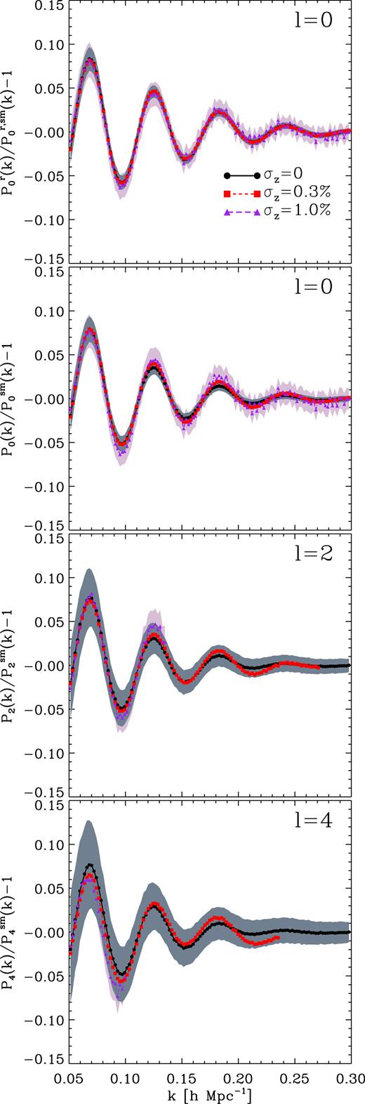
In the top panels of Fig. 1 we display the average power spectrum moments from our analytic expression and from the COLA ensemble. Symbols and colours indicate the results for samples with different number densities and photo-z errors, as stated in the legend. To compute our model, we employ the average |$P^r_0$| from the COLA ensemble with n = 0.03 h³ Mpc⁻³ and σ_|$v$| = 3 × 10⁻⁴, where σ_|$v$| is obtained by fitting our analytic model to power spectrum moments of samples without photo-z errors.

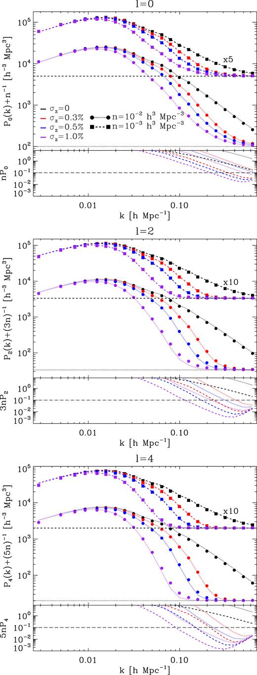
Top panels: impact of photo-z errors on P0, P2, and P4. Symbols show the average results from an ensemble of 1 000 N-body simulations and lines our analytic predictions (equations 10–14), which employ as input the average $P^r_0$ from simulations with n = 0.03 h3 Mpc−3 and σ$v$ = 3 × 10−4. The colour and shape of lines and symbols indicate the size of Gaussian photo-z errors and the number density for each sample, respectively, as stated in the legend. Results for different number densities are vertically displaced for clarity. We employ this colour-coding in what follows. Horizontal lines indicate the shot noise level. Our analytic model precisely captures the effect of photo-z errors. Bottom panels: ratio of shot noise corrected power spectrum moments from simulations and shot noise. On the scales where (2ℓ + 1)nPℓ < 0.1 (indicated by long-dashed lines) the shot noise correction is no longer accurate.

Figure 1.

Top panels: impact of photo-z errors on P₀, P₂, and P₄. Symbols show the average results from an ensemble of 1 000 N-body simulations and lines our analytic predictions (equations 10–14), which employ as input the average |$P^r_0$| from simulations with n = 0.03 h³ Mpc⁻³ and σ_|$v$| = 3 × 10⁻⁴. The colour and shape of lines and symbols indicate the size of Gaussian photo-z errors and the number density for each sample, respectively, as stated in the legend. Results for different number densities are vertically displaced for clarity. We employ this colour-coding in what follows. Horizontal lines indicate the shot noise level. Our analytic model precisely captures the effect of photo-z errors. Bottom panels: ratio of shot noise corrected power spectrum moments from simulations and shot noise. On the scales where (2ℓ + 1)nP_ℓ < 0.1 (indicated by long-dashed lines) the shot noise correction is no longer accurate.

Open in new tab Download slide

We can see that our numerical and analytical results show good agreement. The discrepancies, of the order of |$10\, \hbox{ per cent}$|⁠, arise from the inaccuracy of our RSD model and shot noise subtraction. In the bottom panels of Fig. 1, we display the ratio of shot noise corrected moments and their shot noise level. The long dashed line indicates when the shot noise level is 10 times greater than the amplitude of shot noise corrected moments. As we can see, below this line the shot noise subtraction is no longer precise.

Overall, we can see that photo-z errors suppress the amplitude of P₀, P₂, and P₄ for all wavenumbers, specially on small scales. The Poisson noise, however, is unaltered. Therefore, for a given number density of objects, photo-zs reduce the number of modes and scales useful for cosmological analyses. This is the main effect for galaxy clustering.

3.2 Variance of power spectrum moments

3.2.1 General expressions

The effect of photo-z errors is not only to modify the amplitude of the power spectrum P but also its Gaussian covariance. Let us first consider the diagonal elements of the power spectrum covariance matrix:

\begin{eqnarray*} \sigma^2[P](k) = \frac{2}{N_k} \sum_{\boldsymbol{k}_i} \langle |\hat{\delta }(\boldsymbol{k}_i)|^4\rangle - \langle \hat{P}(\boldsymbol{k}_i) \rangle^2, \end{eqnarray*}

(15)

where ⟨...⟩ denotes the ensemble average over multiple realizations/universes. Factor 2 appears because only half of the modes of the power spectrum are independent due to the reality of |$\delta (\boldsymbol{x})$|⁠.

Assuming that the real and imaginary parts of |$\hat{\delta }(\boldsymbol{k})$| are Gaussian random variables with zero mean and standard deviation P/2, and combining equations (10) and (15), we obtain the following expression for the variance of power spectrum moments in redshift space under the presence of shot noise, photo-z errors, and small-scale velocities:

\begin{eqnarray*} \sigma^2[P_\ell ] &=& \frac{2}{N_k} \biggl [\langle \mu^{2\ell }{\cal F}^4\rangle_{\hat{\boldsymbol{k}}} +\frac{2\langle \mu^{2\ell } {\cal F}^2\rangle_{\hat{\boldsymbol{k}}}}{n P^r_0}\nonumber\\&& \quad +\, \frac{1}{(2\ell +1)(n P^r_0)^2}\biggr ](P^r_0)^2, \end{eqnarray*}

(16)

where this expression reduces to that provided by Colombi et al. (2009) for ℓ = 0 in real space without photo-z errors (⁠|${\cal F}= 1$|⁠). Note that to compute the diagonal terms of the covariance between two power spectrum moments P_ℓ and |$P_{\ell^{\prime }}$|⁠, we only have to substitute 2ℓ by ℓ + ℓ^΄ in the previous equation.

Note that for a Gaussian |$\Pr [\delta r_z]$|⁠, all terms in equation (16) have an analytic expression, which we provided in Section 3.1.2. We can thus analytically compute the variance of any power spectrum moment.

3.2.2 Comparison with simulations: diagonal terms

In Fig. 2 we display the variance of P₀, P₂, and P₄ for the same samples shown in Fig. 1. In the bottom panels we compare our analytic model and the results from our simulations. Overall, our expressions correctly capture the effect of photo-zs – the agreement is to within |$5\, \hbox{ per cent}$|⁠, |$10\, \hbox{ per cent}$|⁠, and |$20\, \hbox{ per cent}$| for P₀, P₂, and P₄, respectively. The differences originate from assuming that the matter density field is Gaussian, and thus from neglecting in our calculations the contribution of a non-zero trispectrum.

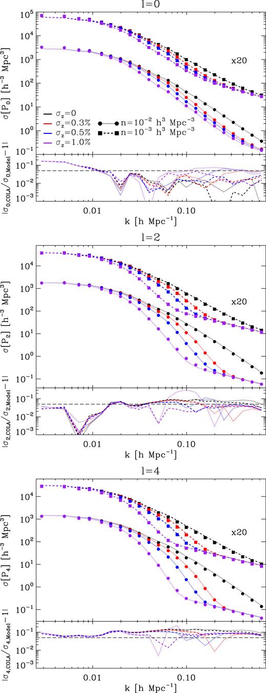
$The impact of photometric errors on the variance of the moments of the redshift-space power spectrum. In each panel we show three sets of curves displaying the results for different number densities. Within each set, colours indicate different redshift uncertainties, as indicated by the legend. Symbols indicate the mean values from our ensemble of simulations, whereas dotted lines indicate the analytic model of equation (16). The bottom panel of each figure shows the fractional difference between our numerical and analytic results.$

Figure 2.

The impact of photometric errors on the variance of the moments of the redshift-space power spectrum. In each panel we show three sets of curves displaying the results for different number densities. Within each set, colours indicate different redshift uncertainties, as indicated by the legend. Symbols indicate the mean values from our ensemble of simulations, whereas dotted lines indicate the analytic model of equation (16). The bottom panel of each figure shows the fractional difference between our numerical and analytic results.

Open in new tab Download slide

We see that photo-z errors reduce the variance, especially on intermediate scales where BAO are located, which is analogous to their effect on the amplitude of power spectrum moments. On the other hand, at a fixed scale, the contribution of shot noise progressively dominates as the order of the moment increases. We can understand this from equation 16: since the last term in brackets of equation does not depend on photo-z errors, it will be more important as the redshift uncertainty increases.

3.2.3 Comparison with simulations: off-diagonal terms

In Fig. 3 we display the diagonal and off-diagonal elements of the auto-correlation matrices of P₀, P₂, and P₄, and their cross-correlations for σ_z = 0 and |$0.5\, \hbox{ per cent}$|⁠. The results shown are computed using 1 000 samples from the COLA ensemble with n = 0.01 h³ Mpc⁻³. The top panels display the cross-correlation between different moments, which is scale-independent for samples with no errors. However, for samples with photo-z errors, they decrease by increasing the value of k. This is the consequence of photo-z errors modifying the information content of power spectrum moments, we further analyse this in the following section.

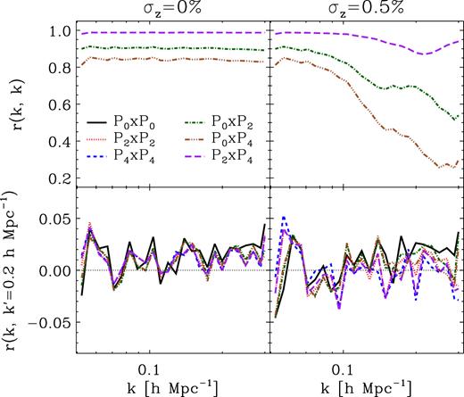
$Diagonal and off-diagonal elements (top and bottom panels, respectively) of the auto-correlation matrices of P0, P2, P4, and their cross-correlations. The left-hand and right-hand panels show the results for σz = 0 and $0.5\, \hbox{ per cent}$, respectively, which are computed using 1 000 samples from the COLA ensemble with n = 0.01 h3 Mpc−3. For samples with photo-z errors the diagonal terms of the cross-correlations decrease on small scales (we do not display those of the auto-correlations because their value is one by definition). Off-diagonal terms are computed at k = 0.2 h Mpc−1, and their amplitudes are small independently of the size of photo-z errors.$

Figure 3.

Diagonal and off-diagonal elements (top and bottom panels, respectively) of the auto-correlation matrices of P₀, P₂, P₄, and their cross-correlations. The left-hand and right-hand panels show the results for σ_z = 0 and |$0.5\, \hbox{ per cent}$|⁠, respectively, which are computed using 1 000 samples from the COLA ensemble with n = 0.01 h³ Mpc⁻³. For samples with photo-z errors the diagonal terms of the cross-correlations decrease on small scales (we do not display those of the auto-correlations because their value is one by definition). Off-diagonal terms are computed at k = 0.2 h Mpc⁻¹, and their amplitudes are small independently of the size of photo-z errors.

Open in new tab Download slide

On the bottom panels we display the off-diagonal terms of the correlation matrices at k = 0.2 h Mpc⁻¹. They are negligible at this scale for samples with and without photo-z errors. This is because photo-z errors do not modify the structure of the covariance matrix. In particular, in the plane-parallel approximation if the real-space power spectrum covariance matrix is diagonal for samples with no photo-z errors, then so it is in redshift space with or without photo-z errors. We check that in the whole range of scales used for BAO analyses in Section 6 off-diagonal are also smaller than |$5\, \hbox{ per cent}$|⁠, which will justify the employment of equation (33). Nonetheless, on even smaller scales the covariance matrix is no longer diagonal due to non-linearities.

3.3 Signal-to-noise ratio

Let us now consider the SNR of power spectrum moments, which we define as the ratio between a given moment and the square root of its variance. We use this approximation because the covariance matrices of P₀, P₂, and P₄ are mostly diagonal on the scales where BAO are located, as we showed in the previous section. Photo-z errors decrease the amplitude of power spectrum moments as well as their variances, and thus the resulting SNR will depend on a balance between both effects.

3.3.1 Toy model

In this subsection we introduce a toy model to understand how photo-z errors modify the SNR of P₀, where it is straightforward to extend this model to ℓ > 0. The model is the following:

\begin{eqnarray*} {\hat{P}}_0 = \frac{1}{2} {\hat{P}}_0^r \left[\eta (\mu_1){\rm e}^{-k^2 \sigma_{\rm eff}^2 \mu_{1}^2}+\eta (\mu_2) {\rm e}^{-k^2 \sigma_{\rm eff}^2 \mu_2^2}\right], \end{eqnarray*}

(17)

where the terms in brackets provide the angular contribution at only two μ-values (μ₁ and μ₂), the symbol |${\hat{P}}_0^r$| denotes the measured real-space ℓ = 0 moment, and η(μ) describes the contribution of large-scale RSDs in a μ-bin. We will assume that μ₁ < μ₂, and thus η(μ₁) < η(μ₂) since on linear scales η(μ) is a monotonically increasing function of μ.

For an ensemble average over a given k-bin we have that the SNR per radial k-interval reads:

\begin{eqnarray*} {\rm SNR} = \frac{1+\eta_{21}\exp (-k^2\, \sigma_{\rm eff}^2\, \Delta \mu^2)}{\sqrt{1+\eta_{21}^2\exp (-2\,k^2\, \sigma_{\rm eff}^2\, \Delta \mu^2)}}, \end{eqnarray*}

(18)

with |$\Delta \mu^2 = \mu_2^2- \mu_1^2$| and η₂₁ = η(μ₂)/η(μ₁). From this expression, we shall consider three different cases:

No photo-z errors nor small-scale RSDs, k σ_eff = 0. In this case
\begin{eqnarray*} {\rm SNR} = \frac{1+\eta_{21}}{\sqrt{1+\eta_{21}^2 }}, \end{eqnarray*}
(19)
where the SNR is always below |$\sqrt{2}$|⁠, which is the value corresponding to real space.
Very large photo-z errors, k σ_eff → ∞. In this limit, the value of the SNR is 1. It is smaller than that in the first case because all information along k-modes parallel to the LOS is lost.
Small photo-z errors, k σ_eff → 0. In this case, to first order in (k σ_eff)², we obtain
\begin{eqnarray*} {\rm SNR} &=& \frac{1+\eta_{21}}{\sqrt{1+\eta_{21}^2}} +\frac{\Delta \mu^2\, \eta_{21}\,(\eta_{21}-1)}{(1+\eta_{21}^2)^{3/2}}\nonumber\\&&\times \,(k\, \sigma_{\rm eff})^2 +{\cal O}\bigl [(k\, \sigma_{\rm eff})^4\bigr ], \end{eqnarray*}
(20)
where in this limit the SNR increases with respect to the case without photo-z errors nor small-scale RSDs as η₂₁ > 1. This behaviour must thus yield a local maximum in the SNR, since for larger k σ_eff values we must recover the second case. This reflects that in this limit photo-z errors affect more the standard deviation of P₀ than its amplitude, and thus they slightly increase the SNR.

From equation (18) we find that the scale corresponding to the local maximum of the SNR, |$\partial ({\rm SNR}) / \partial (k\, \sigma_{\rm eff})^2 = 0$|⁠, is (k σ_eff)² = ln(η₂₁)/Δμ². That is (k σ_eff)² ≃ 1, as shown in the top panel of Fig. 4.

Ratio of the SNR of power spectrum moments, Pℓ/σ[Pℓ], to that of a case with no photo-z errors and n = 0.03 h3 Mpc−3 in real space, Pr/σ[Pr]. On large scales, the SNR of Pℓ is greater for samples with a large number of densities and photo-z errors. However, on small scales the SNR of power spectrum moments decreases by increasing σz.

Figure 4.

Ratio of the SNR of power spectrum moments, P_ℓ/σ[P_ℓ], to that of a case with no photo-z errors and n = 0.03 h³ Mpc⁻³ in real space, P^r/σ[P^r]. On large scales, the SNR of P_ℓ is greater for samples with a large number of densities and photo-z errors. However, on small scales the SNR of power spectrum moments decreases by increasing σ_z.

Open in new tab Download slide

3.3.2 Comparison with simulations

We now compare our analytic expressions for the SNR of power spectrum moments (i.e. those derived in the previous two subsections) with the results from the COLA ensemble. In Fig. 4 we show the SNR of P₀, P₂, and P₄ relative to that of the real-space power spectrum with n = 0.03 h³ Mpc⁻³ and no photo-z errors. We present the redshift-space results for two number densities, as indicated by the legend. In all cases we can see that our model, indicated by lines, approximately reproduces the numerical data, displayed by symbols. The differences for n = 10⁻²h³ Mpc⁻³ on large scales are driven by our model for the shot noise subtraction. Independently of the size of photo-z errors, on large scales the SNR of each moment is lower than that of the real-space power spectrum. This implies that, in the regime where shot noise is subdominant and despite the clustering enhancement due to large-scale RSD, in redshift space the SNR of power spectrum moments is lower than that in real space. This confirms the predictions of the toy model introduced in the previous section.

For samples with photo-z errors, we appreciate an increase in the SNR relative to the case with no photo-z errors on scales where k σ_eff ≃ 1, and a decrease on scales where the contribution of shot noise is the dominant in equation (16). Moreover, for |$\sigma_z \lesssim 0.5\, \hbox{ per cent}$|⁠, the enhancement occurs on the scales where BAO are located. As BAOs are suppressed by the non-linear evolution of the matter density field and RSD, this enhancement could imply that stronger cosmological constraints are derived from samples with sub-percent photo-z errors. We will return to this in the next section. Note that these apparent advantages may disappear after applying reconstruction procedures to the density field.

In Table 1 we show the ratio between the total SNR of P₀, P₂, and P₄ (computed taking into account the covariances among them; see Fig. 3) and that of the real-space power spectrum with no photo-z errors and n = 0.03 h³ Mpc⁻³. This ratio, r_SNR, is computed from 0.05 to 0.3 h Mpc⁻¹, the range of scales that we use for BAO analyses in Section 6. We find that r_SNR = 1 for samples with no photo-z errors and n = 10⁻²h³ Mpc⁻³, and thus there is the same amount of information in redshift space as in real space. Nevertheless, this information is no equally distributed in both spaces. In real space and for samples with no photo-z errors all the information is stored in the ℓ = 0 moment, whereas in redshift space it is distributed between the ℓ = 0, 2, and 4 moments. In this case, we find that the ℓ = 0 moment accounts for |${\simeq } 97\, \hbox{ per cent}$| of the signal, the ℓ = 2 moment the remaining |${\simeq } 3\, \hbox{ per cent}$|⁠, and the ℓ = 4 moment does not contain any new information. Examining samples with a lower number density we find that the ℓ = 0 moment encodes even more information, whereas P₄ starts to provide as much information as P₂. This motivates the analysis of P₀, P₂, and P₄ in Section 6.

Table 1.

Open in new tab

Ratio of the total SNR of P₀, P₂, and P₄ and the SNR of the real-space power spectrum with no photo-z errors and n = 0.03 h³ Mpc⁻³. This ratio is computed from 0.05 to 0.3 h Mpc⁻¹, the range of scales used for BAO analyses in Section 6.

n [h³ Mpc⁻³]	\|$\sigma_z\,[\hbox{per cent}]$\|	\|$r_{\rm SNR}=\frac{{\rm SNR}[\sigma_z]}{{\rm SNR}_r[\sigma_z=0]}$\|
10⁻²	0	1.00
10⁻²	0.3	0.61
10⁻²	0.5	0.52
10⁻²	1.0	0.39
10⁻³	0	0.70
10⁻³	0.3	0.40
10⁻³	0.5	0.31
10⁻³	1.0	0.22
10⁻⁴	0	0.21
10⁻⁴	0.3	0.11
10⁻⁴	0.5	0.08
10⁻⁴	1.0	0.05

n [h³ Mpc⁻³]	\|$\sigma_z\,[\hbox{per cent}]$\|	\|$r_{\rm SNR}=\frac{{\rm SNR}[\sigma_z]}{{\rm SNR}_r[\sigma_z=0]}$\|
10⁻²	0	1.00
10⁻²	0.3	0.61
10⁻²	0.5	0.52
10⁻²	1.0	0.39
10⁻³	0	0.70
10⁻³	0.3	0.40
10⁻³	0.5	0.31
10⁻³	1.0	0.22
10⁻⁴	0	0.21
10⁻⁴	0.3	0.11
10⁻⁴	0.5	0.08
10⁻⁴	1.0	0.05

Table 1.

Open in new tab

Ratio of the total SNR of P₀, P₂, and P₄ and the SNR of the real-space power spectrum with no photo-z errors and n = 0.03 h³ Mpc⁻³. This ratio is computed from 0.05 to 0.3 h Mpc⁻¹, the range of scales used for BAO analyses in Section 6.

n [h³ Mpc⁻³]	\|$\sigma_z\,[\hbox{per cent}]$\|	\|$r_{\rm SNR}=\frac{{\rm SNR}[\sigma_z]}{{\rm SNR}_r[\sigma_z=0]}$\|
10⁻²	0	1.00
10⁻²	0.3	0.61
10⁻²	0.5	0.52
10⁻²	1.0	0.39
10⁻³	0	0.70
10⁻³	0.3	0.40
10⁻³	0.5	0.31
10⁻³	1.0	0.22
10⁻⁴	0	0.21
10⁻⁴	0.3	0.11
10⁻⁴	0.5	0.08
10⁻⁴	1.0	0.05

n [h³ Mpc⁻³]	\|$\sigma_z\,[\hbox{per cent}]$\|	\|$r_{\rm SNR}=\frac{{\rm SNR}[\sigma_z]}{{\rm SNR}_r[\sigma_z=0]}$\|
10⁻²	0	1.00
10⁻²	0.3	0.61
10⁻²	0.5	0.52
10⁻²	1.0	0.39
10⁻³	0	0.70
10⁻³	0.3	0.40
10⁻³	0.5	0.31
10⁻³	1.0	0.22
10⁻⁴	0	0.21
10⁻⁴	0.3	0.11
10⁻⁴	0.5	0.08
10⁻⁴	1.0	0.05

The results of Table 1 indicate that the value of r_SNR decreases by increasing the size of photo-z errors. This is somewhat expected, as we can see in Fig. 4 that the increment in the SNR for samples with photo-z errors only occurs on large scales, whereas on small scales the SNR is reduced.

4 EFFECT OF PHOTOMETRIC REDSHIFT ERRORS ON BAO

In this section we investigate the effect of photo-z errors on the BAO feature imprinted in power spectrum moments. In Section 4.1 we study the suppression of BAOs due to the combined effect of photo-z errors, the non-linear evolution of the matter density field, and RSD. In Section 4.2 we analyse the cosmological information encoded in BAOs, in Section 4.3 we introduce a model to estimate the uncertainty in measuring the BAO scale, and in Section 4.4 we address how to extract cosmological information from the joint analysis of power spectrum moments.

4.1 The shape of the BAO signal

Let us begin by considering the following quantity:

\begin{eqnarray*} B_\ell (k) \equiv \frac{P_\ell (k)}{P_\ell^{\rm sm}(k)} - 1, \end{eqnarray*}

(21)

where |$P_\ell^{\rm sm}$| is a no-wiggle version of P_ℓ. This is a quantity with the same broad-band shape as P_ℓ but no BAO. Therefore, B_ℓ is insensitive to the overall shape of the observed moments and isolates the BAO wiggles.

Motivated by Renormalized Perturbation Theory (Crocce & Scoccimarro 2008), we write the non-linear redshift-space power spectrum as

\begin{eqnarray*} P(k, \mu ) = \left[P_{\rm lin}(k)\,G(k, \mu ) + P_{\rm mc}(k, \mu ) \right]\,b^2\, {\cal F}^2, \end{eqnarray*}

(22)

where P_lin is the linear theory power spectrum in real space, P_mc denotes contribution of the coupling between different k-modes, and G is a propagator that controls the suppression of BAOs due to non-linearities and RSD. This propagator is well approximated by a 2D exponential function:

\begin{eqnarray*} G(k, \mu ) = \exp \left\lbrace -\left[ (1 - \mu^2)\,k^2\, \sigma^2_{\perp } + \mu^2\,k^2 \sigma^2_{\parallel }\right] \right\rbrace , \end{eqnarray*}

(23)

where σ|$_{\parallel}$| and σ_⊥ are parameters that control the suppression of k-modes along and perpendicular to the LOS, respectively. Note that, in redshift space σ|$_{\parallel}$| > σ_⊥. This is a consequence of peculiar velocities and the non-linear mapping between real and redshift-space positions, and it implies that the larger the value of μ, the greater the suppression of BAO for a given wavemode (e.g. Seo & Eisenstein 2007; Sánchez, Baugh & Angulo 2008).

Let us now write a theoretical model for B_ℓ:

\begin{eqnarray*} B_\ell (k) \simeq B_{\rm lin}(k)\,G_{\rm eff, \ell }(k), \end{eqnarray*}

(24)

where |$B_{\rm lin}=P_{\rm lin}/P^{\rm sm}_{\rm lin}-1$|⁠, and

\begin{eqnarray*} G_{\rm eff, \ell }(k) = \frac{\langle G(k, \mu )\, \mu^\ell \, {\cal F}^2\rangle_{\hat{\boldsymbol{k}}}}{\langle \mu^\ell \, {\cal F}^2\rangle_{\hat{\boldsymbol{k}}}}, \end{eqnarray*}

(25)

In deriving these expressions, we have assumed that |$P\simeq [P_{\rm lin}^{\rm sm} + (P_{\rm lin}-P_{\rm lin}^{\rm sm})G]b^2{\cal F}^2$| and |$P^{\rm sm}\simeq P_{\rm lin}^{\rm sm} b^2{\cal F}^2$|⁠. These assumptions are not strictly correct because they do not take into account the P_mc term in equation (22), and thus equation (25) does not predict a shift in the BAO scale due to non-linearities as the full model does (Crocce & Scoccimarro 2008).

The term G_{eff, ℓ} gives the effective suppression of BAOs in P_ℓ, as a function of the scale. As we can see, this quantity is a weighted average of G(k, μ), where the weights are given by photo-z errors and RSD. Therefore, a balance between these two aspects will determine the final appearance of BAOs, as we will see next.

4.1.1 The Gaussian case and comparison with simulations

In the particular case of Gaussian photo-z errors, G_{eff, ℓ} has an analytic expression. In the top, middle, and bottom panels of Fig. 5, we show G_{eff, 0}, G_{eff, 2}, and G_{eff, 4}, respectively. To build this figure, we used σ|$_{\parallel}$| = 6.8 h⁻¹ Mpc and σ_⊥ = 4.3 h⁻¹ Mpc (these values were set by our fits to the numerical simulations presented in Section 6). The vertical dotted and dashed lines indicate the scale at which the suppression of BAO is |$50\, \hbox{ per cent}$| and |$90\, \hbox{ per cent}$|⁠, respectively.

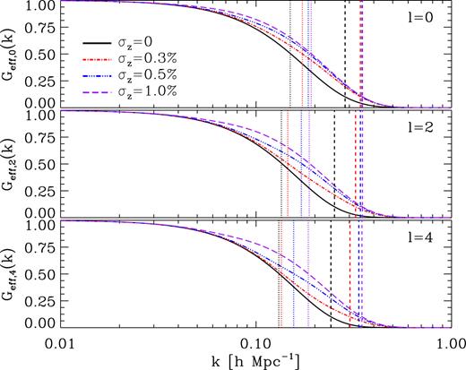
Suppression of BAOs due to the combined effect of photo-z errors, non-linearities, and RSD. The top, middle, and bottom panels show the results for P0, P2, and P4, respectively. Dotted and dashed lines indicate when the suppression is greater than a factor of 2 and 10, respectively. The suppression of BAOs is weaker for samples with photo-z errors because they decrease the weight of k-modes parallel to the LOS in the angular average, where in redshift space these modes are more suppressed than the perpendicular ones owing to RSD.

Figure 5.

Suppression of BAOs due to the combined effect of photo-z errors, non-linearities, and RSD. The top, middle, and bottom panels show the results for P₀, P₂, and P₄, respectively. Dotted and dashed lines indicate when the suppression is greater than a factor of 2 and 10, respectively. The suppression of BAOs is weaker for samples with photo-z errors because they decrease the weight of k-modes parallel to the LOS in the angular average, where in redshift space these modes are more suppressed than the perpendicular ones owing to RSD.

Open in new tab Download slide

As we can see, the BAO suppression is weaker for samples with larger photo-z errors. This has an interesting consequence, photo-z errors make BAO wiggles to appear sharper. Furthermore, for a given photo-z error, the suppression is stronger for higher order moments. This counter-intuitive result can be understood by recalling that LOS modes – where BAO smearing is more significant – contribute less to a given moment, thus, when photo-z are included, BAOs appear more alike to the less-damped real-space case.

In order to check the accuracy of the predictions of equation (25), we measure B from the COLA ensemble. To obtain the no-wiggle power spectrum |$P_\ell^{\rm sm}$|⁠, we fit P_ℓ using the following model:

\begin{eqnarray*} P_{\rm fit, \ell }(k) &=& A_{0, \ell } \langle \mu^\ell \, {\cal F}^2\rangle_{\hat{\boldsymbol{k}}} P_{\rm nw}(k) + A_{1, \ell } k^2 + A_{2, \ell } k \nonumber\\ && + A_{3, \ell }+\, A_{4, \ell } k^{-1} + A_{5, \ell } k^{-2} + A_{6, \ell } k^{-3}, \end{eqnarray*}

(26)

where P_nw is the non-wiggle power spectrum from (Eisenstein & Hu 1998), and the factors A_{i, ℓ} give us enough freedom to fit the broad-band shape of P_ℓ without fitting the oscillations. We explicitly show this in Fig. 6, where we display the average value of B measured from samples of the COLA ensemble with n = 10⁻² h³ Mpc⁻³. In descending order, the panels show the results for |$P^r_0$|⁠, P₀, P₂, and P₄. Note that for samples with sub-percent photo-z errors, B₂ and B₄ are not displayed up to k ∼ 0.3 h Mpc⁻¹. This is because on small scales the measurements start to be progressively dominated by shot noise.

$Average Bℓ computed using 1 000 samples from the COLA ensemble with n = 0.01 h3 Mpc−3 for $P^r_0$, P0, P2, and P4. The grey and purple areas denote the 1σ confidence region for samples with σz = 0 and $1\, \hbox{ per cent}$, respectively. For samples with photo-z errors we do not show the results up to k ∼ 0.3 h Mpc−1 because our procedure for extracting Bℓ does not work well on scales where power spectrum moments are dominated by shot noise. In real space the amplitude of BAO is not modified by photo-z errors, whereas in redshift space it grows with their size. This confirms the predictions of Fig. 5.$

Figure 6.

Average B_ℓ computed using 1 000 samples from the COLA ensemble with n = 0.01 h³ Mpc⁻³ for |$P^r_0$|⁠, P₀, P₂, and P₄. The grey and purple areas denote the 1σ confidence region for samples with σ_z = 0 and |$1\, \hbox{ per cent}$|⁠, respectively. For samples with photo-z errors we do not show the results up to k ∼ 0.3 h Mpc⁻¹ because our procedure for extracting B_ℓ does not work well on scales where power spectrum moments are dominated by shot noise. In real space the amplitude of BAO is not modified by photo-z errors, whereas in redshift space it grows with their size. This confirms the predictions of Fig. 5.

Open in new tab Download slide

We find that in real space the BAO feature is the identical in the cases with and without photo-z errors. This is expected from equation (25), as in real space σ|$_{\parallel}$| = σ_⊥, and thus |$G_{\rm eff,0} = e^{-(k\, \sigma_\perp )^2}$|⁠. However, in redshift space, BAOs are less suppressed for samples with greater photo-z errors, confirming the predictions of Fig. 5 and our analytic model.

4.2 Cosmological information encoded in BAO

We now explore the cosmological information encoded in the BAO feature. Let us consider a given scale |$k = \sqrt{k_{\parallel }^2 + k_{\perp }^2}$| and angle μ = k|$_{\parallel}$|/k in the two-dimensional power spectrum. Assuming a fiducial cosmology, they are observed as

\begin{eqnarray*} k^{\rm fid} = k/\alpha \equiv k\sqrt{\mu^2 \alpha_\parallel^{-2} + (1-\mu^2) \alpha_\perp^{-2}}, \end{eqnarray*}

(27)

\begin{eqnarray*} \mu^{\rm fid} = \epsilon \mu \equiv \frac{\mu }{\sqrt{\mu^2+(1-\mu^2)(\alpha_\parallel /\alpha_\perp )^2}}, \end{eqnarray*}

(28)

where |$\alpha_{\parallel }\equiv \frac{H^{\rm fid}(z)r_{\rm s}^{\rm fid}}{H(z)r_{\rm s}}$| and |$\alpha_{\perp }\equiv \frac{D_{\rm A}(z)r_{\rm s}^{\rm fid}}{D^{\rm fid}_{\rm A}(z)r_{\rm s}}$|⁠. In the above expressions, r_s is the sound horizon scale, D_A is the angular diameter distance, H is the Hubble parameter, and fid denotes these quantities in the fiducial cosmology. The observed redshift-space power spectrum moments are thus

\begin{eqnarray*} P_\ell (k/\alpha_{\ell }) &=& \alpha_\parallel^{-1} \alpha_\perp^{-2} \big\langle \epsilon^{\ell +1} \mu^\ell \left[1+\epsilon^2\mu^2\left(\alpha_\parallel^2 \alpha_\perp^{-2}-1\right)\right] \nonumber\\ &&\quad\times \,\mathcal {F}^2(k/\alpha , \epsilon \mu ) P_0^r(k/\alpha ) \big\rangle_{\hat{\boldsymbol{k}}}, \end{eqnarray*}

(29)

where assuming an incorrect cosmology would cause isotropic and anisotropic deformations. For the full expression of deformations in observed multipoles, see Padmanabhan & White (2008) in Fourier space and Xu et al. (2013) in configuration space.

Since here we are mostly interested in the information encoded in the BAO scale, we follow Ross, Percival & Manera (2015, R15 hereafter) and focus only on the stretch parameters α_ℓ as a function of α|$_{\parallel}$| and α_⊥.¹ As in R15, we will also assume that the information on α_ℓ is separable from the overall shape of power spectrum moments and that the information in different μ bins is independent. Under these assumptions,

\begin{eqnarray*} \alpha_\ell (k) = \frac{\left\langle \, \mu^\ell \, {\cal F}^2 \alpha \right\rangle_{\hat{\boldsymbol{k}}}}{\langle \mu^\ell {\cal F}^2 \rangle_{\hat{\boldsymbol{k}}}}, \end{eqnarray*}

(30)

where the scale dependence of α_ℓ emerges from the scale dependence of |${\cal F}^2$|⁠. The previous expression reduces to equation (6) of R15 for samples with no photo-z errors nor small-scale RSD. Therefore, small-scale RSD and/or photo-z errors induce a scale dependence in the stretch parameter.

As in R15, we find that the first-order expansion of α_ℓ around the fiducial solution can be expressed as |$\alpha_\ell (k) = \alpha^{m_\ell (k)}_{\parallel } \alpha^{n_\ell (k)}_{\perp }$|⁠, where m_ℓ and n_ℓ are given by

\begin{eqnarray*} m_\ell (k) \equiv \left. \frac{\partial \left\langle \alpha_\ell \right\rangle }{\partial \alpha_{\parallel }}\right|_{\alpha_\parallel =\alpha_\perp =1} = \frac{\langle \mu^{\ell +2} {\cal F}^2 \rangle_{\hat{\boldsymbol{k}}}}{\langle \mu^\ell {\cal F}^2 \rangle_{\hat{\boldsymbol{k}}}}, \end{eqnarray*}

(31)

\begin{eqnarray*} n_\ell (k) \equiv \left. \frac{\partial \left\langle \alpha_\ell \right\rangle }{\partial \alpha_{\perp }}\right|_{\alpha_\parallel =\alpha_\perp =1} =1- m_\ell (k), \end{eqnarray*}

(32)

where the higher the value of m_ℓ, the more sensitive α_ℓ is to the Hubble parameter. For the case of Gaussian photo-z errors, m_ℓ and n_ℓ have analytic expressions.

Going back to the stretch parameter, the known case with m₀ = 1/3 and n₀ = 2/3 (Eisenstein et al. 2005) is only recovered in real space without photo-z errors. In redshift space, there is a dependence of m_ℓ and n_ℓ on β even if σ_z = 0. In general, the effect of photo-z errors and small-scale RSD is to decrease the sensitivity of α_ℓ on H, whereas large-scale RSD have the opposite effect. Nonetheless, the exact degeneracy between α|$_{\parallel}$| and α_⊥ also depends on the properties of analysed sample, such as its large-scale bias.

4.3 Toy model for the uncertainty in the stretch parameter

In Section 3.3 we studied the SNR of power spectrum moments and in the previous section we showed that the suppression of the BAO feature depends on G_{eff, ℓ}. In this section we use this to derive an analytic estimation of the uncertainty in α_ℓ as a function of large-scale bias, number density, photo-z error, and cosmology.

To build an estimator for the precision measuring α_ℓ, we will assume that its uncertainty is given by the convolution of the one measuring P_ℓ and the amplitude of BAO wiggles in P_ℓ. The latter obviously depends on the suppression of BAO due to non-linearities and RSD, which as we explained before is captured by G_{eff, ℓ}. For conventional approaches using Fisher matrix forecast, see for instance Seo & Eisenstein (2003).

We estimate the amplitude of unsuppressed BAOs in linear theory by measuring the absolute value of the local extrema of 1 + B_lin. Then, we do a linear fit of these values, B_amp. The product of this quantity and equation (25), G_{eff, ℓ} B_amp, gives thus the maximum amplitude of BAO wiggles in P_ℓ under the presence of non-linearities, RSD, and photo-z errors.

In BAO analyses, the stretch parameter α_ℓ is extracted from an interval of scales. As this parameter is scale-dependent due to small-scale velocities and photo-z errors, it is useful to define an effective stretch parameter α_{eff, ℓ}. We estimate the uncertainty in this parameter as the uncertainty in a moment times the amplitude of BAO wiggles

\begin{eqnarray*} \hat{\sigma }[\alpha_{{\rm eff}, \ell }] &=& \frac{A_\ell }{(k_{\rm max}-k_{\rm min})^c} \nonumber\\&&\times \,\left(\int_{k_{\rm min}}^{k_{\rm max}}\text{d}k\, \frac{P_\ell^2\,G_{\rm eff, \ell }^2\,B_{\rm amp}^2}{\sigma^2[P_\ell ]}\right)^{-0.5}, \end{eqnarray*}

(33)

where A_ℓ and c are free parameters. Note that we assumed that the off-diagonal terms of the covariance matrices of power spectrum moments are negligible on the range of scales where BAOs are located (see Section 3.2.3).

4.4 The scale dependence of cosmological information

In Section 4.2 we showed that there is a scale dependence for the cosmological information encoded in BAOs, which introduces an additional complication while extracting information from BAO analyses. We present in the top, middle, and bottom panels of Fig. 7 the value of m₀, m₂, and m₄ as a function of the scale, respectively. Solid lines indicate the results for different photo-z errors, b = 1, and our adopted cosmology (cf. Section 2.1). Dashed lines denote when the sensitivity of BAOs to the Hubble parameter is the same as in real-space, m = 1/3. As we can see, the higher is the order of the moment, the greater is the sensitivity on the Hubble parameter. For example, if we look at samples with |$\sigma_z=0.3\, \hbox{ per cent}$|⁠, m₀, m₂, and m₄ are greater than 1/3 up to k ≃ 0.1, 0.2, and 0.3 h Mpc⁻¹, respectively. Therefore, the analysis of BAOs in the ℓ = 4 moment of samples with |$\sigma_z=0.3\, \hbox{ per cent}$| is more sensitive to the Hubble parameter than in real space. This highlights the importance of analysing BAOs in the l = 0 and l = 2 moments. In addition, we can see that there is a scale dependence of m_ℓ for samples with no photo-z errors, which is caused by small-scale velocities.

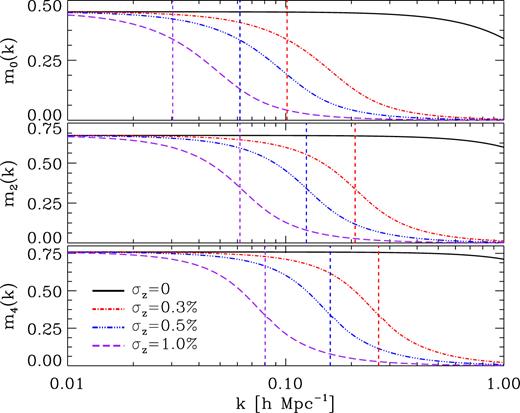
Sensitivity of BAOs to the Hubble parameter as a function of the scale, mℓ. The top, medium, and bottom panels show the results for BAOs in P0, P2, and P4, respectively. The vertical lines indicate the scale at which the dependence of BAO on the Hubble parameter is smaller than for samples with no photo-z errors in real space (m = 1/3). As expected, the larger the photo-z error, the smaller is the dependence of BAOs on the Hubble parameter. We can see that samples with no photo-z errors also present a dependence of mℓ on the scale, which occurs due to small-scale velocities.

Figure 7.

Sensitivity of BAOs to the Hubble parameter as a function of the scale, m_ℓ. The top, medium, and bottom panels show the results for BAOs in P₀, P₂, and P₄, respectively. The vertical lines indicate the scale at which the dependence of BAO on the Hubble parameter is smaller than for samples with no photo-z errors in real space (m = 1/3). As expected, the larger the photo-z error, the smaller is the dependence of BAOs on the Hubble parameter. We can see that samples with no photo-z errors also present a dependence of m_ℓ on the scale, which occurs due to small-scale velocities.

Open in new tab Download slide

We can derive the relation between the precision in measuring α_ℓ and the radial and perpendicular components of α – Hubble parameter and angular diameter distance, respectively – using equations (31) and (32):

\begin{eqnarray*} \sigma^2[\alpha_{\ell , \ell^{\prime }}]=m_\ell^2\, \sigma^2[\alpha_{\parallel }] +n_{\ell^{\prime }}^2\, \sigma^2[\alpha_{\perp }], \end{eqnarray*}

(34)

where the uncertainties in the radial and perpendicular components are σ[α|$_{\parallel}$|] and σ[α_⊥], respectively. Consequently, to extract the precision in measuring both components, we need to perform a joint fit of at least two power spectrum moments.

In the same way that we computed an effective value for the stretch parameter in the previous section, we can now estimate an overall degeneracy between the parallel and perpendicular components of α_ℓ when they are estimated from an interval of scales, m_{eff, ℓ}. To do this, we compute the variance-weighted average of m_ℓ and n_ℓ over the desired k-interval, where the variances are given by equation (33). Explicitly,

\begin{eqnarray*} m_{\rm eff, \ell } =& \frac{\int_{k_{\rm min}}^{k_{\rm max}} \text{d}k\, \frac{m_\ell P_\ell^2 G_{\rm eff, \ell }^2 B_{\rm amp}^2}{\sigma^2[P_\ell ]}}{\int_{k_{\rm min}}^{k_{\rm max}} \text{d}k\, \frac{P_\ell^2 G_{\rm eff, \ell }^2 B_{\rm amp}^2}{\sigma^2[P_\ell ]}}, \end{eqnarray*}

(35)

\begin{eqnarray*} n_{\rm eff, \ell } =& 1-m_{\rm eff, \ell }, \end{eqnarray*}

(36)

and thus, the degeneracy between the overall precision in the parallel and perpendicular components of α_{eff, ℓ} is given by

\begin{eqnarray*} \sigma^2[\alpha_{\rm eff, \ell }]=m_{\rm eff, \ell }^2 \, \sigma^2[\alpha_{\parallel }] +n_{\rm eff, \ell }^2\, \sigma^2[\alpha_{\perp }]. \end{eqnarray*}

(37)

Nevertheless, we are interested in the precision measuring H and D_A. In Section 6 we conduct a joint analysis of BAO in P₀, P₂, and P₄ to compute their uncertainties, as it is required the analysis of at least two moments to break the degeneracy in cosmological information along and perpendicular to the LOS. From now on, we drop the subindex eff for simplicity. In this way,

\begin{eqnarray*} \boldsymbol{\Sigma } = \boldsymbol{M}^+\, {\boldsymbol{E}}\,(\boldsymbol{M}^+)^{\rm T}, \end{eqnarray*}

(38)

\begin{eqnarray*} \boldsymbol{\Sigma } = {\left(\begin{array}{l@{\quad}l}\sigma^2[\alpha_\parallel ] & \sigma [\alpha_{\parallel , \perp }]\\\sigma [\alpha_{\parallel , \perp }] & \sigma^2[\alpha_\perp ]\\\end{array}\right)}, \end{eqnarray*}

(39)

\begin{eqnarray*} \boldsymbol{M} = {\left(\begin{array}{l@{\quad}l}m_0 & n_0 \\m_2 & n_2 \\m_4 & n_4 \\\end{array}\right)}, \end{eqnarray*}

(40)

\begin{eqnarray*} \boldsymbol{E} = & {\left(\begin{array}{l@{\quad}l@{\quad}l}\sigma^2[\alpha_0] & \sigma [\alpha_{0,2}] & \sigma [\alpha_{0,4}] \\\sigma [\alpha_{0,2}] & \sigma^2[\alpha_2] & \sigma [\alpha_{2,4}] \\\sigma [\alpha_{0,4}] & \sigma [\alpha_{2,4}] & \sigma^2[\alpha_4] \\\end{array}\right)}, \end{eqnarray*}

(41)

where |$\boldsymbol{M}^+$| is the pseudoinverse of |$\boldsymbol{M}$| (Moore 1920; Bjerhammar 1951; Penrose 1955), |$\boldsymbol{\Sigma }$| is the covariance matrix of H and D_A, and |$\boldsymbol{E}$| is computed from BAO analysis of power spectrum moments.

5 EXTRACTING INFORMATION FROM BAO

In the previous sections we showed how photo-z errors modify the amplitude of power spectrum moments, their variances, the suppression of BAOs, and the cosmological information encoded in them. In this section we employ all this information to create a model to unbiasedly extract the BAO scale, α, from observational and/or simulated data, even under the presence of photo-z errors. We will employ this model on simulated catalogues in Section 6.

5.1 Modelling power spectrum moments

Based on the expressions provided in Section 4.1, we can write the following four parameter model for power spectrum moments:

\begin{eqnarray*} P_{T, \ell } = P^{\rm sm}_\ell (k) \left[B_{\rm lin}(k/\alpha_\ell ) G_\ell (k/\alpha_\ell , \sigma_{\rm eff}, \sigma_\perp ,f) + 1\right] \end{eqnarray*}

(42)

where |$P^{\rm sm}_\ell$| is computed using the same approach as in Section 4.1, the parameter α_ℓ allows for stretching of the BAO, σ_⊥, and f = σ|$_{\parallel}$|/σ_⊥ control BAO suppression. Photo-z errors enter only through G_ℓ. Note that all these parameters only appear in the expression for B_lin and G_ℓ, and thus they are only constrained by BAO information, i.e. our model extracts cosmological information regardless of the overall shape of the analysed moment.

In the following sections we will not vary σ_eff, we will use the value that corresponds to the photo-zerror introduced in each simulation. This is done to avoid degeneracies between σ_⊥ and σ_eff, as both control the suppression of BAOs. In any case, we checked that the value of α_ℓ and its uncertainty are largely independent of fixing σ_eff or not.

5.2 Parameter likelihood calculation

To extract the information encoded in BAOs, we jointly fit P₀, P₂, and P₄. For this, we assume that the probability of observing |$\boldsymbol{d} = [P_0,P_2,P_4]$| is given by a multivariate Gaussian distribution:

\begin{eqnarray*} \Pr (\boldsymbol{d}|\boldsymbol{\pi }) \propto \exp \left[-\frac{1}{2}\left(\boldsymbol{d} - \boldsymbol{t}\right)^{\rm T} {\boldsymbol {\sf C}}^{-1}\left(\boldsymbol{d} - \boldsymbol{t}\right)\right], \end{eqnarray*}

(43)

where |$\boldsymbol{t}(k, \pi )=[P_{T,0},P_{T,2},P_{T,4}]$|⁠, and |$\pi$| = {α₀, α₂, α₄, σ_⊥, f} denote the five free parameters of our model. The priors on these parameters are assumed to be flat over the range: α_ℓ ∈ [0.75, 1.25] and σ_⊥ ∈ [0.5, 10], and f ∈ [1, 10]. We set the minimum value of f to be 1 because in redshift space the combination of RSD and non-linearities make k-modes along the LOS to be the most suppressed (see Section 4.1). We note that the results do not change if we set wider priors. |${\boldsymbol {\sf C}}^{-1}$| is the data precision matrix of |$\boldsymbol{d}$|⁠, which we compute from the COLA ensemble as described in Section 2.2. The interval of scales considered is k = [0.05−0.30] h Mpc⁻¹.

We sample the posterior probability distribution function of |$\pi$| employing the publicly available code emcee (Foreman-Mackey et al. 2013). This code is an affine invariant MCMC ensemble sampler that has been widely tested and used in multiple scientific studies. We configure the code to analyse |$\boldsymbol{d}$| using a chain of 100 random walkers with 5 000 steps each, and a burn-in phase of 500 steps. We checked that this burn-in phase is sufficient to obtain well-behaved chains.

Additionally, we checked that the standard deviations of the best-fit values from the COLA ensemble are compatible with the uncertainties estimated from the likelihood of each simulated catalogue.

6 RESULTS FROM SIMULATED CATALOGUES

In this section we start by studying the quality of the BAO fitting model introduced in the previous section. Then, we apply this model to simulated catalogues with different photo-z errors and number densities. In addition, we study whether introducing photo-z errors following PDFs different from Gaussian impacts our results. Finally, we present a simple procedure to undo the effect of peculiar velocities on power spectrum moments.

We note that in this section we analyse power spectrum moments computed from DM particles. In principle, this could introduce a shift in the stretch parameter with respect to computing power spectrum moments from haloes/galaxies. However, Angulo et al. (2014) addressed this by measuring the stretch parameter from the real- and redshift-space monopole of galaxies selected by star formation and stellar mass in the Millennium XXL simulation (Angulo et al. 2012), finding no additional shifts with respect to the stretch parameter measured from DM particles. Therefore, we will restrict our analysis to DM particles.

6.1 Quality of our model

In Fig. 8 we show the result of fitting the model introduced in equation (42) to samples from the COLA ensemble with σ_z = 0 and n = 10⁻² h³ Mpc⁻³. Symbols indicate the average value of B_ℓ computed from the COLA ensemble, and lines the average of the best-fit to each mock. We display the results for ℓ = 0, ℓ = 2, and ℓ = 4 in black, red, and blue, respectively, where they are offset for clarity. Shaded areas enclose the 1σ region from mock to mock. In the bottom panel we plot the relative difference between the model and data, where we can see that in all cases the typical deviations are statistically insignificant. In addition, our model reproduces the simulated data to within |$1\, \hbox{ per cent}$| on the scales shown, which is more than enough for the next generation of galaxy surveys. We also checked that we obtain similar results for samples with sub-percent photo-z errors.

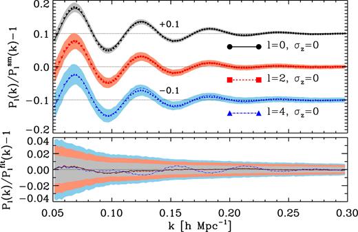
$Relative difference between P0, P2, P4 and their no-wiggle versions for samples with no photo-z errors and n = 10−2 h3 Mpc−3. Symbols and lines display the average results from the COLA ensemble and the average best-fit to each mock using equation (42), respectively. Coloured regions indicate the 1σ region of the scatter from mock to mock. The bottom panel shows the relative difference between the average data and model. The precision of our template is to within $1\, \hbox{ per cent}$, which is greater than the typical scatter from mock to mock.$

Figure 8.

Relative difference between P₀, P₂, P₄ and their no-wiggle versions for samples with no photo-z errors and n = 10⁻² h³ Mpc⁻³. Symbols and lines display the average results from the COLA ensemble and the average best-fit to each mock using equation (42), respectively. Coloured regions indicate the 1σ region of the scatter from mock to mock. The bottom panel shows the relative difference between the average data and model. The precision of our template is to within |$1\, \hbox{ per cent}$|⁠, which is greater than the typical scatter from mock to mock.

Open in new tab Download slide

6.2 Effect of redshift errors

In this section we apply our BAO analysis procedure to power spectrum moments of samples with n = 10⁻²h³ Mpc⁻³ and Gaussian photo-z errors of different sizes.

We start by studying the shift in the stretch parameter with respect to its fiducial value, α_ℓ − 1, from the BAO analysis of real- and redshift-space power spectrum moments of 1 000 samples from the COLA ensemble. In the left-hand and right-hand panels of Fig. 9 we present the distribution of these parameters and their uncertainties, respectively, from the analysis of samples with different photo-z errors. Arrows point to the mean of each distribution, and we gather these values in Table 2. As we can see in the left-hand panels, the average value of α_ℓ − 1 is compatible with zero at the 1σ level for all samples. This implies that for samples with sub-percent photo-z errors our estimator is unbiased relative to the case with no errors. However, for larger photo-z errors this is no longer correct, as we can see for α₄ and |$\sigma_z=1.0\, \hbox{ per cent}$|⁠. This is because our procedure to calculate a smooth version of power spectrum moments does not work well if the amplitude of the moment is of the order of the shot noise level.

Figure 9.

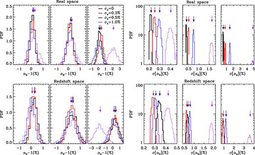
Distribution of α_ℓ (left-hand panels) and their uncertainties (right-hand panels) from MCMC analysis of 1 000 independent catalogues of DM particles with n = 10⁻² h³ Mpc⁻³ and different Gaussian photo-z errors. The precision measuring α_ℓ is computed after marginalizing over the other parameters in the model. The top and bottom rows show the results in real and redshift space, respectively. Arrows point to the mean of each distribution. For samples with sub-percent photo-z errors, the value of α_ℓ is compatible with the fiducial cosmology at the 1σ level (α_ℓ − 1 = 0). Therefore, sub-percent photo-z errors do not introduce an additional shift in the position of BAO. As we can see in the right-hand panels, in real space the precision measuring α_ℓ decreases with the size of photo-z errors. Nevertheless, in redshift space samples with small photo-z errors measure α₀ with more precision than samples with no errors. This is because the suppression of BAO in power spectrum moments decreases with the size of photo-z errors (see Section 4.1).

Open in new tab Download slide

Table 2.

Open in new tab

Average results extracted from the MCMC analysis of 1 000 independent catalogues of DM particles with n = 10⁻²h³ Mpc⁻³. We show the average value of α_ℓ, |$\bar{\alpha }_\ell$|⁠, and the average uncertainty measuring this parameter after marginalising over the other free parameters in the model.

	\|$\bar{\alpha }_0-1\,(\hbox{per cent})$\|	\|$\bar{\alpha }_2-1\,(\hbox{per cent})$\|	\|$\bar{\alpha }_4-1\,(\hbox{per cent})$\|
Real space
0	0.20 ± 0.22	0.23 ± 0.40	0.24 ± 0.52
0.3	0.19 ± 0.25	0.20 ± 0.50	0.44 ± 0.78
0.5	0.14 ± 0.30	0.20 ± 0.78	0.11 ± 1.47
1.0	0.30 ± 0.40	0.29 ± 1.62	2.10 ± 4.81
Redshift space
0	0.32 ± 0.34	0.40 ± 0.68	0.44 ± 0.93
0.3	0.28 ± 0.28	0.34 ± 0.62	0.33 ± 0.93
0.5	0.09 ± 0.31	0.23 ± 0.79	0.18 ± 1.20
1.0	0.09 ± 0.42	0.38 ± 1.92	−1.73 ± 3.62

	\|$\bar{\alpha }_0-1\,(\hbox{per cent})$\|	\|$\bar{\alpha }_2-1\,(\hbox{per cent})$\|	\|$\bar{\alpha }_4-1\,(\hbox{per cent})$\|
Real space
0	0.20 ± 0.22	0.23 ± 0.40	0.24 ± 0.52
0.3	0.19 ± 0.25	0.20 ± 0.50	0.44 ± 0.78
0.5	0.14 ± 0.30	0.20 ± 0.78	0.11 ± 1.47
1.0	0.30 ± 0.40	0.29 ± 1.62	2.10 ± 4.81
Redshift space
0	0.32 ± 0.34	0.40 ± 0.68	0.44 ± 0.93
0.3	0.28 ± 0.28	0.34 ± 0.62	0.33 ± 0.93
0.5	0.09 ± 0.31	0.23 ± 0.79	0.18 ± 1.20
1.0	0.09 ± 0.42	0.38 ± 1.92	−1.73 ± 3.62

Table 2.

Open in new tab

Average results extracted from the MCMC analysis of 1 000 independent catalogues of DM particles with n = 10⁻²h³ Mpc⁻³. We show the average value of α_ℓ, |$\bar{\alpha }_\ell$|⁠, and the average uncertainty measuring this parameter after marginalising over the other free parameters in the model.

	\|$\bar{\alpha }_0-1\,(\hbox{per cent})$\|	\|$\bar{\alpha }_2-1\,(\hbox{per cent})$\|	\|$\bar{\alpha }_4-1\,(\hbox{per cent})$\|
Real space
0	0.20 ± 0.22	0.23 ± 0.40	0.24 ± 0.52
0.3	0.19 ± 0.25	0.20 ± 0.50	0.44 ± 0.78
0.5	0.14 ± 0.30	0.20 ± 0.78	0.11 ± 1.47
1.0	0.30 ± 0.40	0.29 ± 1.62	2.10 ± 4.81
Redshift space
0	0.32 ± 0.34	0.40 ± 0.68	0.44 ± 0.93
0.3	0.28 ± 0.28	0.34 ± 0.62	0.33 ± 0.93
0.5	0.09 ± 0.31	0.23 ± 0.79	0.18 ± 1.20
1.0	0.09 ± 0.42	0.38 ± 1.92	−1.73 ± 3.62

	\|$\bar{\alpha }_0-1\,(\hbox{per cent})$\|	\|$\bar{\alpha }_2-1\,(\hbox{per cent})$\|	\|$\bar{\alpha }_4-1\,(\hbox{per cent})$\|
Real space
0	0.20 ± 0.22	0.23 ± 0.40	0.24 ± 0.52
0.3	0.19 ± 0.25	0.20 ± 0.50	0.44 ± 0.78
0.5	0.14 ± 0.30	0.20 ± 0.78	0.11 ± 1.47
1.0	0.30 ± 0.40	0.29 ± 1.62	2.10 ± 4.81
Redshift space
0	0.32 ± 0.34	0.40 ± 0.68	0.44 ± 0.93
0.3	0.28 ± 0.28	0.34 ± 0.62	0.33 ± 0.93
0.5	0.09 ± 0.31	0.23 ± 0.79	0.18 ± 1.20
1.0	0.09 ± 0.42	0.38 ± 1.92	−1.73 ± 3.62

In real and redshift space the stretch parameter presents a small and positive shift, which is caused by the non-linear evolution of the matter density field (e.g. Angulo et al. 2008; Crocce & Scoccimarro 2008; Smith, Scoccimarro & Sheth 2008; Padmanabhan & White 2009). We also find that this shift slightly decreases with the size of photo-z errors. This is because photo-z errors strongly suppress k-modes along the LOS on small scales, which are the k-modes that present a greater coupling due to non-linearities and RSD, and thus reduce the effective shift in the volume-averaged stretch parameters. Whereas the shifts that we find are statistically significant for the volume of the COLA ensemble, 27 000 h⁻³ Gpc³, for a single simulation they are compatible with zero to within 1σ. Furthermore, these shifts can in principle be approximately corrected for via reconstruction algorithms² (e.g. Eisenstein et al. 2007; Schmittfull et al. 2015) or by recalibrating the estimator employed.

The top-right panel of Fig. 9 displays the uncertainty in the stretch parameter measured from samples in real space. As we expect, the precision measuring |$\alpha^r_\ell$| decreases with the size of photo-z errors. This is the consequence of photo-z errors suppressing the clustering on small scales, which increases the relative contribution of shot noise to the variance, and thus reduces the SNR.

In redshift space the precision measuring α_ℓ is a combination of the effect explained in the previous paragraph and the fact that photo-z errors reduce the overall suppression of BAOs (see Fig. 5). As explained in Section 4.1, they reduce the weight of k-modes parallel to the LOS when doing the angular average of the 3D power spectrum, where these modes are noisier than the perpendicular ones owing to RSD. In the bottom-right panel we can see that the balance between both effects causes σ[α_ℓ] not to be a monotonic function of the size of photo-z errors. We find that α₀ can be measured with more precision from samples with small photo-z errors (⁠|$\sigma_z\le 0.5\, \hbox{ per cent}$|⁠) than from samples with no errors. Nevertheless, if we increase the size of photo-z errors this is no longer true, for instance σ[α₀] for samples with |$\sigma_z=1.0\, \hbox{ per cent}$| is greater than for samples with no photo-z errors. For higher order moments the results are different because the range of scales for which the variance is not dominated by shot noise is smaller. However, for samples with |$\sigma_z= 0.3\, \hbox{ per cent}$| we still find that α₂ and α₄ can be measured with more precision or the same precision, respectively, as from samples with no photo-z errors.

A by-product of the MCMC analysis of power spectrum moments is the value of the parameters (σ_⊥, f), which encode the suppression of the moments perpendicular and parallel to the LOS (σ|$_{\parallel}$| = fσ_⊥), respectively. We find that their average value and uncertainty are approximately the same independently of the size of photo-z errors. For samples with no photo-z errors they are σ_⊥ = 4.02 ± 0.13 and f = 1.06 ± 0.05 in real space, and σ_⊥ = 4.29 ± 0.38 and f = 1.68 ± 0.25 in redshift space. As expected, RSD increase the suppression of k-modes parallel to the LOS: for the COLA ensemble at z = 1 this suppression is |$68\, \hbox{ per cent}$| greater than for k-modes perpendicular to the LOS. This is the main reason behind getting more precise results in α_ℓ from samples in redshift space with sub-percent photo-z errors for which shot noise is not relevant on BAO scales.

6.3 Effect of different PDFs for photometric redshift errors

In general, photo-z errors do not follow a Gaussian PDF. For instance, the comparison between photometric and spectroscopic redshifts in the COSMOS survey shows that the PDF of photo-z errors is well described by a Lorentzian variate (Ilbert et al. 2009). Additionally, for low redshift galaxies the PDF of photo-z errors usually shows a tail towards higher redshifts, which is a natural consequence of imposing z > 0 in an otherwise symmetric PDF. In this section we investigate whether photo-z drawn from non-Gaussian PDFs may bias the results from BAO analyses when assuming that they are drawn from a Gaussian PDF.

We will consider two families of functional forms for photo-z errors:

PDF1:
\begin{eqnarray*} \Pr [\delta r_z]\,\text{d}z=\frac{1}{2\, \Delta \, \Gamma \left(1+\frac{1}{p_1}\right)} \exp \left(-\left|\frac{z}{\Delta }\right|^{p_1}\right)\text{d}z, \end{eqnarray*}
(44)
PDF2:
\begin{eqnarray*} \Pr [\delta r_z]\text{d}z = \frac{-1}{p_2\,z\sqrt{2\pi }} \exp \left[-\frac{1}{2p_2^2}\text{ln}^2 \left(-\frac{p_2\,z}{\Delta }\right)\right] \text{d}z, \end{eqnarray*}
(45)

where Γ is the Gamma function, Δ controls the width of the distributions, p₁ the excess kurtosis for the family PDF1, and p₂ the skewness and excess kurtosis for the family PDF2. The distributions from PDF1 are symmetric (zero skewness) and show different levels of excess kurtosis. We find that for p₁ = 2 the distributions of this family are Gaussians, for p₁ < 2 show extended wings like a Lorentzian, and for p₁ > 2 are boxier than a Gaussian. The distributions from PDF2 are asymmetric and not centred in zero. We find one famous distribution of this family for Δ = p₂ and p₂ < 0, the log-normal distribution.

In Fig. 10 we display the PDF of distributions that we use to introduce photo-z errors in the COLA ensemble. We note that the ones with p₂ ≠ 0 are in general more extreme than the PDF of photo-z errors from real data. Therefore, if we were to find that the results from BAO analyses assuming a Gaussian distribution are the same for all these distributions, we could conclude that BAO analyses are insensitive to the shape of the PDF of photo-z errors.

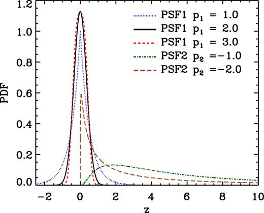
Distributions from which photo-z errors are drawn in Section 6.3. The parameter p1 controls the excess kurtoris of distributions from PDF1 and p2 the skewness and excess kurtosis of that from PDF2. All distributions from PDF1 are symmetric (zero skewness), where the ones with p1 = 2, p1 > 2, and p1 < 2 are Gaussians, boxier than Gaussians, and Gaussians with extended wings like Lorentzians, respectively. The distributions from PDF2 are positively skewed, and their skewness and excess kurtosis grow with p2.

Figure 10.

Distributions from which photo-z errors are drawn in Section 6.3. The parameter p₁ controls the excess kurtoris of distributions from PDF1 and p₂ the skewness and excess kurtosis of that from PDF2. All distributions from PDF1 are symmetric (zero skewness), where the ones with p₁ = 2, p₁ > 2, and p₁ < 2 are Gaussians, boxier than Gaussians, and Gaussians with extended wings like Lorentzians, respectively. The distributions from PDF2 are positively skewed, and their skewness and excess kurtosis grow with p₂.

Open in new tab Download slide

In Fig. 11 we present the value of α₀, α₂, and α₄ extracted from the BAO analysis of the average moments of 100 samples from the COLA ensemble after assuming a Gaussian PDF in the analysis. The number density of these samples is n = 10⁻²h³ Mpc⁻³, their photo-z errors are drawn from the distributions displayed in Fig. 10, and the difference between the 84th and 16th percentiles of those distributions is set to be |$\sigma_z=0.3\, \hbox{ per cent}$|⁠. The grey coloured regions indicate the 1 σ confidence region for a Gaussian PDF, and the error bars for the other distributions. For extreme PDFs, this could in principle introduce systematic errors in the estimation of α_ℓ. In practice we can see that even considering extreme PDFs and assuming a Gaussian PDF in the BAO analysis, the results are compatible to within 1σ. In addition, the shift in the stretch parameter is largely insensitive to the actual shape of the PDF.

Shift and uncertainty in α0, α2, and α4 from BAO analysis of 100 samples from the COLA ensemble with n = 10−2h3 Mpc−3 and photo-z errors drawn from different PDFs, where in the analysis we assume that they are drawn from a Gaussian PDF. The grey coloured areas enclose the 1 σ confidence region from the analysis of samples with Gaussian photo-z errors. The employed PDFs are shown in Fig. 10. Even for photo-z errors drawn from PDFs with large excess kurtosis and skewness, the results are compatible with the Gaussian case at the 1 σ level.

Figure 11.

Shift and uncertainty in α₀, α₂, and α₄ from BAO analysis of 100 samples from the COLA ensemble with n = 10⁻²h³ Mpc⁻³ and photo-z errors drawn from different PDFs, where in the analysis we assume that they are drawn from a Gaussian PDF. The grey coloured areas enclose the 1 σ confidence region from the analysis of samples with Gaussian photo-z errors. The employed PDFs are shown in Fig. 10. Even for photo-z errors drawn from PDFs with large excess kurtosis and skewness, the results are compatible with the Gaussian case at the 1 σ level.

Open in new tab Download slide

In this section we have disregarded the possibility of interlopers – objects systematically assigned to incorrect redshifts. This may happen to unobscured quasars and star-forming galaxies in medium- and narrow-band surveys, as pairs of emission lines at different redshifts may fall in the same filters, which is translated into a redshift PDF with two or more peaks (see e.g. fig. 4 of Chaves-Montero et al. 2017). If the percentage of interlopers is very small, at first order their net effect is to increase the shot noise level as they are uncorrelated with the main sample. They can be accounted for by artificially increasing the shot noise level. Nonetheless, if their amount is significant with respect to the main sample, they introduce anisotropies in the galaxy clustering (Lidz & Taylor 2016), where these anisotropies open the possibility of using AP-type tests (Alcock & Paczynski 1979) to correct for them.

We note that all expressions in this work are given for arbitrary PDFs. Therefore, if it is possible to know the PDF of photo-z errors, its actual shape can be used in BAO analyses.

6.4 Extracting cosmological information from BAO and impact of number density

As explained in Section 6.2, the constraining power of BAO depends on the scale at which the shot noise level starts dominating the amplitude of power spectrum moments. In this section we address how the precision in measuring cosmological parameters from BAO analyses (H and D_A) depends on the number density of the analysed sample. For this, we re-analyse our COLA samples randomly diluted to have |$\bar{n} = [10^{-2}, \, 3\times 10^{-3}, \,10^{-3}, \,3\times 10^{-4}, \,10^{-4}]\,h^3\mathrm{Mpc}^{-3}$|⁠.

In the top and bottom panels of Fig. 12 we present the average precision in measuring σ_⊥ and σ|$_{\parallel}$| from 1 000 COLA samples with n = 10⁻² and 10⁻³ h³ Mpc⁻³, respectively. Contours enclose the 1 σ confidence region for samples with different Gaussian photo-z errors, as stated in the legend. The uncertainty in σ|$_{\parallel}$| (after marginalizing over σ_⊥) always increases with the size of photo-z errors, which is because the error ellipses rotate anticlockwise as photo-z errors grow. Nevertheless, the uncertainty in σ_⊥ and the Figure-of-Merit (FoM) of this combination of parameters (the inverse of the ellipse’s area) do not monotonically grow with the size of photo-z errors. For the number densities studied here, we find that for |$\sigma_z=0.3\, \hbox{ per cent}$| the precision in measuring D_A is greater than for samples with σ_z = 0, which highlights that the analysis of power spectrum moments might not optimally extract the cosmological information encoded in BAO perpendicular to the LOS. We further explore this in the next section.

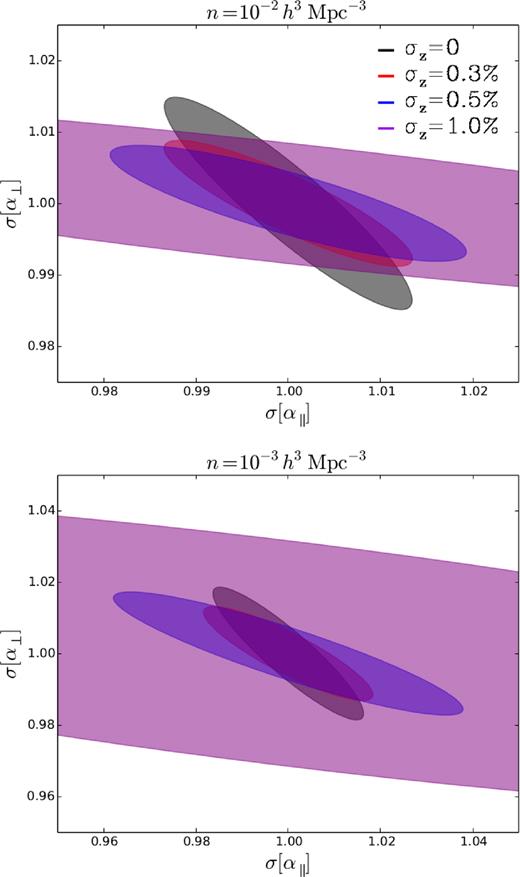
Uncertainty in the parallel and perpendicular components of the stretch parameter for samples with n = 10−2 and 10−3 h3 Mpc−3 (top and bottom panels, respectively), where they control the precision measuring H and DA, respectively. As we can see, the uncertainty in H after marginalizing over DA grows with the size of photo-z errors, as the error ellipses rotate in the anticlockwise direction. However, the FoM (inverse of the ellipse’s area) does not monotonically decrease with σz, which means that the combination of H and DA is not always measured with more precision by samples with no photo-z errors from the analysis of power spectrum moments.

Figure 12.

Uncertainty in the parallel and perpendicular components of the stretch parameter for samples with n = 10⁻² and 10⁻³ h³ Mpc⁻³ (top and bottom panels, respectively), where they control the precision measuring H and D_A, respectively. As we can see, the uncertainty in H after marginalizing over D_A grows with the size of photo-z errors, as the error ellipses rotate in the anticlockwise direction. However, the FoM (inverse of the ellipse’s area) does not monotonically decrease with σ_z, which means that the combination of H and D_A is not always measured with more precision by samples with no photo-z errors from the analysis of power spectrum moments.

Open in new tab Download slide

To continue exploring the constraints on cosmological parameters as a function of number density and photo-z errors, in the left-hand, middle, and right-hand panels of Fig. 13 we display the precision in H, D_A, and the FoM of both parameters, respectively. The uncertainty in each parameter is computed after marginalizing over the other. Symbols and lines indicate the results from simulations and the analytic model introduced in equation (33), respectively, where the free parameters of the model are fitted to reproduce the results from simulations. Their value is A₀ = 0.35, A₂ = 0.50, A₄ = 0.55, and c = 0.3. As expected, the uncertainty in H grows with the size of photo-z errors and by decreasing the number density. However, it is important to notice that the precision in H is the same for samples with |$\sigma_z=0.5\, \hbox{ per cent}$| and n = 10⁻³ h³ Mpc⁻³ and as for samples no photo-z errors and 10⁻⁴ h³ Mpc⁻³. As spectro-photometric surveys detect in general fainter objects than spectroscopic surveys, future wide-field surveys with dozens of photometric bands such as J-PAS will be competitive with spectroscopic surveys measuring cosmological parameters from BAO analyses.

$Precision measuring the Hubble parameter (left-hand panel), the angular diameter distance (middle panel), and their FoM from the BAO analysis of samples with different number densities and Gaussian photo-z errors. Each symbol indicates the average result from 1 000 samples from the COLA ensemble and the lines show analytic predictions from equation (33) using A0 = 0.35, A2 = 0.50, A4 = 0.55, and c = 0.3. The uncertainty in H grows with the size of photo-z errors and by decreasing the number density. On the other hand, the behaviour of σ[DA] is more complex, where samples with sub-percent photo-z errors have more precision measuring DA than samples with no errors. This highlights that all the cosmological information encoded on BAO is not recovered from the analysis of power spectrum moments. Black crosses indicate the results after deconvolving the effect of RSD using equation (46) in samples with 10−2 h3 Mpc−3 and no photo-z errors. This simple algorithm increases by $54\, \hbox{ per cent}$ the precision measuring DA.$

Figure 13.

Precision measuring the Hubble parameter (left-hand panel), the angular diameter distance (middle panel), and their FoM from the BAO analysis of samples with different number densities and Gaussian photo-z errors. Each symbol indicates the average result from 1 000 samples from the COLA ensemble and the lines show analytic predictions from equation (33) using A₀ = 0.35, A₂ = 0.50, A₄ = 0.55, and c = 0.3. The uncertainty in H grows with the size of photo-z errors and by decreasing the number density. On the other hand, the behaviour of σ[D_A] is more complex, where samples with sub-percent photo-z errors have more precision measuring D_A than samples with no errors. This highlights that all the cosmological information encoded on BAO is not recovered from the analysis of power spectrum moments. Black crosses indicate the results after deconvolving the effect of RSD using equation (46) in samples with 10⁻² h³ Mpc⁻³ and no photo-z errors. This simple algorithm increases by |$54\, \hbox{ per cent}$| the precision measuring D_A.

Open in new tab Download slide

The precision measuring D_A and the FoM of H and D_A shows a non-monotonic behaviour with σ_z for samples with a large number of densities, whereas at smaller number densities they are proportional to the size of photo-z errors. As we have commented above, we leave the discussion of this to the following section.

Our analytic model, which only employs the real-space l = 0 moment as input, reasonably fits the results from simulations. Therefore, it can be used to make forecasts for the precision measuring cosmological parameters from samples with different number densities, linear biases, photo-z errors, and cosmologies. Furthermore, we can use this model to look for the best sample to constrain cosmology. All the above considerations should be taken into account for the optimal design of future galaxy surveys. For instance, the photo-z errors for a given galaxy sample might depend not only on the hardware employed, but also on the intrinsic properties of galaxies (e.g. brighter objects having more accurate redshift estimates). In such a case, the sample that delivers the strongest constraints on cosmological parameters is not necessarily the one with the smallest photo-z errors.

6.5 Loss of transverse information from the analysis of power spectrum moments

As we showed in the previous section, for a large number of densities D_A is measured with more precision from samples with sub-percent photo-z errors than from samples with no errors. We obtain the same results from simulations and from the analytic model introduced in equation (33). As the introduction of photo-z errors cannot increase the amount of cosmological information, this highlights that the analysis of power spectrum moments does not extract all the cosmological information encoded in BAO. Therefore, it is worth to follow other approaches such as the analysis of the full anisotropic power spectrum (e.g. Ballinger, Peacock & Heavens 1996).

This reduction of the cosmological information available from BAO analyses only appears in redshift space. RSDs suppress more strongly parallel k-modes, and when we take the angular average of the power spectrum to compute its moments, we treat in the same way all k-modes, even when the ones parallel to the LOS are noisier. Consequently, the resulting power spectrum obtained after averaging over all k-modes in a k-bin is noisier than if only perpendicular k-modes are considered. For samples with photo-z errors this is not the case, as they reduce the weight of parallel k-modes during the angular average, and thus the uncertainty after angular averaging over all k-modes is approximately the same as for perpendicular k modes (cf. Section 4.1).

To probe that the angular average of k-modes with different uncertainties causes D_A to be measured with smaller precision, we deconvolve the effect of RSD from power spectrum moments:

\begin{eqnarray*} \tilde{P}(k)= \left\langle \frac{n\hat{P}(k, \mu )-1}{n{\cal F}^2(k, \mu )} \right\rangle_{\hat{\boldsymbol{k}}}. \end{eqnarray*}

(46)

In Fig. 14 we show the average uncertainty in cosmological parameters computed from 1 000 samples of the COLA ensemble with n = 10⁻² h³ Mpc⁻³ and no photo-z errors. The purple, grey, and blue ellipses indicate the results in real space, redshift space, and redshift space after deconvolving the effect of RSD. Our deconvolution procedure increases the precision measuring D_A and the FoM of H and D_A by |$54\, \hbox{ per cent}$| and |$37\, \hbox{ per cent}$|⁠, respectively, and, as expected, it does not reduce σ[H]. Nevertheless, our naive approach does not totally correct the effect of RSD, as real-space power spectrum moments measure H and D_A with greater precision.

$Same as Fig. 12 for samples with n = 10−2 h3 Mpc−3 and no photo-z errors in real space, redshift space, and redshift space after deconvolving the effect of RSD (in purple, grey, and blue, respectively). The strongest constraints on H (σ[α$_{\parallel}$]) come from real-space moments because RSD further suppress BAO along the LOS. The constraints on DA (σ[α⊥]) should be approximately the same in real- and redshift-space; however, the precision measuring DA is 2.4 times smaller in redshift space. As we can see, this is partially corrected by the deconvolution procedure introduced in Section 6.5.$

Figure 14.

Same as Fig. 12 for samples with n = 10⁻² h³ Mpc⁻³ and no photo-z errors in real space, redshift space, and redshift space after deconvolving the effect of RSD (in purple, grey, and blue, respectively). The strongest constraints on H (σ[α|$_{\parallel}$|]) come from real-space moments because RSD further suppress BAO along the LOS. The constraints on D_A (σ[α_⊥]) should be approximately the same in real- and redshift-space; however, the precision measuring D_A is 2.4 times smaller in redshift space. As we can see, this is partially corrected by the deconvolution procedure introduced in Section 6.5.

Open in new tab Download slide

We note that equation (46) cannot be applied to samples with photo-z errors on intermediate and small scales. This is because they strongly suppress k-modes with μ ≃ 1, which causes them to be completely dominated by shot noise, and our shot noise subtraction is not accurate enough in this regime. Nonetheless, a correct characterization of shot noise in this regime could lead to a joint deconvolution of RSD and photo-z errors. We note that there are other approaches in the literature to reduce the impact of photo-z errors on the power spectrum (e.g. McQuinn & White 2013).

7 FORECASTS FOR FUTURE GALAXY SURVEYS

In Section 4.3 we introduced an analytic expression to compute the precision measuring cosmological parameters from BAO analyses, and in the previous section we showed that this model approximately reproduces the results from numerical simulations. In this section we use this expression to forecast the precision in H from future spectro-photometric surveys at z = 1. We note that the results of this section are illustrative.

In what follows, we will assume that the number density of galaxies linearly scale with the size of photo-z errors (see table 8 of Benitez et al. 2014) and that the analysed volume is |$v$| = 78.7 Gpc³, i.e. the same volume as each COLA simulation. In particular, we take the relation between number density and photo-z errors to be n = 5(1 + 10³σ_z)10⁻⁴ h³ Mpc⁻³. In Fig. 15 we display the precision measuring H after marginalizing over D_A from galaxy samples with b = 2 and different photo-z errors. For samples with |$\sigma_z\le 0.3\, \hbox{ per cent}$|⁠, the precision measuring H is approximately the same. On the other hand, for |$\sigma_z\,\,{>}\,\,0.3\, \hbox{ per cent}$| the uncertainty in H is rapidly increased. This encourages the employment of spectroscopic and spectro-photometric surveys with |$\sigma_z\,\,{<}\,\,0.5\, \hbox{ per cent}$| to study the expansion history of the Universe.

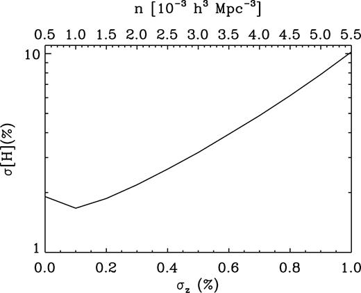
$Forecasts for the precision measuring H in spectro-photometric galaxy surveys at z = 1. The results are computed assuming a comoving volume of $v$ = 78.7 Gpc3 and that the number density of galaxies linearly scales with σz. As we can see, galaxy samples with $\sigma_z\le 0.3\, \hbox{ per cent}$ measure the Hubble parameter with approximately the same precision.$

Figure 15.

Forecasts for the precision measuring H in spectro-photometric galaxy surveys at z = 1. The results are computed assuming a comoving volume of |$v$| = 78.7 Gpc³ and that the number density of galaxies linearly scales with σ_z. As we can see, galaxy samples with |$\sigma_z\le 0.3\, \hbox{ per cent}$| measure the Hubble parameter with approximately the same precision.

Open in new tab Download slide

In summary, to design and fully exploit galaxy surveys that employ noisy estimators to compute redshifts, it is necessary to carefully select the properties of the target galaxy sample.

8 CONCLUSIONS

The next generation of galaxy surveys will dramatically increase the precision of measurements for the expansion and growth history of the Universe. Some of these surveys will observe large areas of the sky with linear variable filters or dozens of narrow-bands, providing a low-resolution spectra for every region of the sky. In addition, they will measure the redshift of millions of galaxies with sub-percent accuracy, offering a promising way of constraining cosmological parameters. Nevertheless, to fully exploit this new kind of data, it is necessary to fully characterize the effect of photo-z errors on cosmological observables.

In this work we presented a detailed study of the impact of sub-percent photo-z errors on the clustering of galaxies in Fourier space, with an emphasis on the BAO signal. We derived analytic expressions for how photo-z errors modify power spectrum moments, their variances, and the smearing of BAO, which we compared with the results from 1 000 N-body simulations.

Our main findings can be summarized as follows:

In real space photo-z errors suppress power spectrum moments on intermediate and small scales. This increases the interval of scales dominated by shot noise, which reduces the range of scales available for BAO analyses. There is an additional effect in redshift space: the suppression of angular-averaged BAO wiggles gets weaker with increasing photo-z errors. This is because photo-z errors reduce the weight of LOS k-modes in computing power spectrum moments which have more diluted BAO signal due to non-linear RSD.
We derived how the cosmological information encoded in BAO depends on the properties of the galaxy sample studied. We showed that small-scale RSD and/or photo-z errors induce a scale dependence on this information, where the dependence on the Hubble parameter (angular diameter distance) decreases (increases) with the size of photo-z errors.
Based on these findings, we built a model for extracting cosmological information from the analysis of power spectrum moments. Then, we applied it to simulated galaxy catalogues with different number densities and photo-z errors. We found that photo-z errors do not introduce an additional shift in the position of the BAO scale with respect to the no photo-z error case. Therefore, they do not bias the cosmological information encoded in BAOs. In addition, we found that assuming that photo-z errors are Gaussian in BAO analyses, even when they are drawn from PDFs with large excess kurtosis and skewness, does not bias the results.
In Section 6.4 we analysed the precision measuring the Hubble parameter and the angular diameter distance from samples with different number densities and photo-z errors. We found that for the same number density, the uncertainty in measuring H decreases with the size of photo-z errors. Nevertheless, it is still possible to measure H with the same (or more) precision from samples with sub-percent photo-z errors as from samples with no errors if the number density of the first is increased. Finally, we also found that the analysis of power spectrum moments artificially decreases the precision in measuring D_A. We suggest to analyse the 2D power spectrum in future studies.

Our results encourage the measurement of cosmological parameters from spectro-photometric surveys, as in general they are deeper than spectroscopic surveys for the same integration time. In Section 7 we forecast the precision in measuring the Hubble parameter from BAO analyses assuming that the number density of galaxies linearly scales with the size photo-z errors. Roughly, we found the same results for galaxy samples with redshift uncertainties smaller than |$\sigma_z=0.4\, \hbox{ per cent}$|⁠. This means that galaxy surveys with sub-percent photo-z errors could set constraints on the dark energy equation of state as precise as spectroscopic surveys.

Along this paper we put a focus on extracting cosmological information from galaxy samples with sub-percent photo-z errors. Recently, Ross et al. (2017) conducted a similar investigation in configuration space for samples with photo-z errors of a few per cent, finding that for those the BAO feature mostly constrains D_A(z) and that the projected correlation function is enough for extracting all cosmological information. Their findings agree with ours for samples with |$\sigma_z = 1\, \hbox{ per cent}$|⁠, as we can see in Figs 12 and 13. Nevertheless, as we show along this work, for samples with smaller photo-z errors H(z) can be constrained from the 3D galaxy clustering.

Finally, our paper highlights that photo-z errors substantially increase the complexity of the extraction of cosmological information from BAO analyses. Therefore, it is crucial a thorough understanding and modelling of photo-z errors in galaxy clustering. We hope our work to have clarified some the most important aspects of this issue, and that it will help in the cosmological analysis of future spectro-photometric surveys.

Footnotes

1

In what follows we will assume that |$\alpha_\parallel^2/\alpha_\perp^2=1$| and thus ε = 1.

2

We note that this procedure has never been applied to reconstruct the 3D density field of galaxy samples with photo-z errors.

ACKNOWLEDGEMENTS

We thank the anonymous referee for the thorough review, insightful comments, and positive suggestions. We acknowledge discussions with Raul Abramo, Andreu Font-Ribera, Licia Verde, and Carlos López-Sanjuan. Argonne National Laboratory’s work was supported by the U.S. Department of Energy, Office of Science, Office of Nuclear Physics, under contract DE-AC02-06CH11357. The authors acknowledge support from the Spanish Ministry of Economy and Competitiveness (MINECO) through the project AYA2015-66211-C2-2. JCM acknowledges support from the Fundación Bancaria Ibercaja for developing this research. REA acknowledges support from the European Research Council through grant number ERC-StG/716151. CHM acknowledges support from the Ramon y Cajal Fellow Program of the Spanish MINECO. This project has received funding from the European Union’s Horizon 2020 Research and Innovation Programme under the Marie Sklodowska-Curie grant agreement No. 734374.

REFERENCES

Abramowitz

M.

,

Stegun

I. A.

,

1972

,

Handbook of Mathematical Functions

,

United States Department of Commerce, National Institute of Standards and Technology

,

New York: Dover

Google Scholar

Google Preview

OpenURL Placeholder Text

WorldCat

Alcock

C.

,

Paczynski

B.

,

1979

,

Nature

,

281

,

358

10.1038/281358a0

Crossref

Search ADS

Angulo

R. E.

,

Pontzen

A.

,

2016

,

MNRAS

,

462

,

L1

10.1093/mnrasl/slw098

Crossref

Search ADS

Angulo

R. E.

,

Baugh

C. M.

,

Frenk

C. S.

,

Lacey

C. G.

,

2008

,

MNRAS

,

383

,

755

10.1111/j.1365-2966.2007.12587.x

Crossref

Search ADS

Angulo

R. E.

,

Springel

V.

,

White

S. D. M.

,

Jenkins

A.

,

Baugh

C. M.

,

Frenk

C. S.

,

2012

,

MNRAS

,

426

,

2046

10.1111/j.1365-2966.2012.21830.x

Crossref

Search ADS

Angulo

R. E.

,

White

S. D. M.

,

Springel

V.

,

Henriques

B.

,

2014

,

MNRAS

,

442

,

2131

10.1093/mnras/stu905

Crossref

Search ADS

Ballinger

W. E.

,

Peacock

J. A.

,

Heavens

A. F.

,

1996

,

MNRAS

,

282

,

877

10.1093/mnras/282.3.877

Crossref

Search ADS

Benítez

N.

et al. ,

2009

,

ApJ

,

691

,

241

10.1088/0004-637X/691/1/241

Crossref

Search ADS

Benitez

N.

et al. ,

2014

, arXiv:e-prints

Bjerhammar

A.

,

1951

,

Trans. Roy. Inst. Tech. Stockholm

,

1951

,

86

pp.

(2 plates)

Blake

C.

,

Bridle

S.

,

2005

,

MNRAS

,

363

,

1329

10.1111/j.1365-2966.2005.09526.x

Crossref

Search ADS

Cai

Y.-C.

,

Angulo

R. E.

,

Baugh

C. M.

,

Cole

S.

,

Frenk

C. S.

,

Jenkins

A.

,

2009

,

MNRAS

,

395

,

1185

10.1111/j.1365-2966.2009.14402.x

Crossref

Search ADS

Chaves-Montero

J.

et al. ,

2017

,

MNRAS

,

472

,

2085

10.1093/mnras/stx2054

Crossref

Search ADS

Colombi

S.

,

Jaffe

A.

,

Novikov

D.

,

Pichon

C.

,

2009

,

MNRAS

,

393

,

511

10.1111/j.1365-2966.2008.14176.x

Crossref

Search ADS

Crocce

M.

,

Scoccimarro

R.

,

2008

,

Phys. Rev. D

,

77

,

023533

10.1103/PhysRevD.77.023533

Crossref

Search ADS

Dalton

G.

et al. ,

2014

, in

Proc. SPIE Conf. Ser., Vol. 9147

,

Ground-Based and Airborne Instrumentation for Astronomy V. SPIE

,

Bellingham

, p.

91470L

de Jong

R.

,

2011

,

The Messenger

,

145

,

14

DESI Collaboration

et al. ,

2016

,

arXiv:e-prints

Dolney

D.

,

Jain

B.

,

Takada

M.

,

2006

,

MNRAS

,

366

,

884

10.1111/j.1365-2966.2005.09606.x

Crossref

Search ADS

Doré

O.

et al. ,

2014

,

arXiv:e-prints

Doré

O.

et al. ,

2016

,

arXiv:e-prints

Eisenstein

D. J.

,

Hu

W.

,

1998

,

ApJ

,

496

,

605

10.1086/305424

Crossref

Search ADS

Eisenstein

D. J.

et al. ,

2005

,

ApJ

,

633

,

560

10.1086/466512

Crossref

Search ADS

Eisenstein

D. J.

,

Seo

H.-J.

,

Sirko

E.

,

Spergel

D. N.

,

2007

,

ApJ

,

664

,

675

10.1086/518712

Crossref

Search ADS

Foreman-Mackey

D.

,

Hogg

D. W.

,

Lang

D.

,

Goodman

J.

,

2013

,

PASP

,

125

,

306

10.1086/670067

Crossref

Search ADS

Glazebrook

K.

,

Blake

C.

,

2005

,

ApJ

,

631

,

1

10.1086/432497

Crossref

Search ADS

Hartlap

J.

,

Simon

P.

,

Schneider

P.

,

2007

,

A&A

,

464

,

399

Crossref

Search ADS

Hockney

R. W.

,

Eastwood

J. W.

,

1981

,

Computer Simulation Using Particles

,

McGraw-Hill

,

New York

Google Scholar

Google Preview

OpenURL Placeholder Text

WorldCat

Howlett

C.

,

Manera

M.

,

Percival

W. J.

,

2015

,

Astron. Comput.

,

12

,

109

10.1016/j.ascom.2015.07.003

Crossref

Search ADS

Ilbert

O.

et al. ,

2009

,

ApJ

,

690

,

1236

10.1088/0004-637X/690/2/1236

Crossref

Search ADS

Kaiser

N.

,

1987

,

MNRAS

,

227

,

1

10.1093/mnras/227.1.1

Crossref

Search ADS

Kashlinsky

A.

,

Hernández-Monteagudo

C.

,

Atrio-Barandela

F.

,

2001

,

ApJ

,

557

,

L1

10.1086/323172

Crossref

Search ADS

Koda

J.

,

Blake

C.

,

Beutler

F.

,

Kazin

E.

,

Marin

F.

,

2016

,

MNRAS

,

459

,

2118

10.1093/mnras/stw763

Crossref

Search ADS

Laureijs

R.

et al. ,

2011

,

arXiv:e-prints

Lidz

A.

,

Taylor

J.

,

2016

,

ApJ

,

825

,

143

10.3847/0004-637X/825/2/143

Crossref

Search ADS

Martí

P.

,

Miquel

R.

,

Castander

F. J.

,

Gaztañaga

E.

,

Eriksen

M.

,

Sánchez

C.

,

2014

,

MNRAS

,

442

,

92

10.1093/mnras/stu801

Crossref

Search ADS

McQuinn

M.

,

White

M.

,

2013

,

MNRAS

,

433

,

2857

10.1093/mnras/stt914

Crossref

Search ADS

Moore

R. L.

,

1920

,

Bull. Am. Math. Soc.

,

26

,

412

10.1090/S0002-9904-1920-03332-X

Crossref

Search ADS

Orsi

A. A.

,

Angulo

R. E.

,

2018

,

MNRAS

,

475

,

2530

,

Padmanabhan

N.

,

White

M.

,

2008

,

Phys. Rev. D

,

77

,

123540

10.1103/PhysRevD.77.123540

Crossref

Search ADS

Padmanabhan

N.

,

White

M.

,

2009

,

Phys. Rev. D

,

80

,

063508

10.1103/PhysRevD.80.063508

Crossref

Search ADS

Peacock

J. A.

,

Dodds

S. J.

,

1994

,

MNRAS

,

267

,

1020

10.1093/mnras/267.4.1020

Crossref

Search ADS

Penrose

R.

,

1955

,

Proc. Cambridge Philos. Soc.

,

51

,

406

10.1017/S0305004100030401

Crossref

Search ADS

Ross

A. J.

,

Percival

W. J.

,

Manera

M.

,

2015

,

MNRAS

,

451

,

1331

10.1093/mnras/stv966

Crossref

Search ADS

Ross

A. J.

, et al. ,

2017

,

MNRAS

,

472

,

4456

Sánchez

A. G.

,

Baugh

C. M.

,

Angulo

R. E.

,

2008

,

MNRAS

,

390

,

1470

Schmittfull

M.

,

Feng

Y.

,

Beutler

F.

,

Sherwin

B.

,

Chu

M. Y.

,

2015

,

Phys. Rev. D

,

92

,

123522

10.1103/PhysRevD.92.123522

Crossref

Search ADS

Scoccimarro

R.

,

2004

,

Phys. Rev. D

,

70

,

083007

10.1103/PhysRevD.70.083007

Crossref

Search ADS

Sefusatti

E.

,

Crocce

M.

,

Scoccimarro

R.

,

Couchman

H. M. P.

,

2016

,

MNRAS

,

460

,

3624

10.1093/mnras/stw1229

Crossref

Search ADS

Seo

H.-J.

,

Eisenstein

D. J.

,

2003

,

ApJ

,

598

,

720

10.1086/379122

Crossref

Search ADS

Seo

H.-J.

,

Eisenstein

D. J.

,

2007

,

ApJ

,

665

,

14

10.1086/519549

Crossref

Search ADS

Sereno

M.

,

Veropalumbo

A.

,

Marulli

F.

,

Covone

G.

,

Moscardini

L.

,

Cimatti

A.

,

2015

,

MNRAS

,

449

,

4147

10.1093/mnras/stv280

Crossref

Search ADS

Smith

R. E.

,

Scoccimarro

R.

,

Sheth

R. K.

,

2008

,

Phys. Rev. D

,

77

,

043525

10.1103/PhysRevD.77.043525

Crossref

Search ADS

Szapudi

I.

,

Prunet

S.

,

Pogosyan

D.

,

Szalay

A. S.

,

Bond

J. R.

,

2001

,

ApJ

,

548

,

L115

10.1086/319105

Crossref

Search ADS

Tassev

S.

,

Zaldarriaga

M.

,

Eisenstein

D. J.

,

2013

,

J. Cosmol. Astropart. Phys.

,

6

,

036

10.1088/1475-7516/2013/06/036

Crossref

Search ADS

Weinberg

D. H.

,

Mortonson

M. J.

,

Eisenstein

D. J.

,

Hirata

C.

,

Riess

A. G.

,

Rozo

E.

,

2013

,

Phys. Rep.

,

530

,

87

10.1016/j.physrep.2013.05.001

Crossref

Search ADS

Xu

X.

,

Cuesta

A. J.

,

Padmanabhan

N.

,

Eisenstein

D. J.

,

McBride

C. K.

,

2013

,

MNRAS

,

431

,

2834

10.1093/mnras/stt379

Crossref

Search ADS

Published by Oxford University Press on behalf of The Royal Astronomical Society 2018.

This work is written by (a) US Government employee(s) and is in the public domain in the US.

Download all slides

Month:	Total Views:
April 2018	43
May 2018	27
June 2018	30
July 2018	25
August 2018	20
September 2018	20
October 2018	7
November 2018	14
December 2018	18
January 2019	9
February 2019	16
March 2019	15
April 2019	28
May 2019	13
June 2019	7
July 2019	5
August 2019	8
September 2019	9
October 2019	24
November 2019	9
December 2019	8
January 2020	13
February 2020	13
March 2020	7
April 2020	7
May 2020	8
June 2020	12
July 2020	18
August 2020	6
September 2020	5
October 2020	6
November 2020	7
December 2020	4
January 2021	8
February 2021	18
March 2021	11
April 2021	8
May 2021	7
June 2021	3
July 2021	14
August 2021	9
September 2021	5
October 2021	12
November 2021	9
December 2021	17
January 2022	7
February 2022	5
March 2022	5
April 2022	11
May 2022	6
June 2022	8
July 2022	10
August 2022	11
September 2022	15
October 2022	6
November 2022	6
December 2022	6
January 2023	12
February 2023	3
March 2023	20
April 2023	8
May 2023	3
June 2023	8
July 2023	2
August 2023	4
September 2023	7
October 2023	4
November 2023	8
December 2023	16
January 2024	8
February 2024	4
March 2024	29
April 2024	16
May 2024	8
June 2024	10
July 2024	24
August 2024	6
September 2024	8
October 2024	10
November 2024	15
December 2024	7
January 2025	12
February 2025	4
March 2025	14
April 2025	1
May 2025	5

Article Contents

The effect of photometric redshift uncertainties on galaxy clustering and baryonic acoustic oscillations Free

Abstract

1 INTRODUCTION

2 NUMERICAL METHODS

2.1 Numerical simulations

2.2 Power spectrum and covariance measurements

2.3 Redshift uncertainties

3 EFFECT OF PHOTOMETRIC REDSHIFT ERRORS ON POWER SPECTRUM MOMENTS

3.1 Power spectrum moments

3.1.1 General expressions

3.1.2 The Gaussian case

3.1.3 Comparison with numerical simulations

3.2 Variance of power spectrum moments

3.2.1 General expressions

3.2.2 Comparison with simulations: diagonal terms

3.2.3 Comparison with simulations: off-diagonal terms

3.3 Signal-to-noise ratio

3.3.1 Toy model

3.3.2 Comparison with simulations

4 EFFECT OF PHOTOMETRIC REDSHIFT ERRORS ON BAO

4.1 The shape of the BAO signal

4.1.1 The Gaussian case and comparison with simulations

4.2 Cosmological information encoded in BAO

4.3 Toy model for the uncertainty in the stretch parameter

4.4 The scale dependence of cosmological information

5 EXTRACTING INFORMATION FROM BAO

5.1 Modelling power spectrum moments

5.2 Parameter likelihood calculation

6 RESULTS FROM SIMULATED CATALOGUES

6.1 Quality of our model

6.2 Effect of redshift errors

6.3 Effect of different PDFs for photometric redshift errors

6.4 Extracting cosmological information from BAO and impact of number density

6.5 Loss of transverse information from the analysis of power spectrum moments

7 FORECASTS FOR FUTURE GALAXY SURVEYS

8 CONCLUSIONS

Footnotes

ACKNOWLEDGEMENTS

REFERENCES

Citations

Views

Altmetric

Email alerts

Astrophysics Data System

Citing articles via

Latest

Most Read

Most Cited

This Feature Is Available To Subscribers Only

The effect of photometric redshift uncertainties on galaxy clustering and baryonic acoustic oscillations