


Abstract
Massive black hole binaries (MBHBs) are expected to form at the centre of merging galaxies during the hierarchical assembly of the cosmic structure, and are expected to be the loudest sources of gravitational waves (GWs) in the low-frequency domain. However, because of the dearth of energy exchanges with background stars and gas, many of these MBHBs may stall at separations that are too large for GW emission to drive them to coalescence in less than a Hubble time. Triple MBH systems are then bound to form after a further galaxy merger, triggering a complex and rich dynamics that can eventually lead to MBH coalescence. Here, we report on the results of a large set of numerical simulations, where MBH triplets are set in spherical stellar potentials and MBH dynamics is followed through 2.5 post-Newtonian orders in the equations of motion. From our full suite of simulated systems, we find that a fraction ( ≃ 20–30 per cent) of the MBH binaries that would otherwise stall is led to coalesce within a Hubble time. The corresponding coalescence time-scale peaks around 300 Myr, while the eccentricity close to the plunge, albeit small, is non-negligible (≲0.1). We construct and discuss marginalized probability distributions of the main parameters involved and, in a companion paper of the series, we will use the results presented here to forecast the contribution of MBH triplets to the GW signal in the nHz regime probed by Pulsar Timing Array experiments.
1 INTRODUCTION
Massive black holes (MBHs) are ubiquitous in the nuclei of nearby spheroids (see Kormendy & Ho 2013, and references therein), and are recognized to be a fundamental ingredient in the process of galaxy formation and evolution. Indeed, the tight correlations existing among the mass of the central MBH and the properties of the host galaxy (see e.g. Ferrarese & Merritt 2000; Gebhardt et al. 2000; Tremaine et al. 2002; Ferrarese 2004; Ferrarese et al. 2006) indicate that galaxies and MBHs follow a linked evolutionary path during the formation history of cosmic structures. It is therefore understood that MBHs were commonly residing at the centres of galaxies at all cosmic epochs. This very circumstance, when framed in the bottom-up hierarchical clustering of cold dark matter overdensities, leads to the inevitable conclusion that a large number of MBH binaries (MBHBs) formed during the build-up of the large-scale structure (Begelman, Blandford & Rees 1980).
MBHBs are expected to be the loudest sources of gravitational radiation in the nHz–mHz frequency range (Haehnelt 1994; Jaffe & Backer 2003; Wyithe & Loeb 2003; Enoki et al. 2004; Sesana et al. 2004, 2005; Jenet et al. 2005; Rhook & Wyithe 2005; Barausse 2012; Klein et al. 2016), a regime partially covered by the Laser Interferometer Space Antenna (LISA) interferometer (Consortium et al. 2013; Amaro-Seoane et al. 2017) and by existing Pulsar Timing Array (PTA) experiments (The NANOGrav Collaboration 2015; Desvignes et al. 2016; Reardon et al. 2016; Verbiest et al. 2016). The observability of MBHBs by LISA and PTAs relies on the ability of the two black holes to coalesce within a Hubble time after a galaxy merger.1
The evolution of an MBHB in a galactic potential can be divided into three different stages (Begelman et al. 1980). Initially, driven by dynamical friction against stars and gas, the two MBHs migrate towards the centre of the newly formed spheroid to form a bound binary system. The subsequent evolution of the binary depends on the properties of the surrounding environment in the nucleus of the merger galaxy remnant. In gas-rich galaxies (wet mergers), further shrinking can be caused by the interaction with a massive circumbinary disc or with incoherent pockets of accreted gas clouds (Dotti et al. 2007; Cuadra et al. 2009; Nixon et al. 2011; Goicovic et al. 2017). However, most of the simulations exploring these scenarios are highly idealized, usually lacking realistic prescriptions for cooling, fragmentation, star formation, and supernova feedback. The actual efficiency of gas–MBHB interaction in realistic physical conditions is poorly known, and stalling of the binary is still a possibility (see e.g. Lodato et al. 2009). In dry galaxy mergers (i.e. where gas is absent/negligible and therefore cannot substantially affect the dynamics), an MBHB can evolve only because of stellar interactions. Indeed, after the MBHs form a bound pair at ai ≈ GM/σ2 (M = m1 + m2 is the total mass of the binary and σ is the stellar velocity dispersion), the binary hardens by ejecting stars via single three-body interactions. The efficiency of this process saturates at the hardening radius ah ∼ Gm2/4σ2 (where m2 is the mass of the secondary, Quinlan 1996) and beyond that point, the MBHB hardens at a constant rate. However, since in the process stars are ejected by the slingshot mechanism, the orbital decay soon falters, unless new stars are forced to replenish the otherwise depleting loss cone. Because typically ah ∼ 1 pc for ∼108 M⊙ black holes, it is not guaranteed that the MBHB can eventually close the gap down to separations agr ∼ 10−2 pc, i.e. the separations at which gravitational wave (GW) emission alone can drive the two MBHs to coalesce within a Hubble time. In the literature, this is often referred to as the ‘final parsec problem’ (Milosavljević & Merritt 2003).
In dry galaxy mergers, a possible important mechanism that could solve this problem is provided by triple MBH interactions. Triple systems can form when an MBHB stalled at separations ≲ah (because of the lack of sufficient gas and inefficient loss cone replenishment) interacts with a third MBH – the ‘intruder’ – carried by a new galaxy merger (see e.g. Mikkola & Valtonen 1990; Heinämäki 2001; Blaes, Lee & Socrates 2002; Hoffman & Loeb 2007; Kulkarni & Loeb 2012). More specifically, these hierarchical triplets – i.e. triple systems where the hierarchy of orbital separations defines an inner and an outer binary, the latter consisting of the intruder and the centre of mass of the former – may undergo Kozai–Lidov (K–L) oscillations (Kozai 1962; Lidov 1962). These resonances arise in the framework of a secular analysis of hierarchical triplets by Taylor-expanding the Hamiltonian of the system in powers of the inner-to-outer semimajor axis ratio, which is assumed to be small. The results of Kozai and Lidov, valid at the quadrupole order of approximation, demonstrate that if the intruder is on a highly inclined orbit with respect to the inner binary, the K–L mechanism tends to secularly increase the eccentricity of the inner binary, eventually driving it to coalescence. By considering a higher order approximation (octupole), richer physics arises, and in particular, significant eccentricity can build up even for triplets with low relative inclinations (see e.g. Naoz 2016, for a comprehensive review and references).
We have recently started a comprehensive study of post-Newtonian (PN) dynamics of MBH triplets in a cosmological framework, ultimately aiming at the full characterization of the GW signal from the cosmic population of MBHBs. In the first step of the project (Bonetti et al. 2016, hereafter Paper I), we have discussed the importance of both chaotic three-body encounters and the K–L mechanism in the dynamics of triplets, and we have presented and tested our three-body PN code, which includes a realistic galactic potential, orbital hardening of the outer binary, the effect of the dynamical friction on the early stages of the intruder dynamics, as well as the PN contributions to the dynamics (through 2PN order in the conservative sector and leading order in the dissipative one). As detailed in Paper I, the employed equations of motion are consistently derived from the three-body PN Hamiltonian, which, for the first time in the framework of the MBH interactions, allows us to take into account the effect of the PN three-body terms in the dynamics. Indeed, in the common practice, these kind of terms are usually not accounted for, as the two-body PN corrections are simply applied to each pair of bodies (see e.g. Mikkola & Merritt 2008; Rantala et al. 2017; Ryu et al. 2017). Finally, in a spin-off effort (Bonetti et al. 2017a), we have highlighted and solved some subtle problems affecting naive implementations of quadrupolar and octupolar gravitational waveforms from numerically integrated trajectories of three-body systems.
In this paper, formally the second of the series, we will perform a systematic study of the dynamics and evolution of MBH triplets. Employing the code presented in Paper I, we will explore a large region of the six-dimensional parameter space of these systems, in terms of MBH masses, eccentricities, and relative inclinations. This will allow us to fully characterize the evolution of MBH triplets in galactic potentials. In a companion paper (Bonetti et al. 2017b), we will then frame the whole picture in the hierarchical build-up of cosmic structures (Barausse 2012), adopting a semi-analytic model of galaxy and MBH co-evolution, and assess the contribution of MBH triplets to the stochastic background of nHz GWs. In a follow-up paper (Bonetti et al., in preparation), we will also explore the implications for the GW signal from MBHBs in the mHz regime targeted by LISA.
The paper is organized as follows: in Section 2 we describe the computational set-up used to perform the simulations; in Section 3 we present the results of our analysis, while in Section 4 we discuss in more detail the strengths and caveats of our work. Finally, in the last section, we draw our conclusions. Throughout the paper G and c represent Newton’s gravitational constant and the speed of light, respectively.
2 METHODOLOGY
We numerically integrate the orbits of MBH triplets formed by a stalled MBHB at the centre of a stellar spherical potential (m1, m2) and by a third MBH (m3) approaching the system from larger distances.
2.1 Galactic potential and scaling relations
The properties of the stellar distribution are detailed in Paper I (to which we refer for more details). Here, we only provide a brief summary of the adopted set-up.
We do not consider any dark matter (DM) extended component associated to the stellar background. The properties of the stellar background are kept fixed during the evolution of the MBH triplet, so that its properties are solely determined by the mass of the stalled MBHB through the scaling relations discussed above.
2.2 Initial orbital parameters
In principle, the complete characterization of a system of three MBHs requires specifying 21 parameters. However, the initial configuration of the considered systems allows us to reduce the number of free parameters.
We first fix the motion of the centre of mass (position and velocity), thus reducing the effective number of initial parameters to 15. We then note that the initial values of some orbital elements (see Fig. 1) do not play any major role in the dynamics. More specifically, among these we have the two arguments of pericentre, the two longitudes of the ascending node, and the two orbital phases. Indeed, the various physical processes (e.g. dynamical friction, stellar hardening, the precession due to the galactic potential, and the relativistic one), driving the evolution of MBHBs, quickly make these parameters ‘lose memory’ of their initial values, as soon as the three MBHs first bind in a hierarchical triplet. The number of considered initial parameters is then reduced to nine. Moreover, we set the initial semimajor axis of the m3 orbit to the scale radius r0 of the stellar bulge, which ultimately depends only on m1 + m2, thus reducing the number of relevant free parameters to eight. We have verified that our results are robust against this choice of initial semimajor axis.
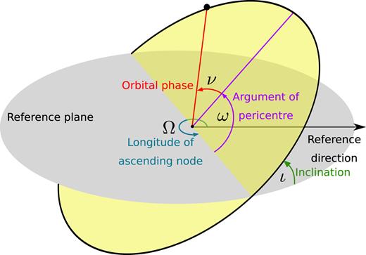
Schematic representation of a binary orbit in 3D space.
We note that the choice to initialize the inner binary as stalled implicitly determines its separation. In fact, according to a vast literature on the evolution of MBHBs (see e.g. Saslaw, Valtonen & Aarseth 1974; Begelman et al. 1980; Quinlan 1996; Yu 2002; Sesana, Haardt & Madau 2006) and the final parsec problem (Milosavljević & Merritt 2003; Vasiliev 2014; Vasiliev, Antonini & Merritt 2015), the binary shrinks to a separation ain ≲ ah, where ah ∼ Gm2/4σ2 represents the hardening radius of the stellar distribution. Further hardening of the system then proceeds at a nearly constant rate, dictated by the efficiency at which stars can be supplied to the binary loss cone. Depending on the properties of the host galaxy, evolution time-scales can be as long as several Gyr (see e.g. Yu 2002; Berczik et al. 2006; Khan, Just & Merritt 2011; Preto et al. 2011; Gualandris & Merritt 2012; Vasiliev 2014; Vasiliev, Antonini & Merritt 2014; Sesana & Khan 2015; Vasiliev et al. 2015; Khan et al. 2016; Gualandris et al. 2017). Therefore, we initialize the inner binary at a separation around ah, whose value, once m1 and m2 are specified, is completely determined. The exact value of ain is practically irrelevant as long as it is close to ah and sufficiently larger than agw, where agw represents the scale at which GW emission starts dominating the evolution of the binary. Specifically, for the initialization of ain ≲ ah, we assume (somewhat arbitrarily) ain/agw = (ah/agw)3/4, and we have checked that the results are robust against this choice. At this point, we are left with only seven free initial conditions.
Finally, the isotropy of the problem allows us to specify the relative inclination between the orbital planes of the two orbits, i.e. ι≡ ιin+ ιout, thus reducing the final set of relevant initial free parameters to six. We will explore this parameter space in the following.
In generating the initial conditions, for the mass of the heavier MBH of the inner binary (m1), we choose six values uniformly selected in logarithmic space, from 105 to 1010 M⊙. The inner and outer binary mass ratios qin ≡ m2/m1 and qout ≡ m3/(m1 + m2) can take four values each, uniformly spaced (logarithmically) from 0.03 to 1. The eccentricity of the inner binary, ein, takes four values uniformly spaced from 0.2 to 0.8, while the eccentricity of the outer binary, eout, is chosen among 0.3, 0.6, 0.9.
Finally, in order to average our results over an isotropic orientation of the angular momenta of the two binaries, we sample the relative inclination of the two orbital planes, 0° < ι < 180°, in 13 values equally spaced in cos.
When presenting results marginalized over ein and eout, these results are simply obtained by summing up simulations with different eccentricities, which correspond to a uniform weight in ein and eout. Similarly, results marginalized over qin and qout are also obtained by direct summation, which corresponds to a uniform weight in the logarithm of the mass ratios. The sampling of the six-dimensional space is summarized in Table 1, and consists of a grand total of 14 976 different initial conditions.
Parameter space sampling.
| Initial conditions | |
|---|---|
| log (m1) [|$\rm M_{{\odot }}$|] | 5, 6, 7, 8, 9, 10 |
| log (qin) | −1.5, −1.0, −0.5, 0.0 |
| log (qout) | −1.5, −1.0, −0.5, 0.0 |
| ein | 0.2, 0.4, 0.6, 0.8 |
| eout | 0.3, 0.6, 0.9 |
| cos ι | 13 values equally spaced in ( −1, 1) |
| Initial conditions | |
|---|---|
| log (m1) [|$\rm M_{{\odot }}$|] | 5, 6, 7, 8, 9, 10 |
| log (qin) | −1.5, −1.0, −0.5, 0.0 |
| log (qout) | −1.5, −1.0, −0.5, 0.0 |
| ein | 0.2, 0.4, 0.6, 0.8 |
| eout | 0.3, 0.6, 0.9 |
| cos ι | 13 values equally spaced in ( −1, 1) |
Simulations are run with the code presented in Paper I, which we briefly summarize here. The employed numerical scheme directly integrates the three-body (Hamiltonian) equations of motion through 2.5PN order (i.e. through 2PN order in the conservative dynamics and leading order in the dissipative one), introducing velocity-dependent forces to account for the dynamical friction on the intruder during its initial orbital decay towards the galactic centre and for the stellar hardening (Quinlan 1996) of the outer binary. Unlike in Paper I, the centre of mass of the triplet is not re-centred every 1000 integration steps, but we rather apply the following algorithm: when the MBH dynamics is dominated by the stellar background, dynamical friction acts on the binary and on the perturber separately. When m3 later binds to the inner binary (thus forming the outer binary), the dynamical friction force is instead applied to the centre of mass of the triplet, and the stellar hardening of the outer binary is simultaneously activated. Stellar hardening is eventually switched off as the first close three-body MBH encounter occurs and the dynamics becomes chaotic. Moreover, in order to speed up our computations, we switch off the conservative 2PN terms in the Hamiltonian dynamics. We have checked in Paper I that 2PN corrections are indeed negligible, at least in a statistical sense, although they are extremely time consuming computationally.
We stop the orbital integration when one of the following conditions is first met: a minimum approach between two members of the triplet is reached; one of the MBHs is ejected; or the time spent exceeds the (present) Hubble time. Regarding the first condition, the minimum separation is set to 15 gravitational radii, i.e. the spatial threshold is given by 15 G(mi + mj)/c2, where mi and mj represent the masses of the merging MBHs. When that separation is reached, we count the event as a ‘binary coalescence’.2 An ejection, instead, is counted whenever one of the MBHs is kicked to a distance in excess of 10 stellar bulge scale radii, irrespective of its binding energy. Note that this threshold is rather conservative compared with, e.g. Hoffman & Loeb (2007) and has been chosen to avoid overestimating the interaction rate between the inner binary and the returning kicked MBH. Indeed, in a perfect spherically symmetric potential like ours, an MBH bound to the galaxy potential would always return to the centre of the stellar distribution. In more realistic situations, however, any deviation from spherical symmetry would prevent further interactions of the kicked MBH with the inner binary (see e.g. Guedes et al. 2009). Our combined choices of (i) neglecting the DM component of the galactic potential and (ii) counting kicked MBHs as ejected once they reach a relatively short distance from the centre are then conservative in terms of predicted MBHB coalescences. We plan to analyse in details the effects of triaxiality on the dynamics of MBH triple systems in the future.
3 RESULTS
3.1 Merger fraction
Our full results, in terms of merger fractions as functions of different triplet parameters, are reported in a series of tables presented in the Appendix.
Table 2 shows, in particular, the dependence of the merger fraction, i.e. the fraction of simulations ending with a merger of any two members of the triplet, on the mass of the primary MBH (m1). As can be seen, the merger fraction is almost constant and around |${\simeq } \ 20\hbox{ per cent}$| for the entire sampled mass range, except for the most massive case, where |$\gtrsim 30\hbox{ per cent}$| of the systems are bound to coalescence. Averaged over m1, the merger fraction is |${\simeq } \ 22\hbox{ per cent}$|. The merger excess for m1 = 1010 M⊙ is most probably due to the way we generate the initial conditions. Since the inner binary is initialized with a separation of the order of its hardening radius, ah = Gm2/(4σ2), and since the efficiency of GW emission scales with the binary mass, high-mass/low-qin systems are not technically stalled. Indeed, their coalescence time-scale under GW emission, albeit of several Gyr, is still shorter than the Hubble time (Sesana 2010; Dvorkin & Barausse 2017).
Merger percentage.
| log m1 | Per cent mergers | |||
|---|---|---|---|---|
| |$\rm [M_{{\odot }}]$| | m1−m2 | m1−m3 | m2−m3 | Total |
| 5 | 16.8 | 0.9 | 0.8 | 18.5 (1.6) |
| 6 | 16.2 | 1.4 | 1.0 | 18.5 (1.9) |
| 7 | 15.4 | 2.5 | 1.4 | 19.4 (4.4) |
| 8 | 14.7 | 4.0 | 2.5 | 21.2 (6.3) |
| 9 | 15.2 | 4.1 | 3.2 | 22.5 (11.2) |
| 10 | 21.1 | 7.6 | 3.3 | 31.9 (12.7) |
In Table 2 we also report, as an ancillary entry in the column ‘Total’, the fraction of MBHBs that are bound to coalesce within a Hubble time after an ejection event. Note that since we stop our simulations whenever an ejection occurs, we compute a posteriori the time the remaining MBHB needs to coalesce because of GW losses. These ‘post-ejection’ coalescences add a further |${\simeq } \ 6\hbox{ per cent}$| to the overall merger fraction (hence accounting for ≃ 1/5 of the total number of mergers), which is then |${\simeq } \ 30\hbox{ per cent}$|. Taken at face values, our results confirm that triple interactions represent a possible, albeit partial, solution to the final-parsec problem.
In Fig. 2 the merger fraction (not inclusive of the post-ejection coalescences discussed above) is plotted as a function of the initial relative inclination of the two binaries. The merger fraction peaks around ≃ 90°, which is indeed the angle yielding the maximal eccentricity excitation in the standard (i.e. quadrupole-order) K–L mechanism. K–L oscillations have therefore a strong impact on the dynamics of our simulated MBHBs.
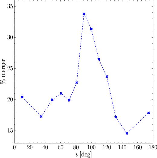
Merger fraction as a function of the initial relative inclination between the inner and outer binary. Post-ejection coalescences are not included. The prominent peak at ι ≈ 90° confirms the important role of the K–L mechanism in driving the merger of MBHBs.
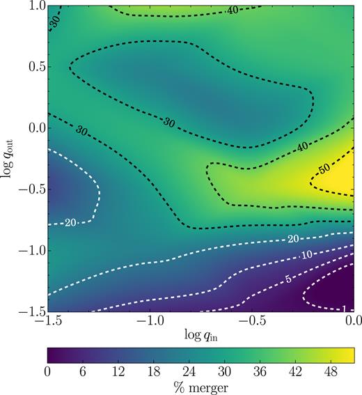
In a two-dimensional map (Fig. 3), we show again the merger fraction, but now as a function of the initial values of qin and qout.3 The peak of the merger fraction occurs for equal-mass triplets, but there is a large plateau in the upper part of the plot, with hints of two distinct maxima. A simple interpretation is that the inner binary, in order to be perturbed, needs to interact with an intruder of at least a comparable mass (i.e. log qout ≈ −0.3). A light m3 is most probably simply kicked out by the heavier inner binary, as hinted at by the rapid decline of the merger fraction as qout gets ≪1 (see Heggie 1975). Note, however, that even for low values of qout the merger fraction is significant when qin is also small (thus, when m2 ≈ m3).
![Merger fraction (colour coded) as a function of the inner (qin = m2/m1) and outer [qout = m3/(m1 + m2)] mass ratios. The merger fraction is larger (≳30 per cent) in the upper region, corresponding to qout ≳ 0.3 and 0.1 ≲ qin ≲ 1. The circles in the four corners of the plot represent, in cartoon-like fashion, the corresponding mass hierarchy of the triplets.](https://oup.silverchair-cdn.com/oup/backfile/Content_public/Journal/mnras/477/3/10.1093_mnras_sty896/1/m_sty896fig3.jpeg?Expires=1750340543&Signature=RfLW-6sKQNH5V-UomZkGrQ2MduMf9YzYoUHxvjNvl14yaChqkMknCVtjv4woM9wakI0mseO6k8~P3IKAItQ7dDBxLzt-Ax25l3Yt0cfhHZYf2bJVJ6weukCIRGFgwseJkopeU6PWx3le-uBQEKej2gt3kAitgd~QLV1be7Zj16euQ6qgMLxcDWP31Piz5lq3K3ApWMqVRHP~pBSADmSIoyURkFyljIE9dxZXEaxzoAW~ypMbGpVK6yNkiTEOwVC8mezX16PKVFlN2MsjpMxhFOK2R8X8XF7BzAFUS7~KrrsJ03TbvrG-n5BxlFCRLjJtTCHzsmroYbituISyW0jnrw__&Key-Pair-Id=APKAIE5G5CRDK6RD3PGA)
Merger fraction (colour coded) as a function of the inner (qin = m2/m1) and outer [qout = m3/(m1 + m2)] mass ratios. The merger fraction is larger (≳30 per cent) in the upper region, corresponding to qout ≳ 0.3 and 0.1 ≲ qin ≲ 1. The circles in the four corners of the plot represent, in cartoon-like fashion, the corresponding mass hierarchy of the triplets.
A finer understanding of the results of Fig. 3 can be gained by considering that, at the octupole level, the K–L oscillations are more easily triggered when the inner binary has a small mass ratio. In this case, the inner binary can merge when the triplet is still in the initial hierarchical phase, and the eccentricity growth responsible for the coalescence is primarily driven by secular processes. This is the cause of the leftmost peak in the merger fraction, indeed occurring for log qout ≈ −0.3 and log qin ≪ 0. A second channel to coalescence is represented by merger-inducing strong non-secular close encounters that the original inner binary experiences once the triplet becomes unstable. This happens for almost equal-mass triplets, i.e. when the intruder carries a mass sufficiently large to perturb the inner binary, but, at the same time, the K–L mechanism is not easily triggered. During the process, prior to coalescence, several exchanges4 may occur, and therefore the final merger does not necessarily involve the members of the original inner binary. This second channel is responsible for the rightmost peak of the merger fraction in Fig. 3.
In order to better understand the role played by these two different channels in the merger fraction, we separately analyse the systems in which no exchange occurs during the evolution, and the rest of the systems that, instead, experiences strong encounters, ultimately leading to one or more exchange events. In addition, we single out systems with initial inclination in the range (70° < ι < 110°), hence dividing our simulations into four subsets.
The relative merger fraction of these subsets (i.e. relative to the number of simulations performed in a particular inclination range) is shown in Fig. 4. Left-hand panels represent the systems in which no exchange occurs. In these cases, the coalescence is mainly due to secular K–L oscillations, a fact confirmed by the comparatively much higher merger fraction (factor of ≈ 3) at high initial inclinations (upper left-hand panel). Moreover, we note that low qin is more likely to lead to mergers, irrespective of the inclination. As already mentioned, this is to be ascribed to the octupole terms of the K–L resonances, whose amplitude is proportional to the mass difference m1 − m2, hence vanishing for qin → 1. Note that, unlike in the standard quadrupole K–L resonances, the introduction of the octupole terms can excite high eccentricities even at low inclinations, a fact responsible for the non-negligible merger fraction in the lower left-hand panel of Fig. 4. At high inclinations, the region of both low qout and low qin should be prone to the K–L mechanism, but our results show no significant merger fraction (Fig. 4, upper left-hand panel). This can be understood by noting that if the time-scale of the relativistic precession is shorter than that of the K–L oscillations, the latter are damped. Since the K–L time-scale increases as m3 decreases, in the limit qout ≪ 1 the process is largely suppressed by relativistic precession. The relatively large merger fraction visible in the lower left area of Fig. 3 is then due to non-secular processes.
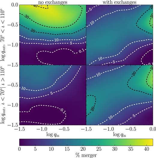
Break-up of Fig. 3 into different sub-populations. The two columns distinguish between merging binaries that underwent at least one close encounter leading to an exchange (right) and merging binaries that experienced no such encounters (left). The two rows identify sub-populations starting off with relative inclinations 70° < ι < 110° (top) and ι < 70° or ι > 110° (bottom). Merger fractions are normalized with respect to the total number of simulations in the respective inclination range.
The right-hand panels of Fig. 4 show the non-secular channel to merger. The first thing to notice is that the pattern of the merger fraction is almost independent of the inclination angle, consistent with the fact that exchanges occur when chaotic interactions take place and secular processes play no significant role. The merger fraction is larger when the three MBHs have similar masses, and in general has non-negligible values (>10 per cent) only along a broad-band stretching from the upper right to the lower left sides of the qin − qout plane. This can be understood by considering that when qin ≃ 1 and qout ≪ 1 (i.e. in the lower right corner of the plot), the intruder cannot perturb significantly the much more massive inner binary. On the other extreme (i.e. qin ≪ 1 and qout ≃ 1, upper left corner of the plot), m3 simply kicks the much lighter m2 out of the inner binary, taking its place. It is only when m3 ∼ m2 that genuinely chaotic dynamics can take place, in some cases leading to coalescence.
Finally, Fig. 5 shows the merger fraction as a function of the initial eccentricity of the inner and outer binary. We note that the merger fraction increases with increasing ein, while it decreases with increasing eout. The dependence upon ein is readily understood, since highly eccentric inner binaries are closer to the efficient GW-emission stage and can easily be driven to coalescence by a relatively mild perturbation from a third body. The dependence upon eout is likely due to the fact that quasi-circular outer binaries form a stable hierarchical triplet for a comparatively longer time during the inspiral of m3, hence leaving more room to the development of K–L resonances, which are efficient at driving the inner binary to coalescence. Conversely, in very eccentric outer binaries, m3 soon interacts with the inner binary at pericentre, entering the chaotic phase. Chaotic interactions are more likely to result in ejections rather than mergers, hence suppressing the overall merger fraction.
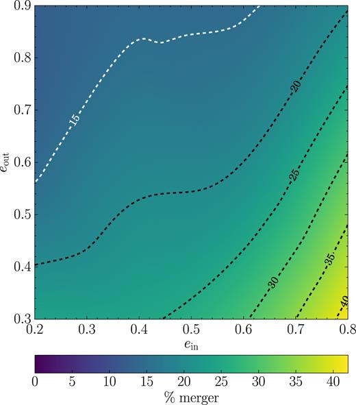
Merger fraction (colour coded) as a function of the initial inner (ein) and outer (eout) binary eccentricities.
3.1.1 Importance of PN corrections
As pointed out in the previous section, the K–L mechanism can be suppressed by general relativistic effects. In particular, relativistic precession tends to destroy the coherent pile-up of the perturbation that the third body induces on the inner binary, hence effectively damping the K–L resonances.5 In order to quantify the impact of the relativistic precession on the merger fraction and to compare our results with previous work that neglected this effect (e.g. Iwasawa, Funato & Makino 2006; Hoffman & Loeb 2007), in Table 3 and in Fig. 6 we compare, only for the case m1 = 109 M⊙, the merger fraction obtained with and without 1PN corrections. Overall, the merger fraction is substantially higher in the case without 1PN terms (right-hand panel of Fig. 6). As can be seen, the largest differences compared to the full case occur for qin ≪ 1, where, because of octupole-order terms, the K–L mechanism is maximally effective. On the contrary, for large qin the merger fractions with or without 1PN corrections are similar, because, as previously discussed, coalescences are mainly due to chaotic strong encounters, rather than to K–L oscillations. Our results highlight the importance of K–L resonances in inducing MBH mergers in triple systems, and the need to account at least for 1PN corrections.

Comparison between the merger fraction in the case m1 = 109 M⊙, when the dynamics is evolved with (left-hand panel) and without (right-hand panel) 1PN term. The suppression of the merger fraction for low qin, due to 1PN precession, is clearly visible (see discussion in the main text).
Comparison of the merger fraction from the simulations with m1 = 109 M⊙, run with and without conservative 1PN corrections.
| |$m_1 = 10^{9} \ \rm M_{{\odot }}$| | Per cent mergers including 1PN | Per cent mergers without 1PN | ||||||
|---|---|---|---|---|---|---|---|---|
| qin/qout | m1−m2 | m1−m3 | m2−m3 | Total | m1−m2 | m1−m3 | m2−m3 | Total |
| 0.0316/0.0316 | 9.0 | 5.1 | 0.0 | 14.1(20.5) | 44.2 | 5.8 | 0.0 | 50.0(5.1) |
| 0.0316/ 0.1 | 23.7 | 3.2 | 0.0 | 26.9(13.5) | 59.0 | 1.9 | 0.0 | 60.9(5.1) |
| 0.0316/0.3162 | 9.0 | 1.3 | 0.6 | 10.9(3.8) | 41.0 | 3.2 | 0.0 | 44.2(3.8) |
| 0.0316/ 1 | 25.0 | 0.0 | 1.9 | 26.9(0.0) | 62.2 | 0.0 | 0.6 | 62.8(0.0) |
| 0.1/0.0316 | 4.5 | 1.9 | 0.0 | 6.4(16.7) | 29.5 | 1.9 | 0.0 | 31.4(12.8) |
| 0.1/ 0.1 | 16.0 | 5.8 | 0.6 | 22.4(17.3) | 35.9 | 6.4 | 1.3 | 43.6(17.9) |
| 0.1/0.3162 | 24.4 | 3.2 | 1.3 | 28.8(11.5) | 44.9 | 4.5 | 0.6 | 50.0(7.7) |
| 0.1/ 1 | 25.6 | 0.0 | 7.1 | 32.7(1.3) | 40.4 | 0.6 | 7.7 | 48.7(0.0) |
| 0.3162/0.0316 | 2.6 | 0.6 | 0.0 | 3.2(7.1) | 9.0 | 0.0 | 0.6 | 9.6(5.8) |
| 0.3162/ 0.1 | 12.8 | 2.6 | 0.6 | 16.0(14.1) | 17.3 | 5.8 | 0.0 | 23.1(9.6) |
| 0.3162/0.3162 | 26.3 | 14.1 | 3.8 | 44.2(16.0) | 30.1 | 13.5 | 4.5 | 48.1(16.0) |
| 0.3162/ 1 | 17.3 | 1.9 | 4.5 | 23.7(5.8) | 29.5 | 3.2 | 5.8 | 38.5(6.4) |
| 1/0.0316 | 1.3 | 0.0 | 0.0 | 1.3(5.1) | 3.2 | 0.6 | 0.0 | 3.8(1.3) |
| 1/ 0.1 | 5.8 | 0.0 | 0.6 | 6.4(8.3) | 18.6 | 1.3 | 1.3 | 21.2(10.3) |
| 1/0.3162 | 26.9 | 12.2 | 14.1 | 53.2(16.0) | 33.3 | 9.6 | 6.4 | 49.4(13.5) |
| 1/ 1 | 13.5 | 14.1 | 15.4 | 42.9(21.8) | 19.9 | 16.0 | 18.6 | 54.5(11.5) |
| Average | 15.2 | 4.1 | 3.2 | 22.5(11.2) | 32.4 | 4.6 | 3.0 | 40.0(7.9) |
3.2 Merger time-scales
The time spent by triplets before coalescence is shown in Fig. 7. The merger-time distribution is remarkably well fitted by a lognormal, with a mean μ = 8.4 and a standard deviation σ = 0.4 in log (T/yr). The mean value μ = 8.4 corresponds to ≃ 250 Myr, i.e. a time-scale substantially shorter than the Hubble time, indicating that the triplet channel can lead to fast mergers. Indeed, most of the time prior to merger is spent in the dynamical friction and stellar hardening dominated regimes, i.e. most of the time the intruder is far from the inner binary. Once a genuinely bound triplet is formed, secular and (in some cases) chaotic interactions drive the system to coalescence on a much shorter time-scale.
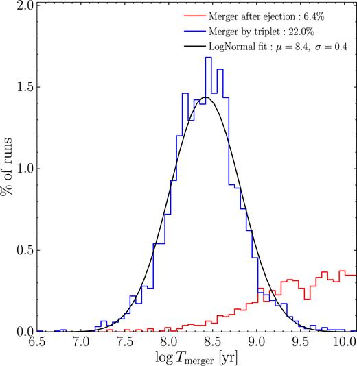
Distribution of merger-times. The blue histogram represents binaries that merge because of the prompt interaction with a third body (chaotic dynamics and/or K–L resonances plus GWs) and the black line is a lognormal fit to the distribution. The red histogram, instead, represents the binaries that are driven to merger by GW emission alone after the ejection of one of the MBHs (always the lightest one).
In Fig. 7 we also show, as a lower red histogram, the merger-time distribution of the ‘post-ejection’ coalescences discussed in Section 3.1. These events, which account for approximatively 1/5 of the total merger fraction and which are relatively more probable for high m1 values (see Table 2), involve an ejection, and a leftover inner binary that coalesces within a Hubble time under the effect of GW emission alone. The merger-time distribution is quite broad for these systems, and these MBHBs typically need a few Gyr to merge.
In Fig. 8 the merger-time distribution is shown for the different sampled values of qin (in the four panels) and qout (indicated by different colours in each panel). While there is no clear dependence of the merger time-scale on qin, we note a weak dependence on qout, with qout ≃ 1 systems coalescing faster because of the stronger perturbations exerted by m3 on the inner binary.
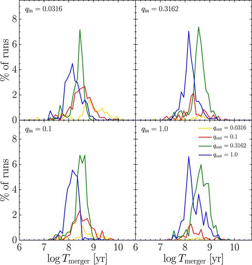
Distribution of merger-times, grouped according to the initial mass ratio of the inner (as labelled in the upper left corner of all panels) and outer binary (differentiated by colours as indicated in the lower right-hand panel). The merger time-scale only has a weak dependence on the outer mass ratio.
3.3 Eccentricity distribution
Of particular importance for GW emission from MBHBs in a cosmological setting is the study of the eccentricity evolution of merging binaries. In the left-hand panels of Fig. 9, we track the evolution of the merging binaries in the orbital frequency versus circularity plane (f, 1 − e), colour coding the probability of finding a binary at given values of eccentricity and frequency. We first discretize the [log f, log (1 − e)] space in the range −14 ≤ log f ≤ −2 and −4 ≤ log (1 − e) ≤ 0 on a 150 × 150 grid equally spaced along each direction. Then, we evaluate the time spent by each merging binary in each of the 22 500 bins of the grid during its evolution, then sum over all merging binaries, and normalize to the total time spent over all bins by all binaries. In this way, we obtain a bivariate normalized function that gives the probability of finding a binary in a given logarithmic two-dimensional interval of frequency and circularity. We construct this function for the six sampled values of m1, and show in Fig. 9, left-hand panels, three cases (m1 = 105, 107, 109 M⊙). The evolutionary tracks of single illustrative merging binaries are shown as a red line.
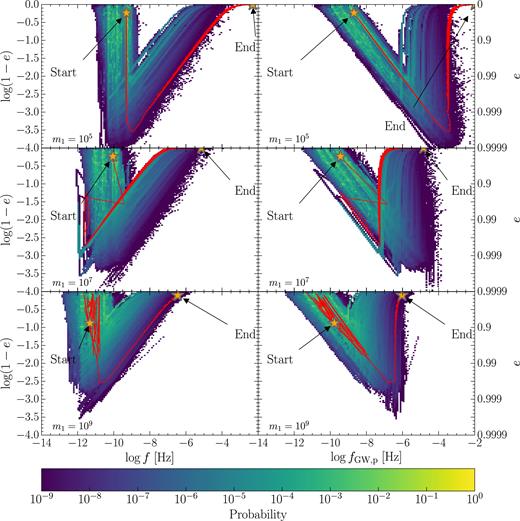
Evolution in the plane (f, 1 − e) (left-hand panels) and (fGW, p, 1 − e) (right-hand panels) of all merging binaries for three selected values of m1 = 105, 107, 109 M⊙ (from top to bottom). Colour coded is the probability (see the text for details about the computation) of finding a binary at given values of frequency and eccentricity. For each mass, superimposed in red is the evolutionary track of a representative binary that reached final coalescence. In the top panels such a representative binary merges when the triplet is still in the hierarchical phase, while in the lower panels the binary experiences strong chaotic three-body interactions, clearly visible in the noisy change of orbital elements. The primary effect of the triple interactions (secular or chaotic) is the great increase of the orbital eccentricity, leading one of the pairs in the triplet to coalescence.
In the orbital frequency–eccentricity plane, a typical stalled inner binary starts its evolution in the upper left-hand corner, i.e. at large separation (i.e. low f) and with an eccentricity given by one of the four values of ein that we sample (see Table 1). As soon as the perturbations due to the approaching third body become significant, the inner binary becomes more eccentric. If the system undergoes K–L resonances, the eccentricity actually oscillates on the K–L time-scale between high and low values (these oscillations are not visible in Fig. 9 due to the scale used), with a secular shift to higher values because of the perturbation exerted by an increasingly closer m3. The orbital frequency (i.e. the separation) of the inner binary stays nearly constant during this evolutionary phase. An example is given by the red line shown in the m1 = 105 M⊙ case (Fig. 9, upper left-hand panel). When chaotic interactions are instead the main driver of the binary evolution, f can show large, random variations, as exemplified by the tracks in the middle and lower left-hand panels of Fig. 9.
In any case, when the eccentricity becomes very high, ≳ 0.99, GW emissions start dominating the dynamics, increasing the orbital frequency and circularizing the orbit until coalescence, as can be seen from the rising branch of the red tracks. The colour code shows that this circularization phase is much shorter than the preceding evolution. The maximum eccentricity reached (the turnover point in the evolutionary tracks) mainly depends on the mass of the inner binary, i.e. the lower the mass, the higher the maximum eccentricity. In fact, for more massive binaries GWs start dominating sooner during the evolution, hence determining the earlier orbital circularization. This behaviour is clearly visible in Fig. 9, moving from the top panel (m1 = 105 M⊙) to the bottom one (m1 = 109 M⊙). Note that for more massive systems the orbital frequency at merger is necessarily lower, since it scales as M−1, where M ≡ m1 + m2.
During the initial phase of eccentricity growth, irrespective of the evolution driver (K–L resonances or chaotic interactions), the orbital frequency does not change (left-hand panels in Fig. 9), but fGW, p increases because of its dependence on e. As soon as GWs take over, the orbit circularizes fast while maintaining an almost constant fGW, p until the very last phase of the evolution. This means that during the circularization phase, the binaries maintain a fixed pericentre separation while their semimajor axis shrinks. Once the circularization is completed, GW losses keep shrinking the semimajor axis. Therefore, fGW, p increases and eventually becomes twice the orbital frequency (fGW, p = 2f), as expected for circular binaries at leading PN order. Like the orbital frequency, in the GW-dominated regime fGW, p is lower for larger masses.
A particularly interesting result of our simulations is that more massive binaries merge with a slightly larger eccentricity compared to their low mass counterparts, despite their maximum eccentricity being comparatively lower. This is essentially due to the shorter time-scale of the inspiral phase, which results in a sizeable residual eccentricity, as can be seen in Fig. 9 by observing the positions marked as ‘End’.
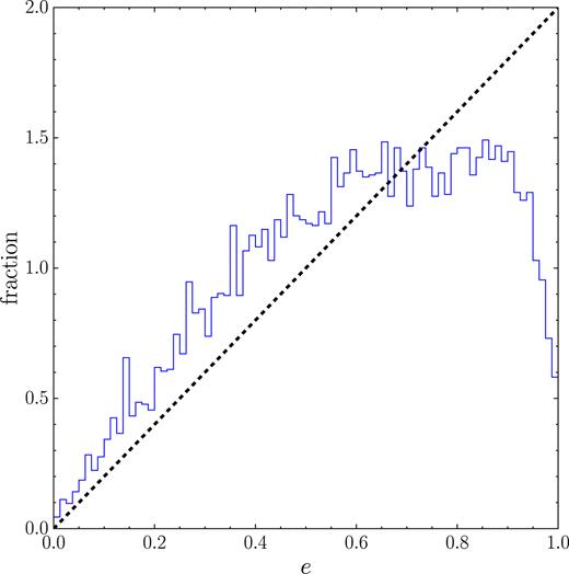
Fig. 10 shows the distribution of the eccentricity of merging MBHBs at an arbitrary spatial threshold corresponding to the last stable circular orbit of a non-spinning MBH with mass equal to the total binary mass, i.e. rISCO = 6RG with RG = GM/c2. In the left-hand panel, we plot the distribution on a linear scale, while in the right-hand panel we show the logarithmic version of the same distribution. It is remarkable that the distribution extends up to eISCO ≃ 0.1, as shown by the blue histogram.
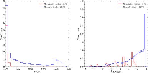
Distribution of eISCO of all merging binaries. Colour coded as in Fig. 7. The binaries that merge after a strong interaction with the third body retain a larger eccentricity close to merger compared to those that are GW-driven. Left-hand panel: linear scale. Right-hand panel: log scale. Note the peculiar clustering of the red distribution in six different blocks corresponding to the six different values of m1, i.e. from, left to right, 105 to 1010 M⊙.
In the same figure, the red histogram refers to the ‘post-ejection’ coalescences, which we recall account for ≃ 1/5 of the total. As expected, given that the final coalescence is purely driven by GW emission, these mergers are much less eccentric. Their low residual eccentricity has a marked dependence on the mass of the triplet, as can be inferred from the logarithmic version of the plot. Indeed, the right-hand panel of Fig. 10 shows that the eISCO distribution clusters around six different values, corresponding to the six values of m1 that we have sampled, with m1 increasing from left to right. Note that the distribution of eISCO for the mergers driven by triple interactions does not show any clustering, as expected in the case of coalescences induced by dynamical processes.
Finally, in Fig. 11, for different values of ein, we plot the eccentricity distribution of the inner binaries that did not merge within a Hubble time after the ejection of one of the three bodies. The distribution is approximatively thermal [i.e. p(e) ∝ e, see e.g. Jeans 1919; Heggie 1975, for further details] in the range from 0 ≲ e ≲ ein. This behaviour is typical of binaries that have experienced strong dynamical encounters during their evolution. The distribution shows a turnover at e ≳ ein, due to the fact that binaries with a higher eccentricity merge within a Hubble time, and are therefore not counted in the shown distribution. In Fig. 12 the same distribution is plotted summing over all ein. In this case, the slope results steeper than thermal because of the piling of binaries with low ein, which obey a thermal distribution only in a narrower range of e.
![Eccentricity distribution according to the initial value of ein, for those binaries that, after the ejection of one of the MBHs, do not merge within a Hubble time. The eccentricity approximately follows a thermal distribution [i.e. f(e) = 2e, represented as a black dashed line in the figure] in the range 0 ≲ e ≲ ein. At higher eccentricities the distribution shows a turnover, as some binaries are driven to coalescence (and therefore counted as mergers) by GW emission.](https://oup.silverchair-cdn.com/oup/backfile/Content_public/Journal/mnras/477/3/10.1093_mnras_sty896/1/m_sty896fig11.jpeg?Expires=1750340543&Signature=yTga8DkVHU8LEYay0ufudltL8DHBtQu9h~bQG3W~~OwT2UsaNW4-TYHR1zU-LbCPVJBaD7tGdJ0FAhoh37co6zCjMK3nCAxuliHzyPw3vshz1iPhB7FTnjL8Vgd3THC46eCe8ZQnfNMzpUDB8H-LZUDB2suBqlXLmkhpDKFZR0Bm4E81UzFSjwE~4ZBCpo2uHwjsG0ur0h3HWEXLdrJSyc-4WBB085h35qiWTcYPXx1eyr8ZSlQ90bKvo-Ed3RTuuitbRjZwuQXN3-54cQbpgXWmd5vOwRA9U1A5hveno746AzRyowMgpra9TgnEAsvl2I5zgabmL3tKaPhaVQ3z2A__&Key-Pair-Id=APKAIE5G5CRDK6RD3PGA)
Eccentricity distribution according to the initial value of ein, for those binaries that, after the ejection of one of the MBHs, do not merge within a Hubble time. The eccentricity approximately follows a thermal distribution [i.e. f(e) = 2e, represented as a black dashed line in the figure] in the range 0 ≲ e ≲ ein. At higher eccentricities the distribution shows a turnover, as some binaries are driven to coalescence (and therefore counted as mergers) by GW emission.
Same as Fig. 11, summing over all ein. Note that the slope is steeper than thermal because of the contribution of low ein.
4 DISCUSSION
4.1 Implications for the emission of GWs
The results presented in the previous section suggest that MBH triplets might have a critical impact on the emission and detection of low-frequency GWs. Although two forthcoming papers in this series are devoted to derive and analyse in depth the implications for LISA and PTAs separately, we preview here some relevant points.
The fact that about 30 per cent of triple systems lead to coalescence of an MBHB implies that this is an effective ‘last resort’ to overcome the final-parsec problem, should all other dynamical mechanisms fail. If the average galaxy undergoes a fairly large number of mergers during its cosmic history, then triple MBH interactions guarantee that a significant fraction of these galaxy mergers leads to an MBHB coalescence (see also Mikkola & Valtonen 1990; Heinämäki 2001; Blaes et al. 2002; Hoffman & Loeb 2007; Kulkarni & Loeb 2012). For example, under the simplifying assumption that the parameters of the forming triplets are uniformly distributed in the range explored in this study, this fraction is expected to be around 30 per cent. Therefore, compared to a scenario where MBHBs merge efficiently, the merger rate should be at most suppressed by a factor of ≃ 3. This is particularly encouraging for low-frequency GW probes. Indeed, even if MBHB stalling turns out to be a problem, LISA detection rates would be affected by a factor of ≃ 3 only, while the stochastic GW background in the PTA band would only be suppressed by a factor of|$\sqrt{3}$| (since the GW background is proportional to the square root of the number of mergers). Conversely, if the average galaxy undergoes ≲1 merger during its cosmic history, MBH triplets would not form frequently. In this scenario, MBHB stalling would result in a severe suppression of any low-frequency GW signals, posing a potential threat to PTAs and LISA. In the accompanying and forthcoming papers of the series, we will couple our library of simulations to a semi-analytic model for galaxy and MBH evolution, to explore which types of scenarios are more likely to occur in Nature, and to properly quantify the fraction of galaxy mergers resulting in MBHB coalescences.
Triple interactions also leave a distinctive imprint in the eccentricity distribution of merging MBHBs. In fact, whether secular processes or chaotic dynamics dominate the evolution, the coalescence is triggered when one of the MBH pairs is eccentric enough that a significant amount of GWs is emitted at subsequent pericentre passages. The net result is that triplet-induced MBHB coalescences typically involve eccentric systems. Even at separation ∼rISCO, eccentricity can still be as high as 0.1, and is ≳ 0.01 for more than 50 per cent of the binaries.
LISA is mostly sensitive to 105–106 M⊙ MBHBs throughout the Universe. Those systems typically enter the detector band at separations around 100RG. The cumulative eccentricity distribution of merging systems for all simulations with m1 = 105 M⊙ is shown in Fig. 13. Although skewed towards e = 0, the distribution extends to e ≈ 0.8, with about 30 per cent of the systems having e ≳ 0.5. Therefore, high eccentricities in the LISA band might be the smoking gun of triple-driven coalescences, and waveforms accurate up to high eccentricities might be necessary for proper recovery of the source parameters. Conversely, PTAs are sensitive to masses ≳ 108 M⊙ at low redshift. In Fig. 13 we also show the eccentricity distribution of merging systems for all simulations with m1 = 109 M⊙ at a separation of 1000RG, which is a representative of the sources dominating the GW signal in the nHz band. Note that the distribution extends to e ≈ 0.99, and about 50 per cent of the systems have eccentricity in excess of 0.9. Thus, in a universe dominated by triple interactions, the PTA signal is expected to be dominated by very eccentric binaries.
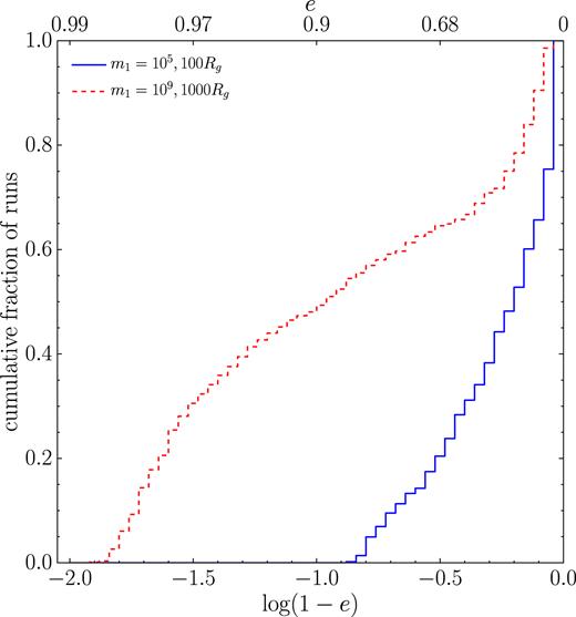
Cumulative distribution of 1 − e of all merging binaries with m1 = 105 M⊙ (blue solid line) and m1 = 109 M⊙ (red dashed line). In the case of m1 = 105 M⊙ (109 M⊙) the distribution is evaluated when the separation is 100 (1000) RG, most relevant for LISA (PTAs).
A further consequence of high eccentricities is the possibility of generating bursts of GWs. In practice, binaries with high e mostly emit GWs at every pericentre passage, resulting in a ‘burst signal’ well localized in time and spread (in frequency) over a large number of harmonics (Amaro-Seoane et al. 2010). As an example, massive binaries with orbital periods of hundreds of years can emit month-long bursts in the PTA frequency band, while lighter binaries with periods of several months can emit bursts detectable by LISA. This latter case is particularly interesting, because it might enhance the number of LISA detections well beyond the nominal MBHB merger rate. We will investigate this possibility in a forthcoming paper.
4.2 Effect of massive intruders
Although the inner mass ratio is qin ≤ 1 by definition, the outer mass ratio qout = m3/(m1 + m2) may be larger than one if the intruder is more massive than the bound binary. This can be relevant in a hierarchical structure-formation scenario, where a pre-existing stalled binary can be involved in a merger with a third, more MBH brought on by a galaxy merger. To explore the possible outcomes of this kind of configurations, we have run an additional set of simulations for the case m1 = 109 with qout = 3, 10. Although in this case one might expect the stellar potential to be dominated by the host galaxy of the intruder m3, we ignore this fact and simply centre the stellar potential in the (initial) centre of mass of the bound inner binary. This should not significantly affect the outcome of the simulation, at least qualitatively and in a statistical sense, since we find that the stellar potential has little effect on both the secular K–L evolution and the later chaotic phase (if present).
Results are shown in Fig. 14, where the original parameter space of Fig. 4 is extended up to qout = 10. As one might expect, the merger fraction stays quite high, around 30 per cent when qout ≳ 1. This is the result of two competing effects. On the one hand, the K–L time-scale is inversely proportional to m3/(m1 + m2); a massive intruder can therefore excite the eccentricity of the inner binary several times, favouring its prompt coalescence. On the other hand, at inclinations where K–L resonances are not very efficient, the unequal mass ratio favours the ejection of the lightest black hole, suppressing the fraction of systems that can merge in chaotic interactions. In any case, it is therefore important to take into account this kind of configurations when coupling libraries of triplet outcomes to semi-analytic galaxy-formation models, because they can have an impact on the global merger rate MBHBs.
Same as Fig. 3, but now extended up to qout = 10. Only the case m1 = 109 M⊙ is considered.
4.3 Comparison with previous work
We compare the results of the analysis of our simulations with the work of Hoffman & Loeb (2007), to which our investigation is similar in spirit, although we introduce some important novelties. The major differences are (i) the surveyed parameter space, which we extend to a wider range of masses, mass ratios, and initial eccentricities, (ii) our conservative choice of not considering a DM component, and (iii) the introduction of the conservative 1PN dynamics.
By comparing the merger fractions (their table 1 compared to our Table 2), we immediately note that their values are typically a factor of ≃ 3 larger than our results, even if ‘post-ejection’ merger binaries are added to our total. The discrepancy can be understood by analysing the differences in the two implementations:
All the simulations in Hoffman & Loeb (2007) have nearly the same total mass (≃6× 10⁸ M⊙), and moreover they considered systems, except in one case, in which the MBHs are nearly of equal mass. The interaction of nearly equal-mass objects produces the highest merger fraction, as can be seen from e.g. our Table 3 where in the nearly equal-mass case, the merger fraction is. In the only case in which Hoffman & Loeb (2007) consider a lower mass ratio, the merger fraction decreases below |$\lesssim 70\hbox{ per cent}$|, suggesting that the chosen mass ratio is in fact one of the reasons of the higher merger percentage. In practice, when restricting to comparable mass ratios, the merger fractions differ by less than a factor of ≃ 2 (|${\approx } \ 50\hbox{ per cent}$| versus).
The 1PN dynamics can further contribute to the difference. Even though it is mostly effective at low mass ratios (as can be appreciated from Fig. 6), the merger fraction can still be about 10 per cent higher even at comparable mass ratios when the 1PN relativistic precession is neglected.
The absence of a DM halo and the conservative threshold for MBH ejection assumed in our simulations also plays a role. As already discussed in Section 2, our choice implies that a larger number of MBHs are ejected, compared to Hoffman & Loeb (2007). This is confirmed by their run featuring a less massive DM halo, where the merger fraction drops to |${\sim } \ 70\hbox{ per cent}$|. As already discussed, our choice is meant to be conservative, in the sense that outside the stellar bulge significant triaxiality and asymmetries in the potential will likely prevent the ejected MBH from returning back to the centre (Guedes et al. 2009; Sijacki, Springel & Haehnelt 2011). We will explore this issue in greater detail in a future work.
In summary, we argue that the combination of the three points above fully explains the differences between the two studies.
5 CONCLUSIONS
In this study, we have utilized the three-body integrator presented in Bonetti et al. (2016) to investigate the outcome of MBH triple interactions over a vast parameter space. The code evolves the dynamics of MBH triplets including a variety of relevant factors, such as an external galactic potential, the dynamical friction against the stellar background, the stellar hardening, and the PN corrections to the equations of motion consistently derived from the three-body PN Hamiltonian. The set-up of the code is tuned to capture the physics relevant to three-body interactions of MBHs originated by repeated galaxy mergers in hierarchical cosmologies. We have explored the parameter space relevant to this specific context by considering primary MBH masses in the range 105 M⊙ ≤ m1 ≤ 1010 M⊙, a variety of inner and outer binary mass ratios in the range of 0.03−1, and several inner and outer binary initial eccentricities and mutual orbit inclinations as detailed in Table 1. We have integrated a grand total of 14 976 configurations with the goal of deriving the fraction of merging systems as a function of the relevant parameters, as well as the typical merger time-scales and properties of the coalescing MBHs.
Our main results can be summarized as follows:
The fraction of systems experiencing the merger of one of any pair of MBHs in the triplet is about 30 per cent. About 4/5 of these mergers are promptly induced during the three-body interaction, whereas about 1/5 are driven by GW emission following the ejection of the lightest black hole.
Prompt mergers are induced both by secular K–L evolution and chaotic dynamics. The former is more efficient for massive intruders (large qout) and eccentric inner binaries, while the latter is most efficient for nearly equal-mass systems. Overall, the merger fraction is higher for large qout, reaching 40 per cent of the systems.
The 1PN terms in the equations of motion are important at low qin/qout. Neglecting such correction, the fraction of low-q systems leading to a merger goes from |${\approx } \ 20\hbox{ per cent}$| to about |$40\hbox{ per cent}$|. This happens because 1PN precession destroys the K–L resonances, preventing the inner binary from reaching eccentricities high enough to merge under the effect of GW backreaction.
The typical time-scale for prompt mergers is well described by a lognormal distribution centred around |$\log (T/\rm yr)=8.4$| with a dispersion of 0.4 dex, almost independent of the masses and mass ratios involved. Note that this time-scale is dominated the orbital decay of the intruder, driven by dynamical friction and stellar hardening. Once the chaotic phase starts, mergers can be triggered within a few Myr Mergers following an MBH ejection occur on much longer time-scales, of the order of several Gyr
Merging binaries are generally driven to eccentricities in excess of 0.9 and up to 0.9999 in some cases, and even at coalescence binaries can retain a significant eccentricity, up to 0.1. Binaries driven by triple MBH interactions can therefore have eccentricities in excess of 0.5 when entering the LISA band, and in excess of 0.9 in the PTA frequency range.
Compared to the merger fractions found in previous studies (Hoffman & Loeb 2007), our numbers are significantly lower. This is because our parameter space includes lower mass ratios (which give a lower merger fraction), PN dynamics (which partially suppresses K–L resonances) and a conservative prescription for ejection (which does not include the galactic DM potential). Essentially, we consider an MBH as ejected forever once it reaches the outskirts of the stellar bulge. This is justified by the fact that triaxiality and potential asymmetries will likely prevent the MBH from sinking back to the centre in less than a few Gyr. In a future work, we plan to include a triaxial DM halo in our simulations, and study the impact on the MBHB merger fraction.
The aforementioned results indicate that MBH triplets can have a significant impact on MBH evolution and on future GW detections by LISA and PTAs. In particular, three-body interactions provide a partial solution to the final-parsec problem, even if all other binary shrinking mechanisms fail. This should guarantee a fairly large number of detectable GW sources, both by LISA and PTAs, regardless of the details of the interaction between MBHBs and their environment in galactic nuclei. In two papers, one accompanying and one forthcoming, we investigate this issue further by coupling our extensive library of MBH-triplet simulations to a state-of-the-art semi-analytic model of galaxy and MBH evolution.
Footnotes
See however Dvorkin & Barausse (2017) for the stochastic GW background under the hypothesis that all MBHBs stalled. That background, while suppressed relative to the case of efficient MBH mergers, would still be potentially observable by PTAs in the SKA era.
The choice about a minimum approach threshold is not an option, but a real requirement in the PN framework. Indeed, given its perturbative character, it is clear that as soon as two MBHs get sufficiently close, a full GR solution is needed to actually describe the merger event. Within the PN framework, we can safely describe the dynamics until the very last phases before the coalescence. Moreover, in order to avoid possible unphysical behaviours determined by a not sufficiently high PN dynamics (we have switched off the 2PN terms because of their huge computational cost), we have chosen such a conservative threshold.
Note that an equal-mass triplet (i.e. m1 = m2 = m3) is characterized by log qin = 0 and log qout = −0.3.
An exchange is an event in which the intruder kicks one body (usually the lightest one) out of the inner binary, and binds to the other to form a new two-body system.
More precisely, any kind of precession tends to suppress the K–L mechanism.
ACKNOWLEDGEMENTS
MB and FH acknowledge partial financial support from the INFN TEONGRAV-specific initiative. MB acknowledges the CINECA award under the ISCRA initiative, for the availability of high performance computing resources and support. This work was supported by the H2020-MSCA-RISE-2015 Grant No. StronGrHEP-690904. AS is supported by a University Research Fellowship of the Royal Society. This work has made use of the Horizon Cluster, hosted by the Institut d’Astrophysique de Paris. We thank Stephane Rouberol for running this cluster smoothly for us.
REFERENCES
APPENDIX: MERGER FRACTIONS
In this appendix, we report the tables of the merger fraction per range of m1 sliced according to various IC parameters, i.e. mass ratios, outer eccentricity, and initial relative inclination.
Results |$m_1=10^{10}\, \rm M_{{\odot }}$|.
| |$m_1 = 10^{10} \ \rm M_{{\odot }}$| | Per cent mergers | |||
|---|---|---|---|---|
| qin/qout | m1−m2 | m1−m3 | m2−m3 | Total |
| 0.0316/0.0316 | 21.2 | 9.6 | 0.0 | 30.8(32.7) |
| 0.0316/ 0.1 | 33.3 | 6.4 | 0.0 | 39.7(11.5) |
| 0.0316/0.3162 | 19.9 | 4.5 | 0.0 | 24.4(7.7) |
| 0.0316/ 1 | 32.1 | 1.3 | 5.8 | 39.1(7.7) |
| 0.1/0.0316 | 7.7 | 7.7 | 0.0 | 15.4(15.4) |
| 0.1/ 0.1 | 21.8 | 13.5 | 1.9 | 37.2(23.1) |
| 0.1/0.3162 | 36.5 | 8.3 | 3.2 | 48.1(10.3) |
| 0.1/ 1 | 18.6 | 4.5 | 4.5 | 27.6(7.1) |
| 0.3162/0.0316 | 4.5 | 1.3 | 0.0 | 5.8(10.9) |
| 0.3162/ 0.1 | 16.7 | 3.8 | 1.3 | 21.8(12.2) |
| 0.3162/0.3162 | 37.2 | 14.7 | 1.9 | 53.8(15.4) |
| 0.3162/ 1 | 19.2 | 7.7 | 7.1 | 34.0(7.1) |
| 1/0.0316 | 0.6 | 1.3 | 0.6 | 2.6(5.1) |
| 1/ 0.1 | 9.6 | 1.3 | 0.0 | 10.9(12.2) |
| 1/0.3162 | 32.7 | 16.7 | 10.9 | 60.3(9.6) |
| 1/ 1 | 25.6 | 18.6 | 15.4 | 59.6(14.7) |
| Average | 21.1 | 7.6 | 3.3 | 31.9(12.7) |
| ein/eout | m1−m2 | m1−m3 | m2−m3 | Total |
| 0.2/0.3 | 18.3 | 6.7 | 5.8 | 30.8(18.3) |
| 0.2/0.6 | 8.2 | 9.6 | 2.9 | 20.7(6.7) |
| 0.2/0.9 | 8.2 | 13.9 | 3.8 | 26.0(3.8) |
| 0.4/0.3 | 24.5 | 4.8 | 3.4 | 32.7(7.2) |
| 0.4/0.6 | 15.9 | 4.8 | 2.9 | 23.6(14.9) |
| 0.4/0.9 | 13.9 | 11.5 | 2.9 | 28.4(7.2) |
| 0.6/0.3 | 28.8 | 8.2 | 1.9 | 38.9(9.6) |
| 0.6/0.6 | 19.2 | 6.2 | 2.9 | 28.4(10.6) |
| 0.6/0.9 | 14.4 | 10.6 | 2.9 | 27.9(13.0) |
| 0.8/0.3 | 47.1 | 3.4 | 2.4 | 52.9(3.4) |
| 0.8/0.6 | 32.7 | 4.3 | 3.4 | 40.4(7.7) |
| 0.8/0.9 | 21.6 | 6.7 | 4.3 | 32.7(5.8) |
| Average | 21.1 | 7.6 | 3.3 | 31.9(12.7) |
| ι | m1−m2 | m1−m3 | m2−m3 | Total |
| 10 | 14.6 | 9.4 | 7.8 | 31.8(14.1) |
| 34.9323 | 11.5 | 8.9 | 3.6 | 24.0(14.6) |
| 49.0917 | 16.7 | 7.3 | 4.2 | 28.1(12.0) |
| 60.6678 | 20.8 | 7.8 | 2.1 | 30.7(14.6) |
| 71.0409 | 23.4 | 9.4 | 3.6 | 36.5(10.4) |
| 80.7981 | 23.4 | 8.9 | 3.6 | 35.9(12.5) |
| 90.2902 | 29.7 | 6.2 | 2.1 | 38.0(12.5) |
| 99.7903 | 33.9 | 4.7 | 2.6 | 41.1(10.9) |
| 109.574 | 27.1 | 6.2 | 1.0 | 34.4(12.0) |
| 120 | 25.5 | 5.7 | 1.6 | 32.8(15.1) |
| 131.681 | 13.5 | 9.9 | 2.1 | 25.5(9.9) |
| 146.094 | 15.1 | 5.7 | 3.6 | 24.5(12.0) |
| 174.231 | 18.8 | 8.3 | 4.7 | 31.8(14.1) |
| Average | 21.1 | 7.6 | 3.3 | 31.9(12.7) |
Results |$m_1=10^{9}\, \rm M_{{\odot }}$|.
| |$m_1 = 10^{9} \ \rm M_{{\odot }}$| | Per cent mergers | |||
|---|---|---|---|---|
| qin/qout | m1−m2 | m1−m3 | m2−m3 | Total |
| 0.0316/0.0316 | 9.0 | 5.1 | 0.0 | 14.1(20.5) |
| 0.0316/ 0.1 | 23.7 | 3.2 | 0.0 | 26.9(13.5) |
| 0.0316/0.3162 | 9.0 | 1.3 | 0.6 | 10.9(3.8) |
| 0.0316/ 1 | 25.0 | 0.0 | 1.9 | 26.9(0.0) |
| 0.1/0.0316 | 4.5 | 1.9 | 0.0 | 6.4(16.7) |
| 0.1/ 0.1 | 16.0 | 5.8 | 0.6 | 22.4(17.3) |
| 0.1/0.3162 | 24.4 | 3.2 | 1.3 | 28.8(11.5) |
| 0.1/ 1 | 25.6 | 0.0 | 7.1 | 32.7(1.3) |
| 0.3162/0.0316 | 2.6 | 0.6 | 0.0 | 3.2(7.1) |
| 0.3162/ 0.1 | 12.8 | 2.6 | 0.6 | 16.0(14.1) |
| 0.3162/0.3162 | 26.3 | 14.1 | 3.8 | 44.2(16.0) |
| 0.3162/ 1 | 17.3 | 1.9 | 4.5 | 23.7(5.8) |
| 1/0.0316 | 1.3 | 0.0 | 0.0 | 1.3(5.1) |
| 1/ 0.1 | 5.8 | 0.0 | 0.6 | 6.4(8.3) |
| 1/0.3162 | 26.9 | 12.2 | 14.1 | 53.2(16.0) |
| 1/ 1 | 13.5 | 14.1 | 15.4 | 42.9(21.8) |
| Average | 15.2 | 4.1 | 3.2 | 22.5(11.2) |
| ein/eout | m1−m2 | m1−m3 | m2−m3 | Total |
| 0.2/0.3 | 18.3 | 3.8 | 3.4 | 25.5(9.1) |
| 0.2/0.6 | 7.7 | 3.8 | 3.4 | 14.9(8.7) |
| 0.2/0.9 | 5.3 | 5.3 | 2.4 | 13.0(2.4) |
| 0.4/0.3 | 16.3 | 3.4 | 3.8 | 23.6(13.5) |
| 0.4/0.6 | 13.0 | 3.8 | 2.4 | 19.2(12.0) |
| 0.4/0.9 | 7.7 | 5.3 | 3.4 | 16.3(8.2) |
| 0.6/0.3 | 22.6 | 2.4 | 6.2 | 31.2(6.2) |
| 0.6/0.6 | 12.0 | 5.3 | 2.9 | 20.2(11.1) |
| 0.6/0.9 | 9.1 | 3.8 | 1.0 | 13.9(13.0) |
| 0.8/0.3 | 34.1 | 1.9 | 1.9 | 38.0(5.3) |
| 0.8/0.6 | 24.5 | 4.3 | 4.3 | 33.2(7.2) |
| 0.8/0.9 | 12.0 | 6.2 | 2.9 | 21.2(13.0) |
| Average | 15.2 | 4.1 | 3.2 | 22.5(11.2) |
| ι | m1−m2 | m1−m3 | m2−m3 | Total |
| 10 | 10.9 | 4.2 | 6.2 | 21.4(14.6) |
| 34.9323 | 10.4 | 4.2 | 3.1 | 17.7(10.4) |
| 49.0917 | 10.4 | 1.6 | 7.8 | 19.8(14.1) |
| 60.6678 | 10.4 | 2.1 | 7.3 | 19.8(13.0) |
| 71.0409 | 8.3 | 5.7 | 3.6 | 17.7(8.3) |
| 80.7981 | 17.7 | 6.2 | 0.5 | 24.5(12.5) |
| 90.2902 | 26.6 | 6.2 | 1.0 | 33.9(8.3) |
| 99.7903 | 27.1 | 2.1 | 1.0 | 30.2(8.9) |
| 109.574 | 18.2 | 4.7 | 0.5 | 23.4(12.5) |
| 120 | 22.4 | 2.6 | 3.1 | 28.1(13.0) |
| 131.681 | 14.1 | 4.2 | 1.0 | 19.3(8.9) |
| 146.094 | 10.4 | 5.2 | 2.1 | 17.7(10.9) |
| 174.231 | 10.9 | 4.7 | 3.6 | 19.3(9.9) |
| Average | 15.2 | 4.1 | 3.2 | 22.5(11.2) |
Results |$m_1=10^{8}\, \rm M_{{\odot }}$|.
| |$m_1 = 10^{8} \ \rm M_{{\odot }}$| | Per cent mergers | |||
|---|---|---|---|---|
| qin/qout | m1−m2 | m1−m3 | m2−m3 | Total |
| 0.0316/0.0316 | 9.6 | 8.3 | 0.0 | 17.9(5.1) |
| 0.0316/ 0.1 | 14.1 | 2.6 | 0.0 | 16.7(8.3) |
| 0.0316/0.3162 | 28.2 | 0.6 | 0.6 | 29.5(1.9) |
| 0.0316/ 1 | 14.7 | 1.3 | 2.6 | 18.6(3.2) |
| 0.1/0.0316 | 4.5 | 3.2 | 0.0 | 7.7(5.8) |
| 0.1/ 0.1 | 9.6 | 6.4 | 0.0 | 16.0(12.8) |
| 0.1/0.3162 | 22.4 | 6.4 | 1.3 | 30.1(5.1) |
| 0.1/ 1 | 21.8 | 0.0 | 1.9 | 23.7(2.6) |
| 0.3162/0.0316 | 1.3 | 1.3 | 0.0 | 2.6(3.2) |
| 0.3162/ 0.1 | 10.3 | 1.3 | 0.6 | 12.2(7.1) |
| 0.3162/0.3162 | 25.6 | 9.0 | 1.9 | 36.5(11.5) |
| 0.3162/ 1 | 23.1 | 3.2 | 8.3 | 34.6(5.1) |
| 1/0.0316 | 0.0 | 0.6 | 0.0 | 0.6(3.2) |
| 1/ 0.1 | 5.8 | 0.0 | 0.0 | 5.8(5.1) |
| 1/0.3162 | 25.0 | 9.6 | 10.9 | 45.5(11.5) |
| 1/ 1 | 19.2 | 10.3 | 11.5 | 41.0(9.0) |
| Average | 14.7 | 4.0 | 2.5 | 21.2(6.3) |
| ein/eout | m1−m2 | m1−m3 | m2−m3 | Total |
| 0.2/0.3 | 15.9 | 4.3 | 4.8 | 25.0(3.4) |
| 0.2/0.6 | 12.0 | 4.3 | 3.4 | 19.7(6.2) |
| 0.2/0.9 | 4.3 | 3.8 | 2.4 | 10.6(2.4) |
| 0.4/0.3 | 18.3 | 3.4 | 1.9 | 23.6(5.3) |
| 0.4/0.6 | 14.9 | 4.8 | 1.4 | 21.2(11.1) |
| 0.4/0.9 | 4.8 | 5.8 | 2.9 | 13.5(5.3) |
| 0.6/0.3 | 20.7 | 2.9 | 1.4 | 25.0(1.4) |
| 0.6/0.6 | 13.0 | 3.8 | 1.4 | 18.3(4.3) |
| 0.6/0.9 | 3.4 | 5.3 | 2.9 | 11.5(1.4) |
| 0.8/0.3 | 34.6 | 1.4 | 2.4 | 38.5(1.0) |
| 0.8/0.6 | 23.6 | 4.3 | 1.9 | 29.8(2.4) |
| 0.8/0.9 | 11.1 | 3.8 | 2.9 | 17.8(5.8) |
| Average | 14.7 | 4.0 | 2.5 | 21.2(6.3) |
| ι | m1−m2 | m1−m3 | m2−m3 | Total |
| 10 | 10.4 | 3.1 | 3.6 | 17.2(6.8) |
| 34.9323 | 8.9 | 3.1 | 3.1 | 15.1(6.2) |
| 49.0917 | 6.8 | 5.2 | 4.2 | 16.1(8.3) |
| 60.6678 | 13.0 | 5.7 | 2.6 | 21.4(4.7) |
| 71.0409 | 11.5 | 3.1 | 2.6 | 17.2(8.9) |
| 80.7981 | 14.6 | 2.6 | 4.2 | 21.4(6.8) |
| 90.2902 | 27.6 | 0.5 | 1.6 | 29.7(3.1) |
| 99.7903 | 28.1 | 2.1 | 1.0 | 31.2(3.1) |
| 109.574 | 20.3 | 4.2 | 2.1 | 26.6(6.8) |
| 120 | 19.3 | 2.6 | 1.6 | 23.4(5.2) |
| 131.681 | 13.5 | 4.2 | 2.1 | 19.8(5.2) |
| 146.094 | 7.8 | 7.3 | 0.0 | 15.1(8.9) |
| 174.231 | 9.4 | 8.3 | 3.6 | 21.4(7.8) |
| Average | 14.7 | 4.0 | 2.5 | 21.2(6.3) |
Results |$m_1=10^{7}\, \rm M_{{\odot }}$|.
| |$m_1 = 10^{7} \ \rm M_{{\odot }}$| | per cent Mergers | |||
|---|---|---|---|---|
| qin/qout | m1−m2 | m1−m3 | m2−m3 | Total |
| 0.0316/0.0316 | 5.1 | 4.5 | 0.0 | 9.6(6.4) |
| 0.0316/ 0.1 | 23.1 | 1.9 | 0.0 | 25.0(1.9) |
| 0.0316/0.3162 | 23.7 | 3.2 | 0.6 | 27.6(7.7) |
| 0.0316/ 1 | 23.7 | 5.8 | 0.0 | 29.5(1.9) |
| 0.1/0.0316 | 3.2 | 0.6 | 0.0 | 3.8(3.2) |
| 0.1/ 0.1 | 9.6 | 2.6 | 0.0 | 12.2(6.4) |
| 0.1/0.3162 | 32.1 | 1.3 | 0.6 | 34.0(5.1) |
| 0.1/ 1 | 22.4 | 1.9 | 0.6 | 25.0(3.2) |
| 0.3162/0.0316 | 0.0 | 0.6 | 0.0 | 0.6(0.6) |
| 0.3162/ 0.1 | 10.3 | 0.0 | 1.3 | 11.5(5.8) |
| 0.3162/0.3162 | 23.1 | 6.4 | 0.6 | 30.1(4.5) |
| 0.3162/ 1 | 23.1 | 0.0 | 7.1 | 30.1(0.6) |
| 1/0.0316 | 1.3 | 0.0 | 0.0 | 1.3(0.6) |
| 1/ 0.1 | 6.4 | 1.3 | 0.6 | 8.3(2.6) |
| 1/0.3162 | 24.4 | 3.8 | 5.1 | 33.3(9.0) |
| 1/ 1 | 14.7 | 6.4 | 6.4 | 27.6(11.5) |
| Average | 15.4 | 2.5 | 1.4 | 19.4(4.4) |
| ein/eout | m1−m2 | m1−m3 | m2−m3 | Total |
| 0.2/0.3 | 18.8 | 2.4 | 2.4 | 23.6(2.4) |
| 0.2/0.6 | 6.7 | 2.4 | 1.9 | 11.1(0.0) |
| 0.2/0.9 | 3.4 | 4.8 | 1.4 | 9.6 (1.4) |
| 0.4/0.3 | 21.6 | 1.4 | 2.4 | 25.5(3.8) |
| 0.4/0.6 | 13.9 | 1.0 | 1.0 | 15.9(6.2) |
| 0.4/0.9 | 5.8 | 2.9 | 1.4 | 10.1(4.8) |
| 0.6/0.3 | 21.6 | 2.4 | 1.0 | 25.0(1.4) |
| 0.6/0.6 | 13.5 | 1.9 | 1.9 | 17.3(5.8) |
| 0.6/0.9 | 8.7 | 2.9 | 0.5 | 12.0(3.8) |
| 0.8/0.3 | 39.4 | 0.5 | 0.5 | 40.4(1.4) |
| 0.8/0.6 | 22.6 | 4.8 | 1.4 | 28.8(1.9) |
| 0.8/0.9 | 8.7 | 2.9 | 1.4 | 13.0(4.3) |
| Average | 15.4 | 2.5 | 1.4 | 19.4(4.4) |
| ι | m1−m2 | m1−m3 | m2−m3 | Total |
| 10 | 12.5 | 2.6 | 1.6 | 16.7(5.7) |
| 34.9323 | 10.4 | 1.0 | 2.1 | 13.5(6.8) |
| 49.0917 | 12.0 | 2.1 | 3.1 | 17.2(3.6) |
| 60.6678 | 11.5 | 3.1 | 1.6 | 16.1(4.7) |
| 71.0409 | 14.6 | 2.6 | 1.6 | 18.8(5.2) |
| 80.7981 | 14.1 | 4.2 | 1.0 | 19.3(4.7) |
| 90.2902 | 31.2 | 1.6 | 1.0 | 33.9(3.6) |
| 99.7903 | 26.0 | 1.0 | 1.0 | 28.1(3.1) |
| 109.574 | 24.0 | 3.6 | 0.0 | 27.6(2.6) |
| 120 | 17.2 | 1.6 | 1.0 | 19.8(4.7) |
| 131.681 | 11.5 | 2.1 | 1.6 | 15.1(4.2) |
| 146.094 | 8.3 | 3.6 | 1.0 | 13.0(4.2) |
| 174.231 | 6.8 | 3.6 | 2.1 | 12.5(4.7) |
| Average | 15.4 | 2.5 | 1.4 | 19.4(4.4) |
Results |$m_1=10^{6}\, \rm M_{{\odot }}$|.
| |$m_1 = 10^{6} \ \rm M_{{\odot }}$| | per cent Mergers | |||
|---|---|---|---|---|
| qin/qout | m1−m2 | m1−m3 | m2−m3 | Total |
| 0.0316/0.0316 | 4.5 | 0.6 | 0.0 | 5.1(1.3) |
| 0.0316/ 0.1 | 11.5 | 0.0 | 0.0 | 11.5(0.0) |
| 0.0316/0.3162 | 25.6 | 0.0 | 0.0 | 25.6(2.6) |
| 0.0316/ 1 | 39.7 | 0.0 | 1.9 | 41.7(0.6) |
| 0.1/0.0316 | 1.3 | 0.6 | 0.0 | 1.9(1.9) |
| 0.1/ 0.1 | 9.0 | 1.3 | 0.0 | 10.3(6.4) |
| 0.1/0.3162 | 38.5 | 0.0 | 0.0 | 38.5(2.6) |
| 0.1/ 1 | 43.6 | 0.0 | 0.6 | 44.2(0.6) |
| 0.3162/0.0316 | 0.6 | 0.6 | 0.0 | 1.3(1.3) |
| 0.3162/ 0.1 | 3.2 | 0.6 | 0.0 | 3.8(0.0) |
| 0.3162/0.3162 | 19.9 | 1.3 | 0.0 | 21.2(1.9) |
| 0.3162/ 1 | 26.3 | 1.3 | 2.6 | 30.1(1.9) |
| 1/0.0316 | 0.6 | 0.0 | 0.0 | 0.6(0.6) |
| 1/ 0.1 | 1.9 | 0.6 | 0.6 | 3.2(1.3) |
| 1/0.3162 | 17.9 | 6.4 | 4.5 | 28.8(5.1) |
| 1/ 1 | 14.7 | 8.3 | 5.8 | 28.8(1.9) |
| Average | 16.2 | 1.4 | 1.0 | 18.5(1.9) |
| ein/eout | m1−m2 | m1−m3 | m2−m3 | Total |
| 0.2/0.3 | 16.3 | 2.9 | 1.4 | 20.7(1.4) |
| 0.2/0.6 | 6.7 | 0.5 | 0.5 | 7.7 (1.4) |
| 0.2/0.9 | 6.2 | 1.0 | 1.4 | 8.7 (3.4) |
| 0.4/0.3 | 18.8 | 1.4 | 1.4 | 21.6(1.9) |
| 0.4/0.6 | 14.4 | 1.4 | 1.9 | 17.8(3.4) |
| 0.4/0.9 | 7.7 | 1.0 | 1.0 | 9.6 (3.4) |
| 0.6/0.3 | 27.4 | 0.5 | 0.5 | 28.4(0.0) |
| 0.6/0.6 | 13.9 | 2.4 | 0.0 | 16.3(0.0) |
| 0.6/0.9 | 9.1 | 1.4 | 0.5 | 11.1(0.0) |
| 0.8/0.3 | 38.0 | 1.4 | 1.4 | 40.9(0.0) |
| 0.8/0.6 | 22.6 | 0.5 | 0.5 | 23.6(0.0) |
| 0.8/0.9 | 13.0 | 1.9 | 1.4 | 16.3(0.5) |
| Average | 16.2 | 1.4 | 1.0 | 18.5(1.9) |
| ι | m1−m2 | m1−m3 | m2−m3 | Total |
| 10 | 13.0 | 3.1 | 1.0 | 17.2(3.6) |
| 34.9323 | 13.5 | 0.0 | 2.1 | 15.6(1.6) |
| 49.0917 | 15.6 | 2.1 | 1.0 | 18.8(1.0) |
| 60.6678 | 17.7 | 0.5 | 1.6 | 19.8(2.6) |
| 71.0409 | 14.1 | 0.5 | 1.0 | 15.6(1.6) |
| 80.7981 | 18.2 | 0.5 | 0.0 | 18.8(1.6) |
| 90.2902 | 33.3 | 0.5 | 0.5 | 34.4(0.5) |
| 99.7903 | 25.5 | 0.5 | 0.0 | 26.0(1.6) |
| 109.574 | 20.3 | 1.0 | 0.5 | 21.9(2.1) |
| 120 | 15.6 | 2.6 | 1.6 | 19.8(0.5) |
| 131.681 | 9.9 | 1.6 | 0.0 | 11.5(4.2) |
| 146.094 | 5.7 | 1.6 | 3.1 | 10.4(1.0) |
| 174.231 | 7.8 | 3.1 | 0.5 | 11.5(2.6) |
| Average | 16.2 | 1.4 | 1.0 | 18.5(1.9) |
Results |$m_1=10^{5}\, \rm M_{{\odot }}$|.
| |$m_1 = 10^{5} \ \rm M_{{\odot }}$| | Per cent mergers | |||
|---|---|---|---|---|
| qin/qout | m1−m2 | m1−m3 | m2−m3 | Total |
| 0.0316/0.0316 | 1.9 | 1.9 | 0.0 | 3.8(2.6) |
| 0.0316/ 0.1 | 19.2 | 1.3 | 0.0 | 20.5(0.0) |
| 0.0316/0.3162 | 34.6 | 0.0 | 0.0 | 34.6(1.3) |
| 0.0316/ 1 | 23.1 | 0.0 | 1.3 | 24.4(3.8) |
| 0.1/0.0316 | 0.6 | 0.0 | 0.0 | 0.6(1.3) |
| 0.1/ 0.1 | 8.3 | 0.6 | 0.6 | 9.6(3.2) |
| 0.1/0.3162 | 35.3 | 0.6 | 0.0 | 35.9(1.3) |
| 0.1/ 1 | 40.4 | 0.0 | 0.0 | 40.4(0.0) |
| 0.3162/0.0316 | 1.9 | 0.0 | 0.0 | 1.9(0.0) |
| 0.3162/ 0.1 | 2.6 | 0.6 | 0.0 | 3.2(3.8) |
| 0.3162/0.3162 | 28.2 | 0.6 | 0.6 | 29.5(3.2) |
| 0.3162/ 1 | 30.8 | 0.6 | 3.8 | 35.3(0.0) |
| 1/0.0316 | 0.0 | 0.0 | 0.0 | 0.0(0.6) |
| 1/ 0.1 | 5.8 | 0.0 | 0.0 | 5.8(1.3) |
| 1/0.3162 | 19.2 | 3.8 | 5.1 | 28.2(2.6) |
| 1/ 1 | 16.7 | 4.5 | 1.9 | 23.1(1.3) |
| Average | 16.8 | 0.9 | 0.8 | 18.5(1.6) |
| ein/eout | m1−m2 | m1−m3 | m2−m3 | Total |
| 0.2/0.3 | 17.3 | 0.5 | 1.4 | 19.2(1.0) |
| 0.2/0.6 | 10.1 | 0.5 | 0.5 | 11.1(0.5) |
| 0.2/0.9 | 2.9 | 1.9 | 1.0 | 5.8 (1.4) |
| 0.4/0.3 | 17.8 | 0.0 | 1.9 | 19.7(0.5) |
| 0.4/0.6 | 12.5 | 1.4 | 1.0 | 14.9(1.4) |
| 0.4/0.9 | 6.7 | 1.0 | 0.5 | 8.2 (1.4) |
| 0.6/0.3 | 26.4 | 1.4 | 1.0 | 28.8(0.5) |
| 0.6/0.6 | 18.8 | 0.5 | 0.5 | 19.7(1.0) |
| 0.6/0.9 | 10.1 | 0.5 | 0.5 | 11.1(2.4) |
| 0.8/0.3 | 38.5 | 0.0 | 0.5 | 38.9(1.0) |
| 0.8/0.6 | 26.0 | 1.0 | 1.0 | 27.9(1.4) |
| 0.8/0.9 | 14.4 | 2.4 | 0.5 | 17.3(2.4) |
| Average | 16.8 | 0.9 | 0.8 | 18.5(1.6) |
| ι | m1−m2 | m1−m3 | m2−m3 | Total |
| 10 | 16.7 | 0.0 | 1.6 | 18.2(3.1) |
| 34.9323 | 15.6 | 1.6 | 0.5 | 17.7(2.6) |
| 49.0917 | 18.2 | 0.0 | 1.6 | 19.8(1.6) |
| 60.6678 | 15.1 | 0.5 | 2.6 | 18.2(1.6) |
| 71.0409 | 12.5 | 0.5 | 0.5 | 13.5(2.6) |
| 80.7981 | 16.1 | 0.0 | 0.5 | 16.7(1.0) |
| 90.2902 | 31.8 | 0.5 | 0.5 | 32.8(1.6) |
| 99.7903 | 30.7 | 0.5 | 0.0 | 31.2(1.0) |
| 109.574 | 21.4 | 1.6 | 2.1 | 25.0(1.0) |
| 120 | 17.7 | 0.5 | 0.0 | 18.2(1.0) |
| 131.681 | 9.9 | 1.6 | 0.5 | 12.0(0.5) |
| 146.094 | 5.2 | 1.6 | 0.0 | 6.8(2.1) |
| 174.231 | 7.3 | 3.1 | 0.5 | 10.9(1.6) |
| Average | 16.8 | 0.9 | 0.8 | 18.5(1.6) |
