


Abstract
We analyse the idea that the local dips (∼1 kpc along the Galactic radius) observed in oxygen abundance are associated with the infall of intergalactic low-abundant gas (∼0.2 Z⊙) on to the Galactic disc during the last ∼100 Myr. We term such infall events local streams. The derived masses of the falling gas (of the order of several times 108 M⊙) are close to the observed ones (e.g. in the Magellanic Stream). Such local streams do not change the mean mass of oxygen ejected per core-collapse supernova (CC SN) event, so that our previous inference on probable upper initial masses for progenitors of CC SNe remains valid.
1 INTRODUCTION
Using the new, most extensive data yet on oxygen abundances in Cepheids, as derived by Luck & Lambert (2011), Luck et al. (2013), Korotin et al. (2014) and Martin et al. (2015; for brevity hereafter we refer to these papers as 4KMLL), Mishurov & Tkachenko (2018; hereafter MT18) constructed the binned radial oxygen distribution along the Galactocentric radius r, averaging oxygen abundances within bins of size 0.5 kpc. Their binned radial oxygen distribution is shown in Fig. 1. The main feature of the pattern is the multislope radial gradient of the oxygen distribution: in the regions 5 ≲ r ≲ 7 kpc and 9 ≲ r ≲ 14 kpc the gradient is negative, whereas within 7 ≲ r ≲ 9 kpc the distribution is plateau-like. As shown in MT18, the formation of the aforementioned non-trivial regular pattern is associated with the combined effect of the corotation resonance and turbulent oxygen diffusion.
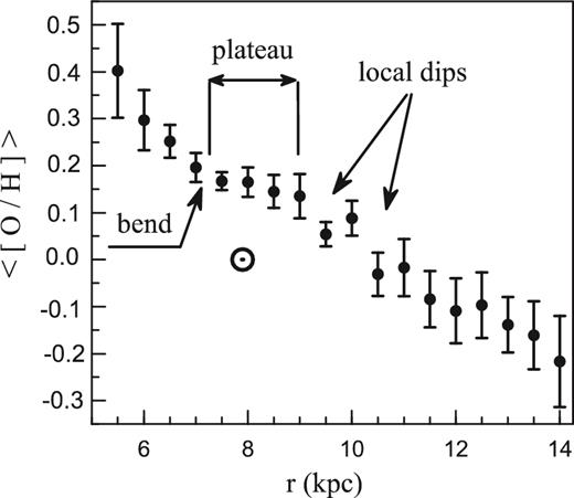
The filled circles and error-like bars are the binned radial oxygen abundances and their standard deviations along the Galactic radius constructed using abundances in Cepheids from 4MKLL. The solar symbol corresponds to the solar abundance. The locations of the ‘local dips’ discussed in the text are marked by arrows.
Fig. 1, however, displays a number of peculiarities, namely local depressions in the oxygen abundance at r ∼ 9.5 and 10.5 kpc of radial width ∼1 kpc. We refer to these features as ‘local dips’. Unlike the aforementioned regular pattern, the phenomenon of local dips may be associated with sporadic falls of the low-abundant intergalactic gas on to the disc at the epoch closest to the present time. There is nothing unusual in such a supposition, because infall clouds are well known (e.g. for high-velocity clouds, the Magellanic or Sagittarius Streams, clouds of ionized gas; see Lehner & Howk 2011; D'Onghia & Fox 2016, and references therein).
A priori, it is not obvious that this mechanism is able to explain the phenomenon of local dips. Indeed, the infall gas may increase the birth rate of progenitors for exploding core-collapse supernovae (CC SNe), which are the main source of oxygen, and thus clouds may produce an increase, rather than a decrease, in the oxygen abundance.
The aim of the present paper is to clarify whether this mechanism explains the phenomenon of the aforementioned local dips in the Galactic oxygen abundance.
2 MODEL FOR THE FORMATION OF LOCAL DIPS
In what follows, for the unperturbed stage (i.e. t ≤ TD − δt) we adopt all quantities from MT18. But for TD − δt < t ≤ TD we solve equations (1) and (2) using the above representation for the disturbed infall rate and for different values of m1 and m2. As a result, we obtain the evolution of gaseous density radial profiles μg(r, t) derived for the various adopted masses m1, 2 of the streams.
Then, varying the mean mass PO of oxygen ejected per CC SN event and the above m1,2, we solve equations (3) and (4) and derive the dependences μO(r, TD) for various values of PO and m1,2. Next we compute the theoretical oxygen abundance [O/H]th = log (ZO) − log (ZO)⊙ as a function of r at the present epoch. Following Luck & Lambert (2011) for the computation of the theoretical oxygen abundance, we use log (εO) = 8.69 as proposed by Asplund et al. (2009).
In order to estimate the errors of the search for parameters and simultaneously to correct their best values, we performed a set of numerical experiments, adding to the observed mean abundances in the kth-bin random values that have Gaussian distributions with the standard deviations corresponding to the error-like bars in Fig. 1. For each ‘noised’ radial abundance distribution, we find the minimum of Δ2 over the aforementioned three search for parameters. We repeated this procedure 100 times and computed 100 numerical values of PO, m1 and m2 that best fit the noised observed binned data. We then averaged the values for PO and m1,2 and found the standard deviations for them from their mean values. The values for the above free parameters, derived in this way, are adopted as the best ones (with their errors).
3 RESULTS AND DISCUSSION
In order to illustrate the discussed effects, we compute the theoretical oxygen radial distributions for two representations of time-scales tf entering the unperturbed infall rate: (i) the short and constant tf = 2.25 Gyr; and (ii) a radial-dependent tf – that we term IO – as given by Chiappini et al. (2001): tf = 2.85 Gyr if r < 4 kpc; tf = 1.03r − 1.27 Gyr if 4 ≤ r ≤ 14 kpc; and tf = 13 Gyr for r > 14 kpc (for details, see MT18).
In Fig. 2 we present radial profiles for the surface density of interstellar gas μg(r, TD), low-mass stars μs(r, TD) and remnants μr(r, TD), as well as the profiles of ‘reduced’ SFRs (|$\psi ^{\rm r}_{\rm L}(r,T_D)$| and |$\psi ^{\rm r}_{\rm H}(r,T_D)$| for low- and high-mass stars, respectively, and their sum.3 In the following figures we present distributions only for τb = 50 Myr, because the patterns for τb = 50 and 100 Myr do not differ noticeably. The final numerical values of the best-fitting parameters are, however, given in Table 1 for both values of τb. Notice the sharp rise of gas density and SFR in the regions corresponding to the stream locations. Can these peaks be observed directly? In our opinion, it is difficult (or even impossible) to reveal such peaks reliably in our Galaxy. Perhaps the only hint of the peaks is in papers by Urquhart et al. (2014, see fig. 8 therein) and Kubryk, Prantzos & Athanassoula (2015, see their figs 4 and B.1). Urquhart and coauthors observed luminous massive stars (L ≳ 104L⊙). They focused on several peaks, in particular the one located at r ∼ 10 kpc. These authors associated this peak with the Sagittarius arm. In contrast, Kubryk and collaborators, using the same data from Urquhart et al. and from other authors, state that the enhancement of the SFR at r ∼ 10 kpc is unexpected. Thus, from an observational point of view, the nature of the peaks remains unclear.
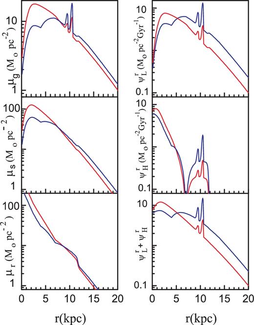
Radial profiles of densities and star formation rates disturbed by local streams plotted for the present epoch and boundary time τb = 50 Myr. Red lines correspond to a model with constant tf = 2.25 Gyr; blue lines correspond to the IO scenario from Chiappini et al. (2001).
Search for parameters derived for two models of tf (in Gyr) and two boundary times τb. For comparison with results in MT18, we give the minima of the residual function Δ2 and oxygen masses PO (in solar units) ejected per core-collapse supernova event derived in the present paper and in MT18. The masses of the streams (m1, 2) are given in 108 M⊙.
Search for parameters derived for two models of tf (in Gyr) and two boundary times τb. For comparison with results in MT18, we give the minima of the residual function Δ2 and oxygen masses PO (in solar units) ejected per core-collapse supernova event derived in the present paper and in MT18. The masses of the streams (m1, 2) are given in 108 M⊙.
In Fig. 3 we plot our results for the radial oxygen distributions, obtained using the perturbed model for the Galactic oxygen evolution; the theoretical distributions are superimposed on the observed binned distribution. The derived parameters are given in Table 1. As can be seen, the effect of local low-abundant streams, which infall on to the disc during a short period of time at the last epoch, indeed results in a decrease of oxygen abundance at the stream locations.
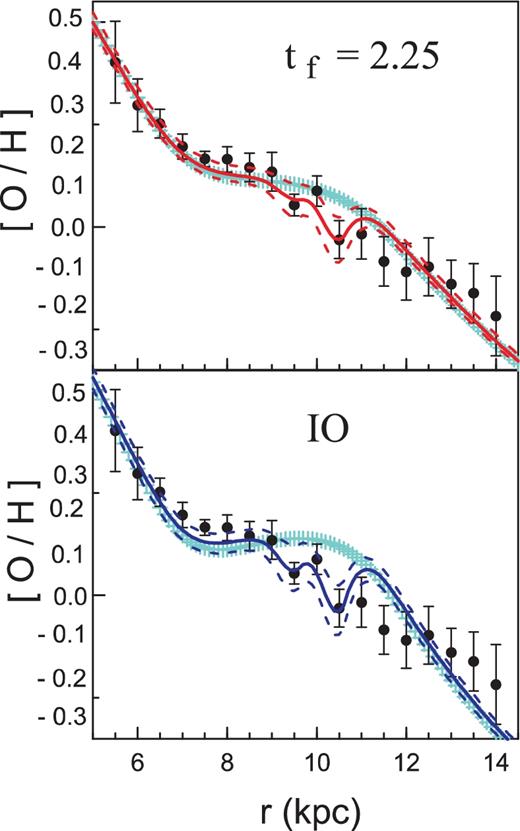
The theoretical oxygen distributions for the present epoch superimposed on the observed binned pattern from Fig. 1; the theoretical local dips follow the observed ones well. Upper panel: the theoretical pattern computed for the time-scale of unperturbed gas infall tf = 2.25 Gyr. Bottom panel: as above, but for the IO scenario of Chiappini et al. (2001). Solid lines represent the best solutions; dashed lines indicate the standard deviations from the best solutions. Cyan lines correspond to the models of oxygen patterns from MT18.
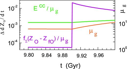
Contributions |$\Delta \dot{Z}_{\rm O}$| to |$\dot{Z}_{\rm O}$| from exploding core-collapse supernova events (green line) and the dilution of oxygen abundance by the infall low-abundant gas (magenta line), including perturbations by the stream. The contributions were computed at r = 10.5 kpc. The effects of both processes become apparent for t ≥ 9.9 Gyr (for details, see equation 10).
As can be seen from Fig. 4, if t < 9.9 Gyr the unperturbed rate of Galactic disc enrichment by oxygen owing to CC SN explosions (green line) exceeds the effect of oxygen dilution by the gas infall (magenta line). But as soon as the (transient) stream begins to interact with the Galactic disc, the dilution of the ISG by low-density gas in the stream rises sharply at the time t ∼ 9.9 Gyr, but the enrichment rate at the same time does not demonstrate such a rapid growth. The slow growth of the enrichment rate (relative to the dilution) is associated both with the slow growth of μg with time after the stream begins to fall on to the disc (see Fig. 4) and with the weak dependence of the term Ecc/μg on the gas density: |$E^{\rm cc}/\mu _{\rm g}\propto \mu _{\rm g}^{\rm 0.5}$| (see equation 4). In contrast, being a function of fΣ, the dilution rate sharply increases (by about two orders of magnitude) at t = 9.9 Gyr as a result of the significant increase in the infall rate owing to the streams (fΣ = f → f + fst), although the dilution rate depends on the gas density as |$\mu _{\rm g}^{\rm -1}$|. Indeed, at r = 10.5 kpc and t = 9.9 Gyr the numerical value for the regular infall rate is f ∼ 0.13 M⊙ pc-2 Gyr-1 (here we use f0 = 220 M⊙ pc-2 Gyr-1 from MT18), whereas the perturbation in infall rate owing to the stream can be estimated as |$f_{\rm st}\sim m_2/(2\pi r_2 2d_2\delta t)\sim 30$| M⊙ pc−2 Gyr−1, which is much larger than the regular f.
We now comment on the other parameters given in Table 1. First of all, we note that local streams have led to a significant decrease of the minimal values for the residual function Δ2 with respect to the case in which we neglected the perturbations: about 1.8 times for constant tf = 2.25 Gyr and 2.7 times for the IO scenario. In other words, the models with streams satisfy observations much better than those in which the effects of the streams were omitted. This inference can be seen by eye in Fig. 3, where for comparison we plot oxygen distributions (cyan lines) from MT18.
The masses in the streams, required to explain the observed local dips in oxygen radial pattern, are reasonable. For instance, according to table 1 from D'Onghia & Fox (2016), the total mass in the Magellanic Stream and Bridge is ∼4.5 × 10⁸ M⊙ and ∼109 M⊙ in the form of neutral and ionized hydrogen, respectively. Our total masses, needed for explanation of the two local dips (∼2 × 10⁸ and ∼5 × 10⁸ M⊙ for tf = 2.25 Gyr and IO scenario, respectively, see Table 1 in the present paper), are smaller than the total mass of the Magellanic Stream and Bridge.
In Fig. 3, there is a feature in the distance range 11–12.5 kpc that could be interpreted as a third dip. It is possible, however, that there is a rise in the oxygen abundance in the range 12.5–14 kpc associated with the outer Lindblad resonance located at r ∼ 12 kpc. Therefore, the nature of this feature is not as unambiguous as the nature of the previous dips. This feature will be studied separately.
4 CONCLUSIONS
The binned oxygen distribution along the Galactic radius, constructed using oxygen abundances in Cepheids from 4KMLL, demonstrates at least two features: a multi-slope radial gradient with a plateau-like distribution within the region 7 ≲ r ≲ 9 kpc, and local dips at r ∼ 9.5 and 10.5 kpc (Fig. 1). The first feature was explained in MT18 by means of the combined effect of the corotation resonance (located at r ∼ 7 kpc) and turbulent diffusion.
In the present paper, we associate the formation of the local dips in oxygen abundance at the aforementioned distances with the local transient intergalactic low-density gas infall (the streams) on to the Galactic disc. As can be seen from Fig. 3, if we incorporate the above local streams in the model for oxygen Galactic synthesis, proposed by MT18, we explain both the nature of the large-scale radial oxygen distribution along the disc (with the plateau-like feature) and the local dips. The total mass for the streams is 2–5 × 10⁸ M⊙, which is comparable to the observed values (cf. D'Onghia & Fox 2016).
The mean mass of oxygen, PO, ejected per CC SN event, and the upper initial masses of stars, mU, which explode as CC SNe and contribute to the disc enrichment by oxygen, are close to the values derived in MT18.
ACKNOWLEDGEMENTS
The authors thank Dr M. Mollá for a scrupulous reading of the manuscript and many important remarks and suggestions which improved our paper.
Footnotes
Unfortunately, we have noticed a typo in the corresponding equation (8) of MT18: the inequality symbols were written incorrectly. The correct ratios between τm and τb for long- and short-lived stars are given in equation (2) of the present paper. For computer calculations in MT18, however, we used the correct ratios for the stellar lifetime and the boundary time.
Recall that the Galactic disc rotates differentially (Ω is a function of the Galactocentric distance r), whereas spiral waves rotate as a rigid body (ΩP = const), the distance rc at which the two velocities are equal (Ω(rc) = ΩP) is termed the corotation resonance; in our case, rc ∼ 7 kpc and the bend in Fig. 1 is located close to the corotation resonance.
In order to derive equations that describe the chemical evolution of the Galactic disc in the framework of separate SFRs for low- and high-mass stars, it is convenient to use SFRs defined by numbers. However, in order to compare radial profiles for SFRs with the ones published in literature we introduce the reduced SFRs determined by ‘mass’: |$\psi ^{\rm r}_{\rm L} = \psi _{\rm L}\int _{0.01}^{m_{\rm b}}m\xi {\rm d}m$| and |$\psi ^{\rm r}_{\rm H}=\psi _{\rm H}\int _{m_{\rm b}}^{m_{\rm U}}m\xi {\rm d}m$|, the units for the reduced SFRs being M⊙ pc-2 Gyr-1.
REFERENCES
