


Abstract
Large sky surveys are increasingly relying on image subtraction pipelines for real-time (and archival) transient detection. In this process one has to contend with varying point-spread function (PSF) and small brightness variations in many sources, as well as artefacts resulting from saturated stars and, in general, matching errors. Very often the differencing is done with a reference image that is deeper than individual images and the attendant difference in noise characteristics can also lead to artefacts. We present here a deep-learning approach to transient detection that encapsulates all the steps of a traditional image-subtraction pipeline – image registration, background subtraction, noise removal, PSF matching and subtraction – in a single real-time convolutional network. Once trained, the method works lightening-fast and, given that it performs multiple steps in one go, the time saved and false positives eliminated for multi-CCD surveys like Zwicky Transient Facility and Large Synoptic Survey Telescope will be immense, as millions of subtractions will be needed per night.
1 INTRODUCTION
Time-domain studies in optical astronomy have grown rapidly over the last decade with surveys like All Sky Automated Survey for Supernovae (ASAS-SN) (Pojmański 2014), Catalina Realtime Transient Survey (CRTS) (Mahabal et al. 2011; Djorgovski et al. 2011; Drake et al. 2009), Gaia (Gaia Collaboration et al. 2016), Palomar-Quest (Djorgovski et al. 2008), Panchromatic Survey Telescope and Rapid Response System (Chambers et al. 2016) and Palomar Transient Factory (PTF) (Law et al. 2009), to name a few. With bigger surveys like Zwicky Transient Facility (ZTF) (Bellm 2014) and Large Synoptic Survey Telescope (LSST) (Ivezic et al. 2008) around the corner, there is even more interest in the field. Besides making available vast sets of objects at different cadences for archival studies, these surveys, combined with fast processing and rapid follow-up capabilities, have opened the doors to an improved understanding of sources that brighten and fade rapidly. The real-time identification of such sources – called transients – is, in fact, one of the main motivations of such surveys. Examples of transients include extragalactic sources such as supernovae and flaring M-dwarf stars within our own Galaxy, to name just two types. The main hurdle is identifying all such varying sources quickly (completeness) and without artefacts (contamination). The identification process is typically done by comparing the latest image (hereafter called the science image) with an older image of the same area of the sky (hereafter called the reference image). The reference image is often deeper, so that fainter sources are not mistaken as transients in the science image. Some surveys like CRTS convert the images to a catalogue of objects using source extraction software (Bertin & Arnouts 1996) and use the catalogues as their discovery domain, comparing the brightness of objects detected in the science and reference images. Other surveys like PTF difference the reference and science images directly after proper scaling and look for transients in the difference images.
The reference and science images differ in many ways. (1) Changes in the atmosphere mean the way light scatters is different at different times. This is characterized by the point-spread function (PSF). (2) The brightness of the sky changes depending on the phase and proximity to the Moon. (3) The condition of the sky can be different (e.g. very light cirrus). (4) The noise and depth (detection limit for faintest sources) are typically different for the two images. As a result, image differencing is non-trivial and along with real transients come a large number of artefacts per transient. Eliminating these artefacts has been a bottleneck for past surveys, with humans having often been employed to remove them one by one – a process called scanning – in order to shortlist a set of genuine objects for follow-up using the scarce resources available. Here we present an algorithm based on deep learning that eliminates artefacts almost completely and is nearly complete (or can be made so) in terms of the real objects that it finds. In Section 2 we describe prior work for image differencing and on deep learning in astronomy. In Section 3 we describe the image differencing problem in greater detail, in Section 4 we present our method and a generative encoder–decoder network – called TransiNet hereafter – based on convolutional networks (hereafter ConvNets or CNNs), in Section 5 we detail the experiments we have carried out and in Section 6 we discuss future directions.
2 RELATED WORK
For image differencing, some of the programs that have been used include those of Alard & Lupton (1998), Bramich (2008), and ptfide (Masci et al. 2017). A recent addition to the list is zogy (Zackay, Ofek & Gal-Yam 2016), which apparently has lower contamination by more than an order of magnitude. It is to be used with the ZTF pipeline and at least in parts of the LSST pipeline. The main task of such an algorithm is to identify new point sources (convolved with the PSF). The problem continues to be challenging because it has to take many complicating factors into consideration. Besides maximizing real sources found (true positives), generating as clean an image as possible (fewest false positives) is the quantifiable goal. Please refer to Zackay et al. (2016) for greater detail.
Neural networks in their traditional form have been around since as early as the 1980s (e.g. LeCun 1985; Rumelhart & Hinton 1986). Such classical architectures have been used in astronomical applications in the past. One famous example is the star–galaxy classifier embedded into the SExtractor package (Bertin & Arnouts 1996).
The advent of convolutional neural networks (ConvNets: LeCun et al. (1990, 1998)), followed by advances in parallel computing hardware (Raina, Madhavan & Ng 2009), has started a new era in ‘deep’ convolutional networks, specifically in the areas of image processing and computer vision. The applications span from pixel-level tasks such as denoising to higher-level tasks such as detection and recognition of multiple objects in a frame (see e.g. Krizhevsky, Sutskever & Hinton 2012; Simonyan & Zisserman 2014).
Researchers in the area of astrophysics have also very recently started to utilize deep learning-based methods to tackle astronomical problems. Deep learning has already been used for galaxy classification (Hoyle 2016), supernova classification (Cabrera-Vives et al. 2017), light-curve classification (Charnock & Moss 2017; Mahabal et al. 2017), identifying bars in galaxies (Abraham et al. 2017), separating near-Earth asteroids from artefacts in images (Brian Bue, private communication), transient-selection post-image differencing (Morii et al. 2016), gravitational wave transient classification (Mukund et al. 2017) and even classifying noise characteristics (Abbott 2017; George, Shen & Huerta 2017; Zevin 2017).
One aspect of ConvNets that has not received enough attention in the astrophysical research community is the ability to generate images as output (Rezende, Mohamed & Wierstra 2014; Bengio et al. 2013). Here, we provide such a generative model to tackle the problem of contamination in difference images (see Fig. 1) and thereby simplify the transient follow-up process.
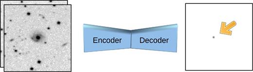
Our CNN-based encoder–decoder network, TransiNet, produces a difference image without an actual subtraction. It does so through training, using a labelled set of transients as the ground truth.
3 PROBLEM FORMULATION
We cast the transient-detection problem as an image-generation task. In this approach, the input is composed of a pair of images (generally with different depth and seeing, aka full width at half-maximum (FWHM) of the PSF) and the output is an image containing, ideally, only the transient at its correct location and with a proper estimation of the difference in magnitudes. In this work, we define a transient as a point source appearing in the second/science input image and not present in the first/reference image. A generative solution such as we propose naturally has at its heart registration, noise-removal, sky subtraction and PSF matching.
In computer vision literature, this resembles a segmentation task, where one assigns a label to each pixel of an image, e.g. transient versus non-transient. However, our detections include information about the magnitude of the transients and the PSF they are convolved with, in addition to their shape and location. Therefore the pixels of the output are real-valued (or are in the same space as the inputs), making the problem different from simple segmentation (see Fig. 2). To this end, we introduce an approach that is based on deep learning and train a ConvNet to generate the expected output based on the input image pair.

Examples of the reference (left) and science (centre) images. The image on the right is the ground-truth output defined for this image pair. It contains the image of a single transient, completely devoid of background and noise. The profile of the transient is the best match to reality our model can produce.
It is the ideal model for the transient and can be seen as an empty image with an ideal point source on it. Based on our formulation of the problem, the answer we seek is It*ϕ2, which represents the image containing the transient in the same seeing conditions as the science image. This involves PSF matching, for taking the first image from I0*ϕ1 to I0 and then to I0*ϕ2, for the subtraction to work.
4 METHOD
We tackle the problem using a deep-learning method, in which an encoder–decoder convolutional neural network is responsible for inferring the desired difference image based on the input pair of images.
4.1 Network architecture
We illustrate TransiNet in Fig. 3. Such architectures have traditionally been used to learn useful representations for the input data in the encoder network, by training the encoder and decoder in an end-to-end fashion, forcing the generative network to reconstruct the input – i.e. auto-encoders such as described by Vincent et al. (2008).
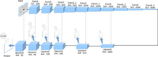
Our suggested fully convolutional encoder–decoder network architecture. The captions at the top/bottom of each layer show the kernel size, followed by the number of feature maps. Each arrow represents a convolution layer with a kernel size of 3 × 3 and stride and padding values of 1, which preserves the spatial dimensions. Dotted lines represent the skip connections. Low-resolution outputs are depicted on top of each up-convolution layer, with the corresponding loss. After each (up-)convolution layer there is a ReLU layer, which is not displayed here.
4.2 Data preparation
Deep neural networks are in general data-greedy and require a large training data set. TransiNet is not an exception and in view of the complexity of the problem – and equivalently the architecture – needs a large number of training samples: reference–science image pairs as well as their corresponding ground-truth images. Real astronomical image pairs with transients are not readily available. The difficulty of providing proper transient annotations makes them even scarcer. The best one can do is to annotate image pairs manually (or semi-automatically) and find smart ways to estimate a close-to-correct ground-truth image: a clean difference image with background-subtracted gradients. Although, as explained in Section 4.2.1, we implement and prepare such a real training set, it is still too small (∼ 200 samples) and, if used as is, the network would easily overfit it.
One solution is to use image-augmentation techniques, such as spatial transformations, to increase the size of the training set virtually. This trick, though necessary, is still not sufficient in our case with only a few hundred data samples – the network eventually discovers common patterns and overfits to the few underlying real scenes.
An alternative solution is to generate a large simulated (aka synthetic) data set. However, relying only on synthetic data makes the network learn features based on the characteristics of the simulated examples, making it difficult to transfer knowledge to the real domain.
Our final solution is to feed the network with both types of data: synthetic samples mixed with real astronomical images of the sky with approximate annotations. This, along with online augmentation, makes a virtually infinite training set, which has the best of both worlds. We describe details of the data sets used and the training strategy in the following subsections.
4.2.1 Real data
For real examples, we make use of data from the Supernova Hunt project (SN Hunt: Howerton 2017) of the CRTS survey. In this project, image subtraction is performed on pairs of images of galaxies in search of supernovae. While this may bias the project towards finding supernovae rather than generic transients, that should not affect the end result, as we mark the transients found and the ground-truth images contain just the transients. If anything, finding such blended point sources should make finding point sources in the field (i.e. away from other sources) easier. Unlike most other surveys, the CRTS images are obtained without a filter, but that too is not something that concerns our method directly. We gathered 214 pairs of publicly available JPEG images from SN Hunt and split this data set into training, validation and test subsets of 102, 26 and 86 members respectively. The reference images are typically made by stacking ∼20 older images of the same area. The science image is a single 30-sec exposure. The pixels are 2.5 × 2.5 arcsec2 and thus comparable to or somewhat bigger than the typical PSF. Individual images are 120 × 120 pixels and at times not perfectly registered.
To prepare the ground truth, we developed an annotation tool. The user needs to define the location of the transient roughly in the science image, by comparing it with the reference image, and to put a circular aperture around it. Then the software models the background and subtracts it from the aperture to provide an estimate of the transient's shape and brightness. Simple annulus-based estimates of the local background (Davis 1987; Howell 1989) or even the recent Aperture Photometry Tool (Laher et al. 2012) are not suitable for most of the samples of this data set, since the transients, often supernovae, naturally overlap their host galaxies. Therefore we use a more complex model and fit a polynomial of degree 8 to a square-shaped neighbourhood of size 2r × 2r around the aperture, where r is the radius of the user-defined aperture. Note, however, that model fitting is performed only after masking out the aperture to exclude the effect of the transient itself – the points are literally excluded from model fitting – rather than the aperture being masked and replaced with a value such as zero. This method works reasonably well even when the local background is complex. Fig. 4 illustrates the process.
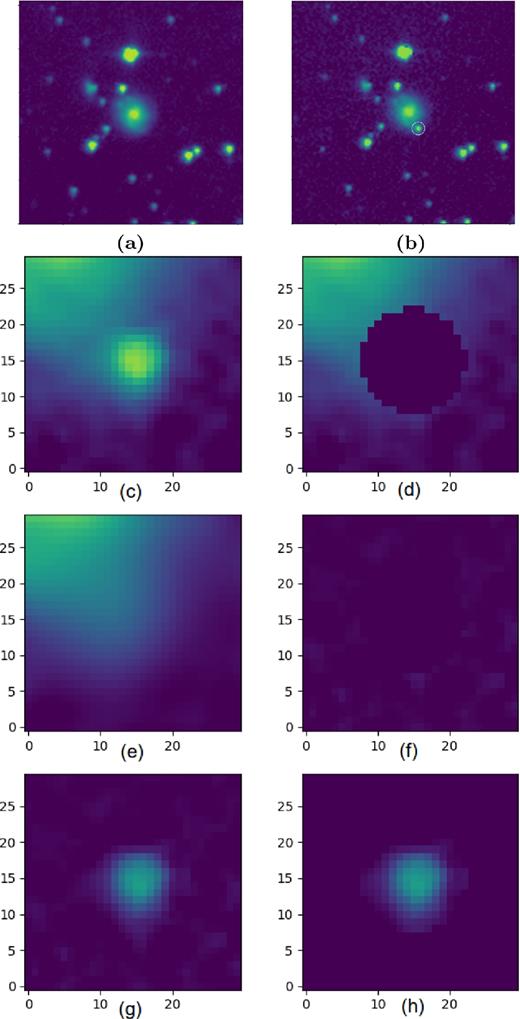
An exemplar transient annotation case: (a) input reference image; (b) input science image; (c) 2r × 2r neighbourhood of the transient; (d) masked-out user-defined aperture; (e) polynomial model fitted to the ‘masked neighbourhood’ (note that, since the blank aperture is excluded from the fitting process, there is no dark region in the results); (f) estimated background subtracted from the masked neighbourhood to form a measure of how well the background has been modelled (the more uniform and dark this image is, the better the polynomial has modelled the background); (g) the estimated background subtracted from the neighbourhood with the transient standing out; (h) the transient cropped out of (g) using the user-defined aperture.
The annotations on real images are not required to be accurate, as the main responsibility of this data set is to provide the network with real examples of the sky. This lack of accuracy is compensated for by synthetic samples with precise positions.
4.2.2 Synthetic data
To make close-to-real synthetic training samples, we need realistic background images. Existing simulators, such as Skymaker (Bertin 2009), do not yet provide a diverse set of galaxy morphologies and therefore are not suitable for our purpose. Instead, we use images from the Kaggle Galaxy Zoo data set,1 based on the Galaxy Zoo 2 data set (Willett et al. 2013), for our simulations. To this end, we pick a single image as the background image and create a pair of reference–science images based on it.
This method also makes us independent of precise physical simulation of the background, allowing us to focus on simulations only at the image level – even for the ‘foreground’, i.e. transients. This may result in some samples that do not resemble a ‘normal’ astronomical scene exactly, in terms of the magnitude and location of the transient or the final blur of the objects. However, that is even better in a learning-based method, as the network will be trained on a more general set of samples and less prone to overfitting to specific types of scenes. Fig. 5 illustrates the details of this process.
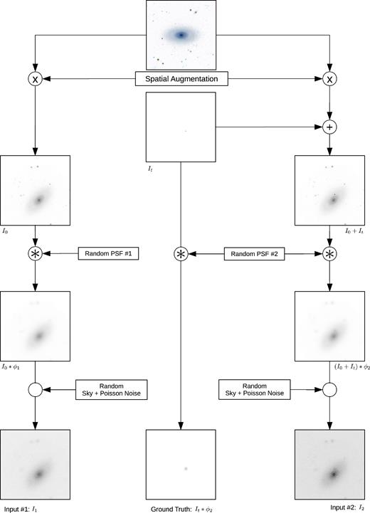
The synthetic sample generation procedure. The notations used here are described in equations (1) and (2).
Modelling the difference between reference and science images precisely and adjusting the PSF parameter distributions accordingly would be achievable. However, as stated before, we prefer to keep the training samples as general as possible. Therefore, in our experiments [σϕ, m, σϕ, M] is set to [2,5] for both images. These numbers are larger than typically encountered and real images should fare better. The eccmax value is set to 0.4 and 0.6 for reference and science images, respectively, to model the more isotropically blurred seeing of reference images.
Then we perform a pairwise augmentation (rotation, scaling and translation), such that the two images are not perfectly registered. This forces the network also to learn the task of registration on the fly.
The ground-truth image is then formed by convolving the ideal transient image, It, with the same PSF as applied to the science image. No constant sky value or noise are applied to this image. This way, the network learns to predict transient locations and their magnitudes in the same seeing conditions as the science image, in addition to noise removal and sky subtraction.
4.3 Training details
We train two versions of the network. The first one is trained solely on synthetic data, while the other uses both synthetic and real data. To this end, we initially train both networks for 90K iterations, on synthetic images of size 140 × 140, grouped in batches of size 16. Then, in the second network only, we continue training on a mixture of real and synthetic data of size 256 × 256 for another 8K iterations. We put 12 real images and four synthetic images in each batch during this second round of training to prevent overfitting to the small-sized (∼100) real SN Hunt samples.
We use ADAM for optimization using the Caffe framework (Jia et al. 2014). We start with a learning rate of 3e−4 and drop it in the second round by a factor of 0.3 every 20K iterations. On an NVIDIA GTX 1070 along with 16 CPU cores, the whole training process takes a day and half to complete.
The attention trick
In this specific type of application, the target images consist mainly of black regions (i.e. zero-intensity pixels), with non-zero regions taking only a small number of pixels. Therefore mere use of a simple L1 loss does not generate and propagate large enough error values back to the network, especially when the network has just learned to remove the noise and generates blank images. The network therefore spends too long a time focusing on generating blank images instead of the desired output and in some cases fails to even converge. The trick we use to get around this issue is to boost the error in the interesting regions conditionally. The realization of this idea is simply to apply the mapping [0, 1] → [0, K] on the ground-truth pixel values. K represents the boosting factor and we set it to 100 in our experiments. This effectively boosts the error in non-zero regions of the target, virtually increasing the learning rate for those regions only. The output of the network is later downscaled to lie in the normal range. Note that increasing the total learning rate is not an alternative solution, as the network would go unstable and would not even converge.
5 EXPERIMENTS AND RESULTS
We now have two versions of TransiNet at hand: one trained only with synthetic data based on the Kaggle Zoo and another fine-tuned on samples from the real CRTS SN Hunt data set. The former is the experimental, but more flexible network, in which one can evaluate the performance of the network while varying different parameters of the input/transients. However, the latter is the one showing the performance of TransiNet in a real scenario. In theory, four groups of experiments can be reported, based on two trained models, (a) synthetic and (b) synthetic+real, and two different test sets, (a) synthetic and (b) real. However, training on the synthetic+real model and testing on synthetic only does not make much sense and has been left out. The three experiments we report on are as follows: (a) Synthetic: training on synthetic data, testing on synthetic data; (b) Transfer: training on synthetic, testing on real; (c) Real or CRTS: training on synthetic+real, testing on real. We report the results of the Transfer experiment just to show the necessity for a small real training subset.
The network weights take up about 2 GB of memory. Once read, on the NVIDIA GTX 1070 the code runs fast: 39 ms per sample, which can be reduced to 14 ms if samples are passed to the network as batches of 10. The numbers were calculated by running tests on 10 000 images three times.
Fig. 6 depicts samples from running TransiNet on the CRTS test subset – the ‘Real’ experiment. The advantage of TransiNet is that the ‘image differencing’ produces a noiseless image which, with the correct threshold, ideally consists of just the transient. It is robust to artefacts and removes the need for human scanners. At the same time, by tweaking the threshold one can choose to optimize precision or recall based on one's needs.
![Image subtraction examples using ZOGY and TransiNet for a set of CRTS Supernova Hunt images. The first column has the deep reference images; the second column contains the science images, which have a transient source and are a shallower version of the reference images. The third column contains the ZOGY D images and the fourth has the ZOGY Scorr images, i.e. ‘the matched filter difference image corrected for source noise and astrometric noise’ (Zackay et al. 2016). The fifth column has the thresholded versions of ZOGY SCORR, as recommended in that article. The sixth column shows the difference image obtained using TransiNet. All images are mapped to the [0,1] range of pixel values, with a gamma correction on the last column for illustration purposes. TransiNet has a better detection accuracy and is also robust against noise and artefacts. It is possible that ZOGY could be tuned to perform better and, on a different data set, provide superior results – the reason for the comparison here is simply to show that TransiNet does very well.](https://oup.silverchair-cdn.com/oup/backfile/Content_public/Journal/mnras/476/4/10.1093_mnras_sty613/1/m_sty613fig6.jpeg?Expires=1750216685&Signature=0AXNL3y2SmGTzBEqnqP9xpp3ohxXS-G6TbfMxBQg51CSopkLL~WI3Gwv2Y3Rdd2TKZ8TLvfIyNmcRwVX5T64J8dkBKIFsgXMVy0YlB4WZh7izol3cWeecG3Vf0f3Y-Ts6TDMBZCy~TJv~~7pKFqdBa8iDLlrQR4nvG8StSF~IHBMyoJjatBt4ijGWDSnAcUHmK-VQOEpBSfjNeSBFYIDbjQxprHrmsCzin4skeitfnXMEE4WW1uUxte3K8lFKm6kD1vuYJLpMeLkpj6mJghLIzGVDbMCCrdFcRNEe883V8Ei05hHvuxsv24GmxHsvQiFuRegE0yxWP4USNRSk9E5SA__&Key-Pair-Id=APKAIE5G5CRDK6RD3PGA)
Image subtraction examples using ZOGY and TransiNet for a set of CRTS Supernova Hunt images. The first column has the deep reference images; the second column contains the science images, which have a transient source and are a shallower version of the reference images. The third column contains the ZOGY D images and the fourth has the ZOGY Scorr images, i.e. ‘the matched filter difference image corrected for source noise and astrometric noise’ (Zackay et al. 2016). The fifth column has the thresholded versions of ZOGY SCORR, as recommended in that article. The sixth column shows the difference image obtained using TransiNet. All images are mapped to the [0,1] range of pixel values, with a gamma correction on the last column for illustration purposes. TransiNet has a better detection accuracy and is also robust against noise and artefacts. It is possible that ZOGY could be tuned to perform better and, on a different data set, provide superior results – the reason for the comparison here is simply to show that TransiNet does very well.
With increasing CCD size it is much more likely than not that there will be multiple transients in a single image. Since the SN Hunt images and the zoo images used rarely have multiple transients, the networks may not be ideal when looking for such cases. However, because of the way the network is trained – with the output as pure PSF-like transients – it is capable of finding multiple transients. This is demonstrated in Fig. 7, which depicts an exemplar sample from the zoo subset. Here we introduced four transients and all were correctly located. Another positive side effect is that the network rejects non-PSF-like additions, including cosmic rays. In addition to the four transients, we had also inserted 10 single-pixel cosmic rays into the science image shown in Fig. 7 and all were rejected. An example from the SN Hunt set is shown in Fig. 8, which happens to have two astrophysical objects – the second is likely an asteroid. Here too the network has detected both transients. Locating new asteroids is as useful as locating transients to help make the asteroid catalogue more complete for future linking and position prediction.
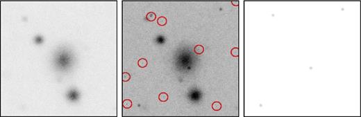
An exemplar multi-transient case from the zoo data set: the reference image (left), science image (middle) with 10 single-pixel Cosmic Ray events, indicated by red circles, and four transients and the network prediction (right) with all transients detected cleanly and all CRs rejected.
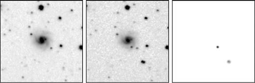
An exemplar multi-transient case from the CRTS SN Hunt data set. The science image (middle) has two transients and the network prediction (right) finds them both, though it was never trained explicitly to look for multiple transients.
5.1 Quantitative evaluation
We provide below quantitative evaluations of TransiNet performance.
5.1.1 Precision-recall curve
Low-SNR detections and blank outputs
The output of TransiNet is an image with real-valued pixels. Therefore each pixel is more likely to contain a non-zero real value, even in the ‘dark’ regions of the image or when there is no transient to detect at all. Thus, we consider low signal-to-noise ratio (SNR) detection images as blank images. The outputs of the network (detection images) that have a standard deviation (σ) lower than 0.001 were marked as blank images during our experiments and not considered thereafter.
Binarization and counting of objects
Evaluation at a series of thresholds is the essence of a precision-recall curve and helps reveal low SNR contaminants, while digging for higher completeness (see Fig. 9).
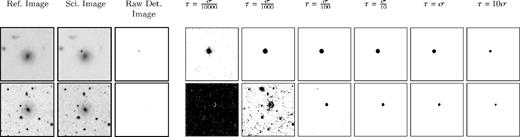
Visualization of the thresholding process used for generation of precision-recall curves. Each row illustrates exemplar levels of thresholding of a single detection image: the first row is chosen from the synthetic subset and the second row from CRTS. Outputs of the network are normally quite clean and contaminants appear only after taking the threshold down below the noise level. This is particularly visible in the second row, where the transient has been of a low magnitude and so the detection image has a low standard deviation (σ). Thus σ/100 is still too low and below the noise level.
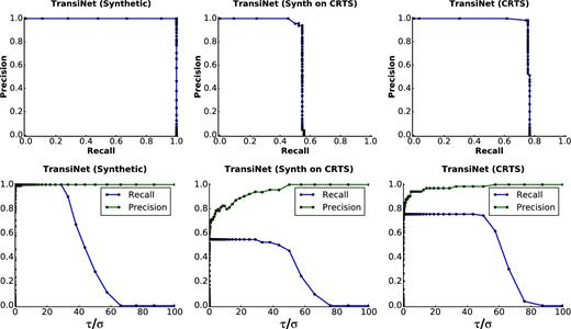
Plots showing precision-recall curves (top row) and their dependence on the threshold (bottom row) for TransiNet. The column on the left shows the Synthetic experiment, in which the train and test sets are both taken from synthetic data. In the middle column we depict the performance drop in the experiment in which the network is trained only on synthetic data, but is tested on real data. In the right column (CRTS), we leverage the real training subset to boost the performance on real data. Not unexpectedly, the performance is close to ideal for the synthetic images. For CRTS, we never go above a recall (completeness) of 80 per cent, but all those detections are clean and the ones we miss are the really low significance ones below the threshold of 0.001. Thus a threshold can be picked where 80 per cent of transients are detected with high precision (little contamination).
The sharp and irregular behaviour of the curve at around 75 per cent recall in the CRTS experiment is due to the low contamination levels in the output: transients are detected with a high significance. Contaminants, if any, have a much lower intensity and their number goes up only when one pushes for high completeness to lower significance levels. Similar behaviour can be seen in the other two experiments also. This allows one to choose a fixed threshold in this region of the curve for the final deployed detector based on requirements.
5.1.2 Relative magnitude of the transient
Thanks to the freedom inherent in generation of synthetic samples with different parameters, we can evaluate the performance of the network with transients of different magnitudes. However, for this evaluation we use relative magnitudes, as opposed to the absolute intensities used during training. This would make it easier to determine quantitatively the ability of the network to detect faint transients without contamination. In the future, we hope to incorporate similar process during training as well.
Fig. 11 depicts the performance of the detector for several relative magnitudes, in terms of the precision-recall curve. With higher visibility, the curve approaches the ideal form. Considering that, during the training phase, the network has rarely seen transients with such low magnitudes as the ones in the lower region of this experiment, it is still performing well. We expect it to gain much better results by broadening the range of simulated transient amplitudes during training.
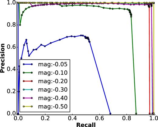
Precision-recall curves for a range of magnitudes. These are for the synthetic transients, where we had control over the relative magnitudes. The network misses more transients as the relative magnitude goes lower. This is not unexpected, as the network has not seen such faint samples during training. The sharp vertical transitions reflect the clean nature of the detection images.
5.1.3 Robustness to spatial displacements
We analyse the robustness of TransiNet to pairwise spatial inconsistencies between the science and reference images. That way small rotations, World Coordinate System (WCS) inconsistencies, etc., do not give rise to yin–yang like ‘features’ and lead to artefacts. To this end, for a subset of image pairs, we exert manual shift, rotation and scaling on one of the images in each pair and pass them through the network. Fig. 12 depicts the results of these experiments as plots of completeness and contamination versus manual perturbation.
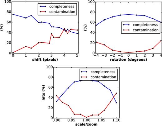
Robustness of the network to shift (top left), rotation (top right) and scaling (bottom) between the reference and science images for CRTS. Ideally there will be no misalignments, but some can creep in through improper WCS, changes between runs, etc.
5.1.4 Numerical performance of TransiNet
Table 1 summarizes the testing results for the TransiNet networks, with chosen fixed thresholds. For new surveys, one can start with the generic network and, as events become available, fine-tune the network with specific data.
Hits and misses for TransiNet for the synthetic and SN Hunt networks. TransiNet does very well for synthetics. One reason could be that there is not enough depth variation in the reference and science images. However, for CRTS too the output is very clean for the recall of 76 per cent that it achieves. The lower (than perfect) recall could be due to a smaller sample, larger pixels, large shifts in some of the cutouts, etc. Fine-tuning with more data can improve performance further. The fixed threshold used in the first two rows was 20, while it was set to 40 for the last row, consistent with Fig. 10.
| Network | Tran | TP | FP | FN | Prec. | Recall |
|---|---|---|---|---|---|---|
| Synthetic | 100 | 100 | 0 | 0 | 100.0 | 100.0 |
| Transfer | 86 | 47 | 6 | 39 | 88.7 | 54.6 |
| CRTS | 86 | 65 | 1 | 21 | 98.4 | 75.5 |
| Network | Tran | TP | FP | FN | Prec. | Recall |
|---|---|---|---|---|---|---|
| Synthetic | 100 | 100 | 0 | 0 | 100.0 | 100.0 |
| Transfer | 86 | 47 | 6 | 39 | 88.7 | 54.6 |
| CRTS | 86 | 65 | 1 | 21 | 98.4 | 75.5 |
5.2 Comparison with ZOGY
Given the generative, and hence very different, nature of our ‘pipeline’, it is difficult to compare it with direct image differencing pipelines. We have done our best by comparing the output of TransiNet and ZOGY for synthetic as well as real images. We used the publicly available matlab version of ZOGY and almost certainly used ZOGY in a sub-optimal fashion. As a result, this comparison should be taken only as suggestive. More direct comparisons with real data (PTF and ZTF) are planned for the near-future. Fig. 6 depicts the comparison for a few of the SN Hunt transients.
Both pipelines could be run in parallel to choose an ideal set of transients, since the overhead of TransiNet is minuscule.
6 FUTURE DIRECTIONS
We have shown how transients can be detected effectively using TransiNet. In using the two networks we described, one with Kaggle Zoo images and another with CRTS, we cover all broad aspects required and yet for this method to work with any specific project, e.g. ZTF, appropriate tweaks will be needed, in particular labelled examples from image differencing generated by that survey. Also, the assumptions during simulations can be improved upon by such examples. Using labelled sets from surveys accessible to us is definitely the next step. Since the method works on the large pixels that CRTS has, we are confident that such experiments will improve the performance of TransiNet.
The current version produces convolved transients to match the shape and PSF of the science image. One can modify the network to produce just the transient location and leave the determination of other properties to the original science and reference images, as they contain more quantitative detail.
Further, the network could be tweaked to find variable sources too. However, for that a much better labelled non-binary training set will be needed. In the same manner, it can also be trained to look for drop-outs, objects that have vanished in recent science images but were present in the corresponding reference images. This is in fact an inverse of the transients problem and somewhat easier to perform.
In terms of reducing the number of contaminants even further, one can provide as input not just the pair of science and reference images but also pairs of the rotated (by 90°, 180°, 270°) and flipped (about the x- and y-axes) versions. The expectation is that the transient will still be detected (perhaps with a slightly different peak extent), but the weak contaminants, at least those that were possibly conjured by the weights inside the network, will be gone (perhaps replaced by other – similarly weak – ones at a different location) and the averaging of detections from the set will leave just the real transient.
Another way to eliminate inhomogeneities in network weights is to test the system with image pairs without any transients. While most image pairs do not have any transient except in a small number of pixels, such a test can help streamline the network better.
In order to detect multiple transients, one could cut the image into smaller parts and provide these subimages for detection. Another possibility is to mask the ‘best’ transient and rerun the pipeline to look for more transients iteratively until none is left. An easier fix is to train the network for larger images and for multiple transients in each image pair.
Another way to improve the speed of the network is to experiment with the architecture and, if possible, obtain a more lightweight network with a smaller footprint that performs equally well. Finally, the current network used JPEGs with limited dynamic range as inputs. Using non-lossy FITS images should improve the performance of the network.
7 CONCLUSIONS
We have introduced a generative method based on convolutional neural networks for image subtraction to detect transients. It is superior to other methods, as it has a higher completeness at lower thresholds and at the same time has fewer contaminants. Once the training is carried out with appropriate labelled data sets, execution on individual images is fast. It can operate on images of any size (after appropriate training) and can easily be incorporated into real-time pipelines. While we have not tested the method explicitly on high-density fields (e.g. closer to the plane of the Galaxy), it will be possible to obtain good performance once a corresponding labelled data set is used for training. We hope that surveys like ZTF and LSST, as well as those with larger pixels like ASAS-SN (Shappee et al. 2014) and Evryscope (Law et al. 2015), will adapt and adopt the method. It is also possible to extend the method to other wavelengths like radio and use it for surveys including Square Kilometer Array and its pathfinders.
ACKNOWLEDGEMENTS
AM was supported in part by the NSF grants AST-0909182, AST-1313422, AST-1413600 and AST-1518308, and by the Ajax Foundation.
Footnotes
REFERENCES
