


Abstract
Supermassive black hole binaries (SMBHBs) should be common in galactic nuclei as a result of frequent galaxy mergers. Recently, a large sample of sub-parsec SMBHB candidates was identified as bright periodically variable quasars in optical surveys. If the observed periodicity corresponds to the redshifted binary orbital period, the inferred orbital velocities are relativistic (v/c ≈ 0.1). The optical and ultraviolet (UV) luminosities are expected to arise from gas bound to the individual BHs, and would be modulated by the relativistic Doppler effect. The optical and UV light curves should vary in tandem with relative amplitudes which depend on the respective spectral slopes. We constructed a control sample of 42 quasars with aperiodic variability, to test whether this Doppler colour signature can be distinguished from intrinsic chromatic variability. We found that the Doppler signature can arise by chance in ∼20 per cent (∼37 per cent) of quasars in the nUV (fUV) band. These probabilities reflect the limited quality of the control sample and represent upper limits on how frequently quasars mimic the Doppler brightness+colour variations. We performed separate tests on the periodic quasar candidates, and found that for the majority, the Doppler boost hypothesis requires an unusually steep UV spectrum or an unexpectedly large BH mass and orbital velocity. We conclude that at most approximately one-third of these periodic candidates can harbor Doppler-modulated SMBHBs.
1 INTRODUCTION
It is well established that most, if not all, massive galaxies harbor supermassive black holes (SMBHs) in their nuclei. The mass of the central BH is correlated with several properties of the host galaxy (e.g. velocity dispersion, bulge luminosity, etc.), which suggests that the SMBH and the host galaxy may co-evolve (Kormendy & Ho 2013). In the hierarchical structure formation model, galaxies and quasars are built up from smaller progenitors through frequent mergers (Haehnelt & Kauffmann 2002). These mergers should result in an SMBHB at the centre of the newly formed galaxy, surrounded by significant amounts of gas (Barnes & Hernquist 1992).
In the post-merger galaxy, the orbit of the binary shrinks initially due to dynamical friction and subsequently by scattering nearby stars (Begelman, Blandford & Rees 1980). At small (sub-pc) separations, three-body interactions become less efficient, and the binaries may stall for a significant fraction of the Hubble time (see e.g. Colpi 2014). In this regime, the ambient gas, which is expected to settle into a circumbinary disc (Barnes 2002), may dominate the binary's orbital decay (Tang, MacFadyen & Haiman 2017), while, at the same time, it can accrete on to the BHs providing bright electromagnetic emission (e.g. Haiman, Kocsis & Menou 2009). The SMBHB is eventually driven to merger by the emission of low-frequency gravitational waves (GWs), which could be detectable in the future by pulsar timing arrays (PTAs; Manchester & IPTA 2013) and by the space-based interferometer LISA (Amaro-Seoane et al. 2017).
The orbital decay of the binary due to its interaction with the circumbinary disc is expected to be slow (Haiman, Kocsis & Menou 2009; Kocsis, Haiman & Loeb 2012a,b; Rafikov 2013, 2016; Kelley, Blecha & Hernquist 2017) and SMBHBs should spend significant time (≳ 106 yr) at sub-pc separations and thus should be fairly common. Despite their expected abundance, SMBHBs have only been detected at large separations, from several kpc (Komossa et al. 2003; Bianchi et al. 2008; Green et al. 2010; Comerford et al. 2011; Fabbiano et al. 2011; Koss et al. 2011; Fu et al. 2015) down to a few pc (Rodriguez et al. 2006). At sub-pc separations, it is much more difficult to spatially resolve the orbit of the binary (see, however, D'Orazio & Loeb 2017) and one has to rely on the effects of the binary on its environment. Several candidates have been identified from large-velocity offsets in quasar spectra, helical morphology of radio jets, etc. (see e.g. recent reviews by Dotti, Sesana & Decarli 2012; Komossa & Zensus 2016).
SMBHBs can also be naturally identified as quasars with periodic variability. First, in hierarchical structure formation models, quasars are thought to be activated by galaxy mergers (Kauffmann & Haehnelt 2000). Recent observations of interacting galaxies have provided further evidence for excess active galactic nucleus (AGN) activity (Goulding et al. 2017). Many quasars may thus host SMBHBs. Second, numerous hydrodynamical simulations of SMBHBs with circumbinary gas discs have found that such binaries would produce bright quasar-like luminosities, but with the accretion rate modulated periodically at the orbital period of the binary (Artymowicz & Lubow 1996; Hayasaki, Mineshige & Sudou 2007; MacFadyen & Milosavljević 2008; Noble et al. 2012; Roedig et al. 2012; D'Orazio, Haiman & MacFadyen 2013; Farris et al. 2014; Gold et al. 2014). In a binary system, periodic variability can also arise from a precessing jet, as the viewing angle of the jet varies periodically (see e.g. Romero et al. 2000; Kun et al. 2014, 2015).
Recently, a large number of quasars with significant periodicity have emerged, mainly from systematic searches in the photometric data bases of large time-domain optical surveys. Graham et al. (2015a, hereafter G15) identified 111 candidates in a sample of ∼245 000 quasars from the Catalina Real-Time Transient Survey (CRTS). Charisi et al. (2016, hereafter C16) analysed a sample of ∼35 000 quasars from the Palomar Transient Factory (PTF) and identified 33 additional candidates, with typically shorter periods and dimmer magnitudes. Another recent candidate, quasar SDSS J0159+0105, was identified to have two periodic components in its variability with a frequency ratio 1:2 from a smaller sample of ∼350 low-redshift quasars in CRTS (Zheng et al. 2016).1
Identifying periodic variability in quasars is extremely challenging; the optical light curves are typically sparse, with seasonal gaps and relatively short baselines compared to the periods (the identified candidates were typically observed only for a limited number of 2–3 cycles). Additionally, quasars show stochastic variability. The overall stochastic variability is successfully described by a damped random walk (DRW) model (Kelly, Bechtold & Siemiginowska 2009; Kozłowski et al. 2010; MacLeod et al. 2010). However, some recent studies, including the analysis of well-sampled light curves from Kepler, have suggested that the variability of quasars may deviate from the DRW model, especially at high frequencies (Mushotzky et al. 2011; Zu et al. 2013; Graham et al. 2014; Kasliwal, Vogeley & Richards 2015; Simm et al. 2016). Kelly et al. (2014) proposed a more generic model for quasar variability, the continuous-time autoregressive moving average, and showed that the irregular sampling may introduce quasi-periodic features, resulting in variability similar to that identified in the SMBHB candidates.2 As was also pointed out by Vaughan et al. (2016), our incomplete knowledge of quasar variability, in combination with the limited quality of the optical light curves, can lead to false detections of periodicity. This was demonstrated in the case of the quasar PSO J3334.2028+01.4075 (Liu et al. 2015), whose follow-up monitoring failed to show persistent periodicity (Liu et al. 2016). In addition, Sesana et al. (2017) calculated the GW background for the population of SMBHBs implied by the identified periodic binary candidates, and found that it is in tension with the current upper limit derived from PTAs. The tension can be alleviated only if the typical masses and/or the mass ratios in this sample are surprisingly lower than expected; this suggests that many of the candidates cannot be genuine SMBHBs.
It is therefore crucial to explore additional signatures that could support the binary hypothesis for any periodic candidate. Several such studies followed the discovery of the first quasar with periodic variability (PG 1302-102; Graham et al. 2015b), including the search for multiple periodic components in the optical variability, as expected from hydrodynamical simulations (Charisi et al. 2015; D'Orazio et al. 2015a), the analysis of the helical structure in the radio jet of PG 1302-102 (Kun et al. 2015; Mohan et al. 2016), and the detection of periodic variability in the infrared (Jun et al. 2015; D'Orazio & Haiman 2017).
Another proposed signature of SMBHBs is to detect evidence for the relativistic Doppler boost. Assuming that the observed periodicity corresponds to the redshifted orbital period of the binary, we can infer that most of the candidates are at sub-pc separations, orbiting with mildly relativistic velocities (a few per cent of the speed of light). If the optical emission arises in gas bound to the individual BHs, e.g. in mini-discs seen in hydrodynamical simulations (Farris et al. 2014; Ryan & MacFadyen 2017), the luminosity of the brighter mini-disc, typically the circum-secondary disc, will be inevitably Doppler boosted. For near-equal-mass binaries, this Doppler-induced variability is expected to be sub-dominant to hydrodynamically introduced fluctuations (Bowen et al. 2017, 2018; Tang, Haiman & MacFadyen 2018), but for unequal-mass binaries, it could dominate the variability (D'Orazio, Haiman & Schiminovich 2015b).
Therefore, even if the optical luminosity in the mini-discs is constant, the unresolved binary will appear blue-shifted (and brighter, for typical spectral slopes, i.e. αν < 3), when the more luminous BH is moving towards the observer, and vice versa. The relativistic Doppler boost may naturally explain the observed light curves, which show smooth quasi-sinusoidal periodicity. We note that the periodic mass accretion rates found in hydrodynamical simulations listed in the Introduction section are more bursty than sinusoidal, and are expected to produce more bursty light curves.
D'Orazio et al. (2015b) proposed this model to explain the variability of the periodic candidate PG 1302-102. In particular, they found that if PG 1302-102 hosts an unequal mass binary (q ≲ 0.05), orbiting not too far from edge-on (≲30°), the Doppler boost should dominate the variability. The model can successfully fit the observed optical light curve. Additionally, with archival data from the GalaxyEvolutionExplorer (GALEX) and the HubbleSpaceTelescope (HST), they showed that the variability amplitudes in the near-UV (nUV) and far-UV (fUV) bands are AnUV/Aopt ∼ 2.13 and AfUV/Aopt ∼ 2.63, respectively, consistent with the prediction from equation (4).
On the other hand, quasars are known to be variable across the electromagnetic spectrum. The optical and UV luminosities typically change almost simultaneously, with minimal interband time-lags (Cutri et al. 1985; Edelson et al. 1996; Giveon et al. 1999; Sakata et al. 2011). Additionally, several studies have indicated that quasars become ‘bluer-when-brighter’ (i.e. the continuum spectral slope becomes steeper in brighter phases); this implies that the variability is wavelength-dependent, with higher variability amplitudes at shorter wavelengths (Kinney et al. 1991; Paltani & Courvoisier 1994; Vanden Berk et al. 2004; Wilhite et al. 2005; Ruan et al. 2014; Hung et al. 2016). For instance, the variability amplitudes in the UV are significantly larger than at optical wavelengths (Welsh, Wheatley & Neil 2011; Zhu et al. 2016).
The above trends suggest that, in general, quasars can show optical/UV variability that may mimic the multiwavelength variability predicted by the Doppler model (equation 4). In this paper, we construct a control sample of aperiodic quasars, and determine how often the intrinsic multiwavelength variability of quasars in this sample produces by random chance amplitudes consistent with the predictions of the Doppler boost model. Such a test is especially important given that the currently available UV data are typically relatively sparse. More specifically, we analyse optical and UV light curves to determine the ratio of the observed variability amplitudes in the two bands (i.e. the left-hand side of equation 4). Next, we fit the available optical and UV spectra with power laws, and from the inferred spectral indices, we compute the expected UV-to-optical amplitude ratio (i.e. the right-hand side of equation 4). We check whether the above two quantities are consistent within their errors. Additionally, as a separate test, for a subsample of periodic quasars we estimate the UV spectral index required in order for the putative binaries to be Doppler boosted, and compare this to the range of observed UV spectral slopes in the control sample.
This paper is organized as follows. In Section 2, we present the construction of the control sample, as well as the sample of periodic candidates, and describe our data analysis. In Section 3 we show the results of our analysis, followed by a discussion in Section 4. We end with a short summary of our findings and the implications of our results in Section 5.
2 SAMPLE AND METHODS
2.1 Sample
In order to statistically assess the significance of an apparent Doppler signature,4 our null hypothesis is that this signature can arise from intrinsic wavelength-dependent variability of quasars, unrelated to binary black holes. In other words, we test how often the relative amplitudes of optical and UV variability are by chance consistent with the prediction from equation (4). For this purpose, we assembled a control sample of quasars and AGNs that do not exhibit periodic variability, but whose properties (luminosities and redshifts) resemble those of the periodic candidates. In order to perform this Doppler null test, the following data are necessary for each source in the control sample: (1) an optical light curve, (2) a UV light curve, temporally coincident with the optical,5 (3) an optical spectrum, and (4) a UV spectrum. Since the availability of UV spectroscopy is limited, we maximized the sample size, starting from a sample of sources with available UV spectra.6
More specifically, we made use of two HST spectroscopic catalogues, which provide calibrated co-added UV spectra: (A) the Atlas of Recalibrated HST Faint Object Spectrograph (FOS) Spectra of AGN and Quasars (Evans & Koratkar 2004) and (B) the Cosmic Origin Spectrograph (COS) quasar catalogue of fUV spectra, provided by the Hubble Spectroscopic Legacy Archive (HSLA; Peeples et al. 2016).7 The FOS and COS catalogues include spectra from 204 and 564 unique sources, respectively, among which 56 are common in the two catalogues.
From the COS catalogue, we eliminated five sources that we could not cross-correlate in the astronomical data base Simbad8 and two additional sources that were classified as X-ray binaries. We also excluded from both catalogues sources classified as BL Lac Objects, since they are known to have distinct variability properties from quasars; e.g. their variability may not arise in the accretion disc, but in a relativistic jet (Edelson 1992). These sources were also excluded from the searches for periodicity in both G15 and C16. We excluded five additional sources from the COS catalogue, and one source (PG 1302-102) which was included in both catalogues, because they were identified as periodic.
For the remaining sources, we extracted optical spectra from the Sloan Digital Sky Survey (SDSS),9 optical light curves from CRTS,10 and UV light curves from GALEX.11 Since, as mentioned above, light curves and spectra in both bands are necessary for the Doppler test we kept in the sample only the sources that had all the necessary information. We note that GALEX obtained simultaneously photometric measurements with two UV filters (covering the nUV and fUV bands), but the fUV light curves are typically more sparse, because quasars are fainter in fUV. Moreover, the UV spectra usually do not extend to both bands. So if, for instance, the UV spectrum covers only the fUV band, we checked only for the availability of the fUV light curve (with the additional requirement mentioned before, i.e. two distinct epochs and temporal coincidence with the optical data). We note that this step dramatically decreases the sample size; from 528 and 189 sources, in the COS and FOS catalogues (after removing periodic sources and blazars), only 97 and 44 are left after this cut. The main limitation is the availability of UV light curves and even more so the coincidence of those light curves with the optical baseline.
In order to obtain reliable estimates of the spectral slopes, we imposed a redshift cut at z ≤ 0.5 for the sources examined in the fUV band (sources from both the FOS and COS catalogues) and at z ≤ 1.3 for the nUV sample (consisting only of sources from the FOS catalogue). The redshift cut ensures that the UV continuum is not significantly affected by intergalactic absorption (Madau et al. 1996). In the fits, we did not consider wavelengths shorter than the Lyman limit. We also excluded nine sources with spectra of very poor quality or with very strong absorption features, since it is difficult to reliably estimate the spectral slopes from those.
Since we estimated the spectral slopes based only on the line-free regions of the spectra (see below), we further required that the wavelength range of those regions covers at least 25 per cent of the respective GALEX band. As for the GALEX bands, we considered the wavelength range at FWHM of the filter transmission curve extended by 10 per cent at both sides. This choice is dictated by our expectations for the periodic sample; the observed variability amplitude is typically ∼10 per cent and is consistent with the putative Doppler boost for the inferred parameters of the binaries.
Given all the above necessary constraints, the test of the null hypothesis was feasible for 42 sources (13 from the COS catalogue, 30 from FOS, with one included in both catalogues). The test was feasible in the fUV band for all the sources in the COS catalogue and for four of the FOS sources.12 In the nUV band, the test was performed with the 30 sources from the FOS catalogue. In Table 1, we summarize the number of sources included in each band.
Number of sources with available data in the different bands in the control and periodic sample.
| Optical | nUV | fUV | nUV+fUV | |
|---|---|---|---|---|
| Control sample | 42 | 30 | 16 | 4 |
| Periodic sample | 68 | 68 | 27 | 27 |
| Optical | nUV | fUV | nUV+fUV | |
|---|---|---|---|---|
| Control sample | 42 | 30 | 16 | 4 |
| Periodic sample | 68 | 68 | 27 | 27 |
2.2 Optical and UV spectra
We assume that the continuum of quasar/AGN spectra can be approximated by a single power-law |$F_{\lambda }\sim \lambda ^{\beta _{\lambda }}$|, where βλ = −αν − 2. In order to estimate the spectral index, it is essential to avoid the broad emission lines and fit the power-law continuum to the line-free regions of the spectrum, which are known to be significantly less variable than the continuum (Wilhite et al. 2005). We also emphasize that in the case of SMBHBs, the broad emission lines are likely produced in the circumbinary disc and not in the minidiscs around the individual BHs (Lu et al. 2016), where the luminosity is expected to be Doppler boosted.
For the optical spectra, we automated the fit taking advantage of the spectral line information provided by the SDSS pipeline. More specifically, each line is fit with a Gaussian profile, and for lines with a valid fit (as indicated by the pipeline), we removed the main part of the line by interpolating between −σ to +σ from the central wavelength. Subsequently, we smoothed the spectra (to remove potential contribution of the parts of the broad lines that were not removed by the interpolation) by calculating the moving average over a wide window of 400 wavelength bins and fit a power law to the moving average.
For the UV spectra, on the other hand, the spectral line information is not included in the catalogues. Therefore we identified the line free regions manually, and fit the continuum based on the line-free regions. In both cases, we confirmed the validity of the fit by visual inspection.
If more than one spectrum was available, we used the average slope from all of the spectra. The variability in the spectral slope is demonstrated in Figs 4 and 5, with those sources with large horizontal error bars indicating large spectral-slope variability (see also 4.4 below).
2.3 Photometric fits
We extracted the optical light curves from the public CRTS data base (Data Release 2). The survey combines data from three different telescopes and thus the light curves may consist of multiple data streams, which are not calibrated as a single light curve. In order to avoid systematic effects, we selected the single light curve with the highest number of observations. Additionally, the CRTS light curves contain four data points per night (four observations per visit separated by 10 min). Since the short-term variability is not significant for this study, we binned the observations taken within the same night. Next, we extracted UV light curves from GALEX. These light curves, especially in the fUV band, are typically sparse with only a handful of epochs.
The next step consisted of measuring the relative amplitudes in the optical and UV bands (left-hand side of equation 4). This step is challenging for two main reasons: (1) quasars exhibit stochastic variability and (2) the optical and UV data were not taken simultaneously. To address these issues, we approximated the optical variability with an nth degree polynomial. We chose the order of the polynomial between 5 and 20 based on the reduced χ2 (we chose the smallest polynomial order which gives |$\chi ^2_{\rm dof}\sim 1$|) combined with visual inspection of each fitted light curve, to ensure that the chosen fit reasonably represents the variability. For instance, in some cases, the reduced χ2 is smaller than unity (|$\chi ^2_{\rm dof}<1$|) for all the tested polynomials, which may suggest that the provided error bars are overestimated, whereas, in other cases, it is always higher than unity (|$\chi ^2_{\rm dof}>1$|), because the polynomial fit cannot entirely capture the short-term variability. In Fig. 1, we show three optical light curves with the chosen polynomial fit, with |$\chi ^2_{\rm dof}\sim 1$| (top panel), |$\chi ^2_{\rm dof}>1$| (middle panel), and |$\chi ^2_{\rm dof}<1$| (bottom panel). The order of the chosen polynomial is also shown in each panel.
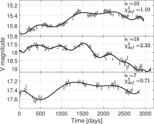
Examples of optical light curves and the chosen polynomical fits with |$\chi ^2_{\rm dof}\sim 1$| (top panel), |$\chi ^2_{\rm dof}>1$| (middle panel), and |$\chi ^2_{\rm dof}<1$| (bottom panel). The degree of the polynomial n is also shown in each panel.
We emphasize that the polynomial fit provides a reasonable way for interpolating the light curves, but it does not have predictive power outside the observed time interval. Therefore, as mentioned above, UV data points that do not overlap with the optical were excluded from the fit.
2.4 Periodic sample
We extracted UV light curves and optical spectra for the sample of periodic quasars from G15 and C16. As mentioned above, with the exception of PG 1302-102, which was analysed in D'Orazio et al. (2015b), only five of the periodic sources in G15 have UV spectra. Among those, four do not have multiple UV observations from GALEX and one has multiple observations in nUV, whereas the spectrum covers the fUV band. Therefore, directly testing the Doppler model was not possible for any of the periodic sources. However, for the sub-sample of sources that have UV light curves and optical spectra (55 out of 111 sources in G15 and 13 out of 33 sources in C16), we were still able to assess whether the Doppler boost model is feasible.
More specifically, assuming that both the optical and UV variability are dominated by the effects of relativistic Doppler boost, we inferred the implied UV spectral index from equation (4). We were able to estimate the nUV spectral index for 68 sources and for 27 of these sources we were also able to calculate the fUV spectral index (see also Table 1). For this, we followed the steps described above for fitting the optical spectra with a power law (in the V band for CRTS and the R band for PTF) and finding the relative amplitude of UV and optical variability.13 Subsequently, we compared our estimates including the 1σ uncertainties to the distribution of measured slopes from the control sample to assess whether the inferred spectral slopes correspond to realistic values seen in quasars with similar properties.
As we mentioned above, the Doppler signature is not limited only to the multiwavelength prediction from equation (4). If the emission of the periodic candidates is indeed due to relativistic Doppler boost, the model should explain the entire sinusoidal variability of the optical light curve as well. For the candidates that have at least one optical spectrum (17 from the PTF sample and 94 from the CRTS sample), we additionally checked whether the Doppler model is feasible based only on the optical variability. To perform this check, we computed the ratio of the maximum possible Doppler boost amplitude (for the given parameters of the putative binaries) to the observed optical variability amplitude.
3 RESULTS
3.1 Null hypothesis test in control sample
We tested the null hypothesis that an apparent Doppler boost signature described by equation (4) arises by chance, given the chromatic variability of quasars. For this test, we checked whether the relative variability amplitudes measured directly from the light curves (left-hand side of the equation) are equal (within their 1σ uncertainty) to the relative amplitudes predicted from the Doppler effect, which depends on the respective spectral slopes (right-hand side of the equation). In Fig. 2, we show the measured ratio of the nUV to the optical varibility amplitude, versus the Doppler-boost prediction calculated from the measured spectral slopes, for the 30 quasars for which all necessary data were available. We also show the equality line for comparison, and we indicate the sources for which the variability is consistent with equation (4) by filled symbols. In total, in the nUV band, we found that the variability is consistent with the Doppler prediction in 6 out of 30 quasars. This means that the Doppler boost signature can be observed by chance in |$P(nUV)\equiv 20_{-6}^{+8}$| per cent14 of the quasars in the sample.
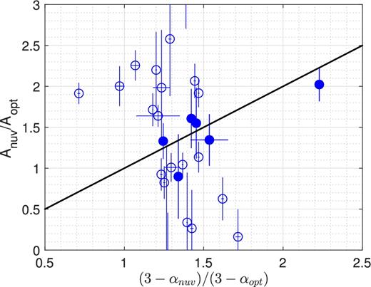
The ratio of variability amplitudes in the nUV and optical bands, measured directly from the light curves versus the amplitudes expected from relativistic Doppler boost, calculated from the measured spectral indices in the two bands. The equality line corresponds to the Doppler-boost prediction from equation (4). The filled symbols indicate sources that are consistent with this Doppler signature within their 1σ error.
We next repeated the above test for quasars in the fUV band. In Fig. 3, we show the amplitude ratio of fUV and optical variability versus the value expected from a Doppler boost in this band. Triangles correspond to data from the COS catalogue, circles to the data from FOS, and the diamond symbol marks the one AGN which was included in both catalogues (the UV slope for this source was calculated as the average slope from the two spectra). Again, we indicate the sources for which variability is consistent with equation (4) by filled symbols. In this case, we found that 6 out of 16 are consistent with equation (4), i.e. an apparent Doppler signature can arise by random chance |$P(fUV)\equiv 37.5_{-11.5}^{+12.5}$| per cent of the time.
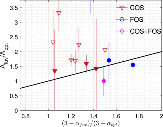
Null hypothesis test for the Doppler boost signature, as in Fig. 2, but in the fUV band. Red triangles correspond to data from the COS catalogue, blue circles to data from FOS and the purple diamond to the one AGN with spectra from both FOS and COS. As in Fig. 2, filled symbols illustrate the sources which satisfy equation (4).
We also note that the data are randomly scattered and do not show any significant correlation. More importantly for our purposes, the overall trends in the data, using either the fUV or the nUV bands, do not follow equation (4), delineated with the equality line. In fact, the Pearson correlation coefficient for the nUV (fUV) sample is −0.23 (−0.69). This is clearly illustrated in Figs 2 and 3, and suggests that the cases which satisfy the Doppler prediction from equation (4) should be due to chance coincidence owing to the limited and noisy data. In other words, the relatively high probability of the Doppler-like signature arising by chance simply reflects limitations of the best available control sample, and not necessarily the intrinsic properties of chromatic AGN variability. The clear conclusion is that higher quality temporally coincident optical and UV light curves and spectra, for a larger number of aperiodic AGN, must be collected in the future.
3.2 Doppler boost in a periodic sample
For a sub-sample of 68 periodic sources (55 from G15 and 13 from C16), which had available UV light curves and optical spectra, we calculated the UV spectral indices that would be required in order for their variability to be consistent with relativistic Doppler boost. For all the above sources, we calculated the spectral index in the nUV band, while for 27 of those (20 from G15 and 7 from C16), we were also able to calculate the spectral slope in the fUV band. Subsequently, we compared the estimated UV indices, including their 1σ error, with the observed distribution of spectral slopes in the respective band in the control sample.
In Figs 4 and 5, we show the inferred nUV and fUV slopes, respectively. We illustrate with circles the sources for which we could calculate the spectral index only in the nUV band, whereas with triangles we show the sources for which both spectral slopes could be calculated. Filled symbols present sources with spectral indices that are consistent within 1σ with the distribution of spectral slopes observed in the control sample (filled circles: only the nUV index was calculated and is consistent; filled triangles: both indices were calculated and both were consistent with the observed distributions) and open symbols present sources with indices that are inconsistent with the observed distributions. In the case that both slopes were determined, open triangles demonstrate sources that are inconsistent in both bands, whereas open diamonds illustrate the sources that are consistent in one band but not in the other. We colour-code the periodic sources from CRTS with blue symbols and the sources from PTF with red. For clarity, we rank-ordered the sources based on their inferred nUV and fUV slope, respectively. The numbers on the right-hand side of the figure refer to the entries in Table 2 below, in which we present the details of the analysis for the periodic sample. On the top panel in both Figs 4 and 5, we show for comparison the distribution of measured UV slopes from the control sample in the respective band. The shaded regions in the bottom panels delineate the full ranges of these distributions.

Top panel: Distribution of nUV spectral indices measured from HST spectra for the sources in the control sample. Bottom panel: Inferred nUV spectral slopes for periodic quasars, assuming Doppler boost variability; filled (open) symbols for spectral indices consistent (inconsistent) with the observed distribution, circles when only the nUV spectral index was calculated, triangles when both nUV and fUV spectral slopes are calculated. We illustrate with open diamonds the sources the spectral indices of which are consistent with the observed slopes in one band but not in the other. Blue symbols present CRTS sources from G15 and red for PTF sources from C16. The indices on the right-hand side of the plot refer to the entries in Table 2. The shaded region delineates the range of the observed distribution shown in the top panel.
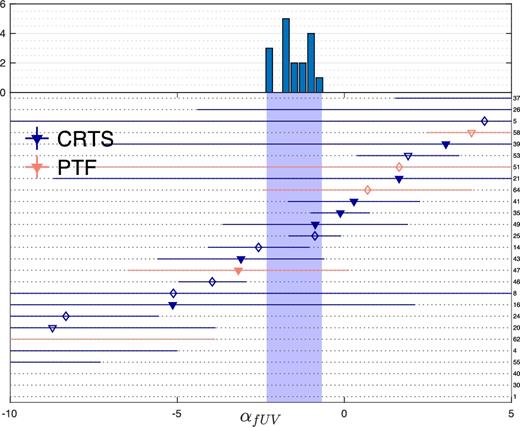
Same as Fig. 4, but in the fUV, instead of the nUV. All the sources in this sample have inferred spectral slopes in both UV bands.
Properties of periodic quasars analysed for relativistic Doppler boost.
| # | Name | Aopt | αopt | AnUV/Aopt | αnUV | AfUV/Aopt | αfUV | |$\frac{A_{\rm Dop}|_{\text{max}}}{2 A_{\rm opt}}$| |
|---|---|---|---|---|---|---|---|---|
| 1 | SDSS J110554.78+322953.7 | 0.11 ± 0.009 | −1.56 ± 0.09 | 5.91 ± 0.71 | −23.94 ± 3.24 | 7.80 ± 1.82 | −32.56 ± 8.29 | 1.62 |
| 2 | SDSS J131706.19+271416.7 | 0.12 ± 0.011 | −0.27 ± 0.12 | 7.61 ± 4.96 | −21.92 ± 16.25 | – | – | 5.45 |
| 3 | SDSS J072908.71+400836.6 | 0.06 ± 0.005 | −3.67 ± 0.01 | 3.70 ± 2.48 | −21.72 ± 16.52 | – | – | 0.65 |
| 4 | 3C 298.0 | 0.08 ± 0.005 | −1.15 ± 0.01 | 5.18 ± 0.72 | −18.49 ± 2.98 | 3.97 ± 2.04 | −13.47 ± 8.48 | 6.44 |
| 5 | SDSS J114438.34+262609.4 | 0.16 ± 0.013 | −1.16 ± 0.01 | 4.12 ± 1.05 | −14.14 ± 4.38 | −0.29 ± 5.10 | 4.19 ± 21.20 | 3.18 |
| 6 | SDSS J081133.43+065558.1 | 0.18 ± 0.014 | −1.37 ± 0.01 | 3.26 ± 0.28 | −11.26 ± 1.22 | – | – | 2.81 |
| 7 | SDSS J153636.22+044127.0 | 0.09 ± 0.008 | −1.01 ± 0.01 | 3.31 ± 0.75 | −10.30 ± 3.02 | – | – | 3.20 |
| 8 | BZQ J0842+4525 | 0.10 ± 0.005 | −1.46 ± 0.01 | 2.46 ± 0.89 | −7.98 ± 3.96 | 1.82 ± 2.30 | −5.12 ± 10.27 | 5.34 |
| 9 | SDSS J140704.43+273556.6 | 0.11 ± 0.007 | −0.58 ± 0.01 | 2.92 ± 0.70 | −7.46 ± 2.51 | – | – | 6.59 |
| 10 | SDSS J130040.62+172758.4 | 0.30 ± 0.022 | −0.65 ± 0.01 | 2.63 ± 0.68 | −6.61 ± 2.50 | – | – | 0.86 |
| 11 | SDSS J131909.08+090814.7 | 0.13 ± 0.011 | −0.90 ± 0.01 | 2.41 ± 1.09 | −6.41 ± 4.23 | – | – | 2.10 |
| 12 | SDSS J125414.23+131348.1 | 0.16 ± 0.012 | −0.08 ± 0.06 | 3.04 ± 0.40 | −6.37 ± 1.24 | – | – | 1.42 |
| 13 | SDSS J142301.96+101500.1 | 0.14 ± 0.010 | −1.29 ± 0.05 | 2.18 ± 0.73 | −6.35 ± 3.15 | – | – | 4.08 |
| 14 | QNZ 3:54 | 0.19 ± 0.013 | −0.74 ± 0.18 | 2.48 ± 0.15 | −6.26 ± 0.57 | 1.49 ± 0.41 | −2.57 ± 1.52 | 2.25 |
| 15 | SDSS J104941.01+085548.4 | 0.16 ± 0.009 | −0.64 ± 0.01 | 2.42 ± 0.39 | −5.81 ± 1.43 | – | – | 2.86 |
| 16 | SDSS J082121.88+250817.5 | 0.09 ± 0.007 | 0.17 ± 0.01 | 2.98 ± 1.26 | −5.45 ± 3.56 | 2.87 ± 2.56 | −5.14 ± 7.24 | 4.21 |
| 17 | SDSS J081617.73+293639.6 | 0.14 ± 0.012 | −0.85 ± 0.01 | 2.15 ± 0.54 | −5.29 ± 2.10 | – | – | 4.51 |
| 18 | SDSS J133654.44+171040.3 | 0.13 ± 0.010 | −1.14 ± 0.01 | 1.94 ± 0.41 | −5.04 ± 1.71 | – | – | 3.50 |
| 19 | SDSS J102255.21+172155.7 | 0.13 ± 0.014 | −0.99 ± 0.12 | 1.96 ± 0.37 | −4.81 ± 1.49 | – | – | 1.79 |
| 20 | SDSS J083349.55+232809.0 | 0.09 ± 0.008 | −1.21 ± 0.01 | 1.71 ± 0.47 | −4.21 ± 1.96 | 2.79 ± 1.16 | −8.74 ± 4.88 | 6.11 |
| 21 | SDSS J104430.25+051857.2 | 0.09 ± 0.007 | −1.05 ± 0.01 | 1.72 ± 0.94 | −3.96 ± 3.81 | 0.34 ± 2.56 | 1.64 ± 10.35 | 5.06 |
| 22a | SDSS J170942.58+342316.2 | 0.18 ± 0.014 | −1.56 ± 0.01 | 1.48 ± 1.13 | −3.77 ± 5.17 | – | – | 4.93 |
| 23 | HS 0926+3608 | 0.08 ± 0.006 | −0.39 ± 0.08 | 1.98 ± 1.20 | −3.73 ± 4.07 | – | – | 9.11 |
| 24 | RXS J10304+5516 | 0.08 ± 0.008 | −0.48 ± 0.01 | 1.92 ± 0.66 | −3.67 ± 2.28 | 3.26 ± 0.80 | −8.34 ± 2.78 | 2.33 |
| 25 | SDSS J121018.34+015405.9 | 0.12 ± 0.009 | −0.22 ± 0.01 | 1.91 ± 0.24 | −3.14 ± 0.76 | 1.21 ± 0.24 | −0.88 ± 0.79 | 1.45 |
| 26 | SDSS J092911.35+203708.5 | 0.21 ± 0.014 | −0.22 ± 0.01 | 1.87 ± 1.81 | −3.03 ± 5.84 | −0.65 ± 2.95 | 5.11 ± 9.51 | 2.76 |
| 27 | SDSS J224829.47+144418.0 | 0.32 ± 0.019 | 0.39 ± 0.01 | 2.25 ± 0.26 | −2.88 ± 0.68 | – | – | 0.61 |
| 28 | SDSS J104758.34+284555.8b | 0.30 ± 0.018 | −0.32 ± 0.01 | 1.73 ± 0.73 | −2.76 ± 2.43 | – | – | 0.65 |
| 29 | SDSS J144754.62+132610.0b | 0.17 ± 0.015 | 0.25 ± 0.01 | 1.99 ± 0.32 | −2.47 ± 0.87 | – | – | 0.85 |
| 30 | SDSS J161013.67+311756.4 | 0.09 ± 0.006 | −0.99 ± 0.01 | 1.36 ± 0.96 | −2.45 ± 3.82 | 6.99 ± 2.74 | −24.93 ± 10.94 | 1.38 |
| 31 | SDSS J094450.76+151236.9 | 0.11 ± 0.008 | −0.18 ± 0.08 | 1.62 ± 0.57 | −2.16 ± 1.83 | – | – | 4.24 |
| 32 | SDSS J121457.39+132024.3 | 0.20 ± 0.012 | −0.50 ± 0.01 | 1.47 ± 0.15 | −2.14 ± 0.53 | – | – | 2.09 |
| 33 | SDSS J082926.01+180020.7b | 0.22 ± 0.015 | −0.20 ± 0.01 | 1.57 ± 0.57 | −2.02 ± 1.89 | – | – | 0.84 |
| 34 | SDSS J154409.61+024040.0 | 0.27 ± 0.018 | −1.25 ± 0.01 | 1.12 ± 0.25 | −1.77 ± 1.06 | – | – | 1.13 |
| 35 | SDSS J140600.26+013252.2b | 0.16 ± 0.014 | 0.07 ± 0.01 | 1.56 ± 0.19 | −1.58 ± 0.54 | 1.07 ± 0.30 | −0.12 ± 0.89 | 0.81 |
| 36 | SDSS J170616.24+370927.0 | 0.13 ± 0.012 | −1.15 ± 0.01 | 1.08 ± 0.22 | −1.47 ± 0.91 | – | – | 2.99 |
| 37 | SDSS J121018.66+185726.0 | 0.08 ± 0.008 | −0.95 ± 0.01 | 0.97 ± 1.15 | −0.82 ± 4.56 | −2.47 ± 2.85 | 12.77 ± 11.25 | 6.52 |
| 38 | HS 1630+2355 | 0.08 ± 0.004 | −0.78 ± 0.01 | 0.95 ± 0.44 | −0.60 ± 1.68 | – | – | 6.34 |
| 39 | SDSS J160730.33+144904.3 | 0.12 ± 0.010 | 0.06 ± 0.01 | 1.20 ± 1.02 | −0.52 ± 3.00 | −0.01 ± 3.48 | 3.04 ± 10.21 | 4.24 |
| 40 | SDSS J221016.97+122213.9 | 0.22 ± 0.017 | 0.33 ± 0.01 | 1.25 ± 0.25 | −0.34 ± 0.68 | 7.85 ± 1.93 | −17.95 ± 5.15 | 1.05 |
| 41 | SDSS J150450.16+012215.5 | 0.14 ± 0.009 | −1.78 ± 0.01 | 0.67 ± 0.19 | −0.22 ± 0.93 | 0.57 ± 0.41 | 0.28 ± 1.98 | 3.58 |
| 42a | SDSS J171617.49+341553.3 | 0.14 ± 0.012 | −0.38 ± 0.02 | 0.95 ± 0.99 | −0.20 ± 3.34 | – | – | 6.07 |
| 43 | US 3204 | 0.20 ± 0.013 | −0.80 ± 0.01 | 0.84 ± 0.29 | −0.18 ± 1.11 | 1.60 ± 0.66 | −3.10 ± 2.50 | 1.61 |
| 44 | SDSS J133631.45+175613.8 | 0.14 ± 0.011 | −0.14 ± 0.02 | 0.94 ± 1.69 | 0.06 ± 5.29 | – | – | 1.66 |
| 45 | SDSS J135225.80+132853.2 | 0.11 ± 0.007 | −0.13 ± 0.02 | 0.93 ± 1.20 | 0.09 ± 3.77 | – | – | 1.61 |
| 46 | UM 234 | 0.17 ± 0.011 | −0.34 ± 0.01 | 0.83 ± 0.19 | 0.23 ± 0.63 | 2.08 ± 0.30 | −3.96 ± 1.01 | 1.70 |
| 47a | SDSS J231733.66+001128.3 | 0.23 ± 0.006 | −0.38 ± 0.01 | 0.79 ± 0.15 | 0.32 ± 0.54 | 1.82 ± 0.97 | −3.17 ± 3.32 | 1.64 |
| 48 | SDSS J124157.90+130104.1 | 0.21 ± 0.015 | −1.38 ± 0.02 | 0.61 ± 0.28 | 0.35 ± 1.23 | – | – | 1.77 |
| 49 | SDSS J082716.85+490534.0b | 0.24 ± 0.019 | 0.05 ± 0.01 | 0.69 ± 0.21 | 0.96 ± 0.62 | 1.31 ± 0.94 | −0.87 ± 2.77 | 0.94 |
| 50a | SDSS J005158.83-002054.1 | 0.21 ± 0.009 | 0.08 ± 0.01 | 0.65 ± 0.43 | 1.09 ± 1.26 | – | – | 1.53 |
| 51a | SDSS J212939.60+004845.5 | 0.21 ± 0.014 | 0.04 ± 0.01 | 0.63 ± 0.16 | 1.13 ± 0.46 | 0.46 ± 3.26 | 1.64 ± 9.67 | 2.93 |
| 52 | SDSS J103111.52+491926.5 | 0.08 ± 0.008 | −1.21 ± 0.01 | 0.36 ± 0.59 | 1.51 ± 2.48 | – | – | 4.83 |
| 53 | SDSS J143820.60+055447.9 | 0.23 ± 0.016 | −0.01 ± 0.01 | 0.35 ± 0.30 | 1.95 ± 0.91 | 0.36 ± 0.51 | 1.91 ± 1.53 | 0.50 |
| 54a | PDS 898 | 0.27 ± 0.011 | 0.42 ± 0.01 | 0.38 ± 0.12 | 2.01 ± 0.30 | – | – | 1.01 |
| 55 | PGC 3096192 | 0.08 ± 0.009 | −0.39 ± 0.01 | 0.09 ± 0.39 | 2.70 ± 1.32 | 5.86 ± 2.83 | −16.88 ± 9.58 | 0.75 |
| 56 | SDSS J084146.19+503601.1 | 0.19 ± 0.013 | 0.61 ± 0.01 | 0.09 ± 0.24 | 2.79 ± 0.58 | – | – | 0.28 |
| 57 | SDSS J164452.71+430752.2 | 0.13 ± 0.011 | −1.20 ± 0.07 | −0.02 ± 0.70 | 3.07 ± 2.92 | – | – | 7.34 |
| 58a | UM 269 | 0.34 ± 0.006 | −0.52 ± 0.01 | −0.02 ± 0.29 | 3.09 ± 1.02 | −0.23 ± 0.39 | 3.80 ± 1.36 | 0.69 |
| 59 | SDSS J152157.02+181018.6 | 0.12 ± 0.011 | −0.64 ± 0.01 | −0.33 ± 0.66 | 4.21 ± 2.40 | – | – | 0.98 |
| 60 | HS 0946+4845 | 0.12 ± 0.007 | 0.01 ± 0.01 | −0.54 ± 0.32 | 4.63 ± 0.95 | – | – | 1.39 |
| 61a | SDSS J235958.72+003345.3 | 0.22 ± 0.012 | −1.43 ± 0.01 | −0.38 ± 0.29 | 4.66 ± 1.28 | – | – | 2.87 |
| 62a | SDSS J024442.77-004223.2 | 0.29 ± 0.018 | −0.81 ± 0.04 | −0.45 ± 0.14 | 4.72 ± 0.52 | 4.31 ± 2.51 | −13.42 ± 9.55 | 0.87 |
| 63a | SDSS J141004.41+334945.5 | 0.21 ± 0.006 | 0.26 ± 0.01 | −0.71 ± 0.24 | 4.94 ± 0.67 | – | – | 1.40 |
| 64a | SDSS J235928.99+170426.9 | 0.35 ± 0.019 | 0.51 ± 0.01 | −1.07 ± 0.40 | 5.66 ± 0.99 | 0.93 ± 1.26 | 0.69 ± 3.13 | 0.99 |
| 65 | SDSS J133516.17+183341.4 | 0.12 ± 0.011 | −0.86 ± 0.01 | −0.84 ± 0.93 | 6.22 ± 3.58 | – | – | 4.83 |
| 66a | SDSS J214036.77+005210.1 | 0.17 ± 0.012 | −0.34 ± 0.24 | −0.97 ± 0.64 | 6.25 ± 2.13 | – | – | 2.62 |
| 67 | SDSS J123147.27+101705.3 | 0.24 ± 0.016 | −0.31 ± 0.01 | −2.18 ± 1.21 | 10.23 ± 4.00 | – | – | 1.38 |
| 68a | SDSS J171122.67+342658.9 | 0.33 ± 0.020 | 0.06 ± 0.01 | −3.08 ± 1.15 | 12.03 ± 3.38 | – | – | 1.44 |
We emphasize with bold the sources that are consistent with relativistic Doppler boost.
Notes:aSMBHB candidates identified in PTF (C16).
bSources that were consistent with the multiwavelength prediction of Doppler boost, but not with the maximum amplitude requirement.
We found that 31 out of 68 sources (or |$46_{-6}^{+6}\,\,\rm{per\,\,cent}$|) are consistent with the observed distribution if we consider only the nUV slopes, and 15 out of 27 (or |$55_{-9}^{+10}\,\,\rm{per\,\,cent}$|) when considering only the fUV spectral indices. If we require that both measured spectral indices are consistent with their respective observed distributions, then we find 9 out of 27 sources (or |$33_{-8}^{+10}\,\,\rm{per\,\,cent}$|) pass both tests. These fractions are higher than expected based on the random multiwavelength variability found above. This test, of course, can be used only to rule out the Doppler hypothesis for approximately two-thirds of the sample. Although the remaining approximately one-third of the sample remains consistent with the Doppler boost, it is necessary to obtain their UV spectra, and directly measure their spectral slopes, to check this. Another caveat is that we are comparing to the distribution observed in our small control sample; the entire population of quasars likely has a wider distribution of spectral slopes. Therefore, it is possible that we excluded some sources that could be Doppler boosted. In principle, this slope-distribution could be measured for many more sources beyond the control sample we assembled, i.e. objects with available UV spectra but without a suitable UV light curve.
Finally, we calculated whether the observed optical variability amplitude is consistent with the maximum value allowed by a relativistic Doppler boost (equation 12). We found that for 76 out of 94 sources from G15 and 18 out of 25 from C16 the ratio is above unity and thus the Doppler boost model is feasible. We show the estimated ratio in Table 2. We were able to exclude five additional sources, which, based on the spectral indices, could be consistent with the Doppler model (filled symbols in the figures above), because they failed this criterion (i.e. the ratio is below unity). This clearly demonstrates that tests of the Doppler model should not be limited to the relative amplitudes from equation (4), but should require the model to explain the overall optical and UV variability of the sources to begin with.
4 DISCUSSION
4.1 Expanding the sample size: UV spectral slope from photometric data?
One of the main limitations of this study is the small size of the sample for which the test was feasible: all of the necessary spectral and photometric information was available only for 42 sources. As mentioned above, this is primarily driven by the lack of UV spectra. On the other hand, for many of the sources without a UV spectrum, photometric data exists in the two UV bands of GALEX. It is therefore natural to ask if we could obtain reliable estimates of the UV spectral slopes for these sources (e.g. by using spectral templates), and thereby increase the sample size significantly.
Under the approximation that the continuum throughout the entire UV band can be described by a single power law, a single GALEX observation with simultaneous photometric measurements in both the nUV and fUV bands determines the power-law slope. Such measurements are available for a large number of quasars and AGN. We assessed the validity of this approach, using the sources in the control sample, by calculating spectral indices from the photometry and comparing with the measured slopes.
In Fig. 6, we present these photometric estimates of the spectral indices versus the true slopes measured directly from HST spectra. Dark blue circles and light blue diamonds indicate data from the FOS catalogue in the nUV and fUV bands, respectively, and red triangles show fUV data from the COS catalogue. The equality line is also shown for comparison. We see that the slopes inferred from photometry are not strongly correlated with the slopes measured directly from the spectra. The spectral slopes tend to be overestimated compared to the measured ones in the nUV band and underestimated in the fUV band. Since the slope calculated from photometry is roughly similar to the average of the spectral slopes in the two bands, this trend is not surprising given that the spectra tend to be steeper in the nUV band and relatively flatter in the fUV band.15
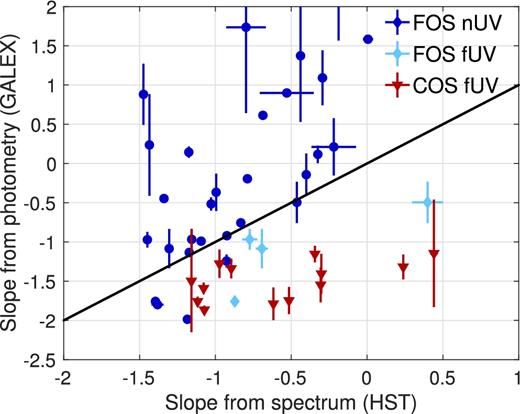
Spectral slopes estimated from GALEX photometric data versus measured by fitting HST spectra with a power law. Dark blue circles: nUV spectra from FOS; light-blue diamonds: fUV spectra from FOS; red triangles: fUV spectra from COS.
While in principle, a more complicated spectral template (in place of a single power law) could account for this curvature, the large scatter in Fig. 6 clearly precludes accurate photometric estimates. The large scatter may be partly caused by the presence of broad emission lines, which affect the calculation of the photometric fluxes and thus the spectral indices. Depending on the redshift of the source, a different set of lines is present in each of the broad-band filters of GALEX and since our sample covers a wide redshift range, it is complicated to account for this effect.
Another possibility would be to calculate the UV spectral indices from spectral templates (e.g. Shull, Stevans & Danforth 2012; Ivashchenko, Sergijenko & Torbaniuk 2014). However, as shown in Figs 4 and 5, the observed distribution of measured spectral slopes is relatively broad. Additionally, the variance of the spectral indices observed in quasars with multiple spectra (mainly optical) is significant. Hence, we expect that using a spectral template will not be sufficient for this study, since it will not allow us to capture the spectral variability of each quasar, which is crucial for our test.
For all the above reasons, we concluded that the expansion of the sample using spectral slopes estimated from photometry is not possible. However, we expect that the test will be feasible for a larger sample of quasars in the near future, once the co-added spectra from STIS and the nUV spectra from COS become available in HSLA. A complementary approach is to acquire UV spectroscopy for a sample of quasars that already have well-sampled UV and optical light curves. In fact, this may be the most time-efficient strategy to improve the null hypothesis test presented here: acquiring well-sampled UV/optical light curves for quasars that have UV and optical spectra would require multiyear campaigns, whereas UV spectra (and potentially optical spectra as well) for the already well-sampled light curves could be obtained without a long wait.
4.2 Null test in both UV bands
In Section 3.1, we showed that the probability for the Doppler signature from equation (4) to occur by random chance is |$P({\rm nUV})=20_{-6}^{+8}$| per cent and |$P({\rm fUV})=37.5_{-11.5}^{+12.5}$| per cent for the samples examined in the nUV and fUV bands, respectively. However, there are four sources in the control sample, for which the null hypothesis test was feasible in both bands. Of these, one is consistent with equation (4) in both bands, one is not consistent in either band and the remaining two are consistent with the Doppler signature only in the fUV band, but not in the nUV band. From this sample, we can conclude that the probability that the Doppler signature from equation (4) can arise by chance in both bands simultaneously is |$P({\rm nUV}\cap {\rm fUV})=25_{-15}^{+25}$| per cent. It is also worth noting that the source which is consistent with the Doppler signature in both bands is the only source which has two fUV spectra from FOS and COS and the spectral index is calculated as the average of the two. If we consider only the FOS spectrum (in the other three cases, both the nUV and fUV slopes are calculated from the same co-added spectra from FOS), the source is inconsistent with equation (4) in the fUV.
As this last point illustrates, in this sub-sample, we are particularly limited by a small number of statistics and sparse data; this unfortunately precludes drawing conclusions from four sources about the entire quasar population. We note further that stochastic variations in the nUV and fUV spectral slopes are likely to be correlated, and this correlation would need to be quantified and taken into account, when performing a joint null-test in the nUV and fUV bands. This joint test would be valuable, since the Doppler model, in principle, should account for variability in both UV bands. It would therefore be particularly important to obtain simultaneous nUV and fUV data on a larger set of objects.
4.3 Variability amplitudes
As mentioned above, another major limitation in this study arises from the very sparse UV light curves. Most of the GALEX light curves have only 2–3 distinct epochs temporally coincident with the optical baseline. This strongly affects the estimates of the relative amplitudes, as is demonstrated by the large error bars in Figs 2 and 3. This limitation is more severe in the fUV band, where the light curves rarely sample more than two epochs, and the photometric uncertainties are larger. In fact, the larger uncertainties in the relative amplitudes, in combination with the smaller sample size, likely explains why the Doppler signature can be observed by chance more often in the fUV band (i.e. ∼20 per cent in nUV versus ∼37 per cent in fUV).
Because of the small number of UV observations, our ability to constrain the UV/optical amplitudes can also be limited by ‘unfortunate’ sampling. In order to illustrate this, consider a UV light curve with only two epochs and the following extreme cases: (1) the UV data points correspond to two epochs with very similar optical magnitudes and (2) the UV data points trace the maximum and minimum magnitude of the optical light curve. In the first case, it is almost impossible to constrain the relative UV/optical amplitude, whereas in the latter case, the amplitude is uniquely constrained. This is an additional uncertainty incorporated into the large error bars in Figs 2 and 3.
Finally, for the available light curves, the optical and UV data were not taken simultaneously. This further limits our ability to estimate the relative variability amplitudes, because quasars show short-term variability (e.g. Kelly et al. 2009).16 This is not included in our analysis, because our polynomial fits effectively filter out the short-term variability of the optical light curves. However, constructing light curves with simultaneous measurements in optical and UV bands, which can be attained with an instrument like the Ultraviolet/Optical Telescope (UVOT) on Swift, can mitigate this issue and significantly improve our UV/optical fits. Note that in the Doppler boost model, this short-term variability can be explained only if the rest-frame luminosities of the mini-discs fluctuate, e.g. due to variable accretion rate.
4.4 Constant spectral slope
Throughout our analysis, we assumed that the spectral slopes do not evolve with time. An intrinsically time-variable spectral slope could, in principle, be easily incorporated in the Doppler-boost model. However, in practice, the assumption of a constant intrinsic spectrum is necessary, because of the lack of multiple UV and optical spectra for each source.17 Since the ultimate goal is to assess whether we can differentiate the Doppler-boost variability from the intrinsic chromatic variability, it is crucial to understand the importance of this limitation.
To investigate this issue, we consider the sample of quasars that have multiple spectroscopic observations. There are seven sources with more than one spectrum in the optical, and one source with two fUV spectra. In Figs 2 and 3, these sources can be recognized from their large horizontal error bars (the error in the spectral slope from a single spectrum is typically small, as seen in the figures for the other sources). From these figures, we conclude that the error introduced by a variable spectral slope is significantly smaller compared to the uncertainty in constraining the relative amplitudes.
4.5 Further improvements of the Doppler tests
Since the chromatic variability of quasars does not appear correlated with the Doppler prediction from equation (4), it is reasonable to assume that with good-quality data (a sufficient number of data points, low photometric noise, simultaneous optical and UV spectra) the variability caused by relativistic Doppler boost could be distinguished much more easily from intrinsic variability. In other words, our main result, namely that the Doppler signature can arise by chance as often as in ∼20 per cent (∼37 per cent) of quasars in the nUV (fUV) bands, likely reflects mainly the limited quality of the currently available data.
A significant improvement could be achieved by increasing the size of the control sample, especially if we can increase the number of sources for which the null hypothesis can be tested simultaneously in both the nUV and fUV bands. In this study, we assembled the control sample starting from the sources that already had measured UV spectra. However, as discussed in Section 2.1 the requirement for UV light curves coincident with the optical baseline was yet another major limitation on the size of the control sample. Likewise, a further limitation results from the large error bars in fitting the relative amplitudes of the optical and UV light curves, mainly due to the small number of UV data points. These limitations could be addressed by first assembling a sample of quasars that have well-sampled UV light curves (in both nUV and fUV) temporally coincident with existing optical light curves, and then obtain UV spectra for these sources, covering both bands.
Finally, in order to incorporate additional uncertainties arising from the short-time variability of quasars, we could start from quasars that have good-quality UV spectra, and then construct well-sampled optical and UV light curves with simultaneous observations. This can be achieved with a telescope such as UVOT on the Swift satellite. However, this would generally require a long wait; i.e. a multiyear campaign to build up reasonably long baselines.
5 SUMMARY
Relativistic Doppler boost is inevitable in compact SMBHBs, and provides a unique multi-wavelength test for the binary nature of any SMBHB candidate. Here we examined this test in the context of binary candidates identified as quasars with periodic optical variability. Our main conclusions can be summarized as follows.
We assembled a control sample of 42 quasars with aperiodic variability, and analysed it to test whether the Doppler boost signature is distinct from intrinsic chromatic brightness variability.
We found that in the best available control sample, variability consistent with the Doppler model can arise by chance for ∼20 per cent and ∼37 per cent of the quasars in the nUV and fUV bands, respectively. The larger chance of coincidence is likely explained by the poorer quality of the fUV data.
For 68 SMBHB candidates identified as quasars with periodic variability, based on their optical/UV light curves and optical spectra, we calculated the UV spectral slopes that would be required for the periodicity to be caused by relativistic Doppler boost.
Of these, 26 sources could be explained by relativistic Doppler boost, since their inferred slopes are consistent with the observed range of spectral indices from the control sample.
We were additionally able to exclude five of the above sources, because even the most optimistic Doppler model cannot produce variability amplitudes as large as observed in the optical.
Overall, our paper suggests that quasars do not often mimic the optical/UV colour variations expected to arise from relativistic Doppler boost. We have also demonstrated the need for a larger and better control sample. With a sufficient number of UV data points, low photometric noise, and simultaneous optical and UV spectra, such an improved control sample could be constructed, and would allow an improved test, conclusively ruling out that a Doppler colour signature arises by chance from stochastic intrinsic variability.
ACKNOWLEDGEMENTS
We thank Jules Halpern, Szabi Marka, Imre Bartos, Joe Lazio, Michele Vallisneri, and Matthew Graham for useful discussions and suggestions. MC acknowledges support from the National Science Foundation (NSF) NANOGrav Physics Frontier Center, award number 1430284. Financial support was provided by NASA through grants NNX15AB19G, NNX17AL82G, and 16-SWIFT16-0015, and by NSF grant 1715661. Financial support to DJD was provided from NASA through Einstein Postdoctoral Fellowship award number PF6-170151. ZH also gratefully acknowledges support from a Simons Fellowship in Theoretical Physics and hospitality by NYU.
Footnotes
This quasar was also included in the sample analysed in G15, but was not identified as periodic. The shortest periodic component of ∼740 d was identified with both the wavelet and the autocorrelation function analysis in G15, but did not have enough power to be classified as periodic, potentially due to the second periodic component (M. Graham, private communication).
The periodicity search algorithms and statistical analyses in these papers differ significantly. However, in all cases, the underlying assumption for the quasar variability is the DRW model.
The X-ray luminosity also arises very close to SMBHs and in the binary scenario, it may be Doppler boosted. In this paper, we will focus only on the optical/UV variability, because the available X-ray data are insufficient to extend our study to this band.
For this test, the Doppler signature refers to the multiwavelength variability amplitudes described in equation (4). However, we emphasize that the Doppler model does not refer only to the relative amplitudes, but it can explain the overall variability, e.g. for a circular binary orbit, it can explain the sinusoidal light curve.
We only considered UV light curves consisting of at least two distinct epochs, separated by 100 days within the optical baseline (see below).
Light curves in optical and UV bands, as well as optical spectra, are available for very large samples of quasars from CRTS, GALEX, and SDSS, respectively.
To the best of our knowledge, the above are the only available catalogues with high-level quasar and AGN spectra. Calibrated nUV spectra from COS, and from the Space Telescope Imaging Spectrograph (STIS) will be released in the future in the HSLA (https://hla.stsci.edu).
For these last four sources, the test was feasible in both the fUV and nUV bands.
Since the optical light curves of the periodic sources are described by sinusoids, when fitting the UV light curves, we included UV data points outside of the optical baseline. This was not possible for the stochastic variability of quasars in the control sample.
We calculated the 1σ confidence intervals with the Wilson (score) method (Wilson 1927).
We note that the spectral slopes βλ are typically negative, as is also obvious from the figure.
Short-term variability here refers to time-scales of several days to a couple of months and not the variability between 1 and 10 d which Caplar, Lilly & Trakhtenbrot 2017 found to be overestimated due to the limited photometric precision of the time domain surveys.
In the ideal case, we would test the Doppler signature with simultaneous UV and optical spectra.
REFERENCES
