


Abstract
We present a study of observed Type II supernova (SN II) colours using optical/near-infrared photometric data from the Carnegie Supernovae Project-I. We analyse four colours (B − V, u − g, g − r, and g − Y) and find that SN II colour curves can be described by two linear regimes during the photospheric phase. The first (s1, colour) is steeper and has a median duration of ∼40 d. The second, shallower slope (s2, colour) lasts until the end of the ‘plateau’ (∼80 d). The two slopes correlate in the sense that steeper initial colour curves also imply steeper colour curves at later phases. As suggested by recent studies, SNe II form a continuous population of objects from the colour point of view as well. We investigate correlations between the observed colours and a range of photometric and spectroscopic parameters including the absolute magnitude, the V-band light-curve slopes, and metal-line strengths. We find that less luminous SNe II appear redder, a trend that we argue is not driven by uncorrected host-galaxy reddening. While there is significant dispersion, we find evidence that redder SNe II (mainly at early epochs) display stronger metal-line equivalent widths. Host-galaxy reddening does not appear to be a dominant parameter, neither driving observed trends nor dominating the dispersion in observed colours. Intrinsic SN II colours are most probably dominated by photospheric temperature differences, with progenitor metallicity possibly playing a minor role. Such temperature differences could be related to differences in progenitor radius, together with the presence or absence of circumstellar material close to the progenitor stars.
1 INTRODUCTION
The community of supernova (SN) researchers is now experiencing a growing interest in the study of core-collapse supernovae (CC SNe), after focusing more on the well-studied Type Ia supernovae (hereafter SNe Ia; Minkowski 1941; Elias et al. 1985) for 20 yr. CC SNe are believed to be the explosions of massive stars at the end of their lives (≥8 M⊙; see Smartt et al. 2009 for a review). CC SNe exhibit a large range of observed photometric and spectroscopic properties. They can be first subclassified according to the absence or the presence of H i lines: SNe Ib/c and SNe II, respectively (see e.g. Filippenko 1997, and references therein). Secondly, hydrogen-rich CC SNe can be grouped using spectroscopic properties: SNe II with broad, long-lasting Balmer lines in their spectra; SNe IIb, which evolve spectroscopically from SNe II at early times to SNe Ib several weeks past maximum brightness (Woosley et al. 1987; Filippenko 1988; Filippenko et al. 1993), and SNe IIn with relatively narrow emission lines in their spectra (Chevalier 1981; Fransson 1982; Schlegel 1990; Filippenko 1991; Chugai & Danziger 1994).
SNe II,1 the most frequently occurring CC SNe in the Universe (Li et al. 2011; Graur et al. 2017), are the explosions of stars that have retained a significant fraction of their hydrogen envelopes prior to exploding. Thanks to direct progenitor detections and earlier hydrodynamical modelling, most SN II progenitors have been robustly established as the explosions of red supergiants (RSGs; M ≤ 25 M⊙; Grassberg et al. 1971; Falk & Arnett 1977; Chevalier 1976; Van Dyk et al. 2003; Smartt et al. 2009).
SNe II are very useful tools for understanding the composition and evolution of our Universe because they have been established as metallicity (Dessart et al. 2014; Anderson et al. 2016) and distance indicators (e.g. Hamuy & Pinto 2002). Several methods exist to standardize SN II peak brightness and make them useful for cosmology: the ‘expanding photosphere method’ (Kirshner & Kwan 1974; Schmidt et al. 1994; Hamuy et al. 2001; Leonard et al. 2003; Dessart & Hillier 2005, 2006; Jones et al. 2009; Emilio Enriquez et al. 2011; Gall et al. 2016), the ‘standard candle method’ (Hamuy & Pinto 2002; Nugent et al. 2006; D'Andrea et al. 2010; Poznanski et al. 2010; de Jaeger et al. 2017a; Gall et al. 2018), the ‘photospheric magnitude method’ (Rodríguez et al. 2014), and the ‘photometric colour method’ (de Jaeger et al. 2015, 2017b).
Generally, SN II standardization is achieved by adding an observed colour correction to account for reddening of light caused by host-galaxy dust extinction or any intrinsic variation in the magnitude–colour relations. However, with this factor, it is assumed that all SNe II follow the same magnitude–colour law, which has never been proved to be the case. Additionally, by assuming that the colour diversity comes exclusively from dust extinction (which may not be true), such a colour term correction has led the SN Ia and SN II communities to derive surprisingly low total-to-selective extinction ratios (RV) as compared with the Milky Way Galaxy (1.5–2.5; Krisciunas et al. 2007; Elias-Rosa et al. 2008; Goobar 2008; Poznanski et al. 2009; Folatelli et al. 2010; Olivares et al. 2010; Mandel et al. 2011; Phillips et al. 2013; Burns et al. 2014; Rodríguez et al. 2014; de Jaeger et al. 2015). These low RV values could reflect differences in the dust properties, or intrinsic magnitude–colour relations for SNe Ia/SNe II not taken into account in the colour corrections.
Within this context, a more complete understanding of SN II colours would be an asset for cosmological studies while also furthering our knowledge of SN II progenitors and explosion properties. Additionally, as the K-correction (Oke & Sandage 1968; Hamuy et al. 1993; Kim et al. 1996; Nugent et al. 2002) – applied to take into account the expansion of the Universe – strongly depends on colour, understanding SN II colour diversity would help improve its accuracy. To date, there are very few statistical studies of SN II observed colours and how these relate to intrinsic colours or the effects of reddening from the host galaxy.
While the overall SN II colour behaviour (through studies of colour curves) is relatively well known from investigations of individual events such as SN 1999em (Hamuy et al. 2001; Leonard et al. 2002a; Elmhamdi et al. 2003), SN 1999gi (Leonard et al. 2002b), SN 2004et (Sahu et al. 2006; Maguire et al. 2010), SN 2005cs (Pastorello et al. 2009), SN 2007od (Inserra et al. 2011), SN 2013by (Valenti et al. 2015), and SN 2013ej (Valenti et al. 2014; Bose et al. 2015; Huang et al. 2015; Dhungana et al. 2016; Mauerhan et al. 2017), these have yet to be put within the context of the full diversity of SNe II and the progenitor parameters that influence intrinsic colours.
General SN II colour behaviour, as noted by Patat et al. (1994), consists of two regimes with two different slopes and can be described as follows. At early times (∼10 d), a rapid increase of the (B − V) colour is seen as the envelope expands and cools from an initial temperature of >10 000 K to the recombination temperature of hydrogen (∼5500 K). After ∼35 d from the explosion (i.e. during the recombination phase), the colour varies more slowly, since the photospheric temperature is assumed to be the hydrogen recombination temperature. For the redder bands (e.g. V − I), the colour increases more slowly than (B − V) during the photospheric phase, mainly because the spectral energy distribution is less sensitive to temperature changes in the red than in the blue part of the spectrum (see Galbany et al. 2016).
Understanding the origin of the observed diversity in SN II colours is also important for deriving the host-galaxy extinction. One of the commonly used methods to estimate the reddening is to assume that all SN II (B − V) colour curves evolve similarly, and the objects that appear to be offset by a constant are reddened by host-galaxy extinction (Schmidt et al. 1992). Despite the fact that the colours evolve differently, if one assumes that all SN II colours at a given epoch are intrinsically similar (which we argue is not actually the case), the offset is directly related to the amount of dust. To increase the colour uniformity, one should pick an epoch where the physical conditions (mainly the temperature) are similar. However, even if a such an epoch is chosen (e.g. the plateau phase; Faran et al. 2014a), intrinsic differences still exist. For example, Faran et al. (2014b) used an average colour of (a maximum of) 11 slow-declining SNe II (historically SNe IIP) and (a maximum of) 8 fast-declining SNe II (historically SNe IIL). They showed that the fast-declining SNe II are, on average, redder than the slow-declining events. Pastorello et al. (2004) and Spiro et al. (2014), using a sample of low-luminosity SNe II and comparing the colour with a sample of normal SNe II, found that low-luminosity SNe II have intrinsic colours that are unusually red.
Using theoretical models, Kasen & Woosley (2009) confirmed the results of Pastorello et al. (2004); they found a slight trend for brighter models (fast-declining SNe II) to be bluer than fainter models at 50 d after the explosion. Also from a theoretical point of view, Dessart et al. (2013) have tried to explain the intrinsic colour variations with differences in progenitor properties. They showed that the colour evolution of SNe II is primarily driven by different progenitor radii, while the explosion energies have negligible influence. SNe II with more extended progenitors are subject to weaker cooling through expansion and thus tend to be bluer. This latter conclusion was supported by Lisakov et al. (2017), who studied the low-luminosity SN II family and showed that their model with the highest mixing-length parameter employed during stellar evolution produced SNe II that appear redder. The mixing-length parameter and the radius anticorrelate; therefore, this again showed that SNe II with more compact progenitors display redder colours, as the ejecta cool more quickly owing to the effects of expansion. In addition, Lisakov et al. (2017) suggested that the mass-loss rate suffered by the progenitor does not influence the colour.
An additional intrinsic progenitor parameter that is thought to play an important role in SN II colour diversity is metallicity. Progenitor metallicity can affect the observed colours of SNe II in two ways, as shown and discussed by Dessart et al. (2013). First, the metallicity plays a role in the path taken by stellar evolution to produce the pre-SN progenitor. A lower metallicity progenitor will produce a more compact star prior to explosion. Following the above discussion, this will lead to redder SNe II at early times. Secondly, the abundance of metals in the progenitor star's envelope directly affects the strength of metal lines within the spectrum and hence the SN's colour. At lower metallicity, the flux at blue wavelengths is significantly higher owing to the reduced effects of line blanketing, leading to bluer colours for lower metallicity progenitors throughout the photospheric phase.
Finally, during the last few years, a number of studies have claimed that some (and maybe many) SNe II show signs of interaction with circumstellar material (CSM) during the first few days post-explosion (e.g. Khazov et al. 2016; Morozova et al. 2016; Dessart et al. 2017; Moriya et al. 2017; Morozova et al. 2017; Yaron et al. 2017). Such interaction with previously unaccounted material (neither in stellar evolution models nor in SN II explosion models) would provide an additional source of energy and is likely to keep the photosphere at higher temperatures (and therefore bluer colours) for longer periods of time.
In summary, there appear to be three key progenitor parameters that are expected to play important roles in producing intrinsic diversity in SN II colours and their evolution: (1) progenitor radius, (2) progenitor metallicity, and (3) the presence or absence of CSM close to the progenitor stars. How these parameters relate between different progenitors is not clear. Neither is the degree to which the effects of host-galaxy extinction play an important or secondary role in driving observed SN II colours. Such questions can only be answered through the analysis of large samples of events where one can hope to cover as large an area of Nature's parameter space as possible. This drives the motivation of the current study: using a large sample of well-observed SNe II with both photometric and spectral coverage to understand the underlying causes of differences in observed SN II colours, as well as to better understand the SN II colour-term corrections used in cosmological analyses.
For this purpose, we use the Carnegie Supernova Project-I sample (CSP-I; Hamuy et al. 2006; PIs: Phillips & Hamuy), one of the most complete SN II data sets, with optical and near-infrared (NIR) light curves in a well-understood photometric system. We focus our study on the photospheric phase, from the explosion until the SN falls on to the 56Ni decay slope. This is motivated mainly by the lack of data during the nebular phase and because for SN II cosmology, the Hubble diagram is derived for an epoch ∼50 d after the explosion (i.e. during the recombination phase).
The paper is organized as follows. Section 2 contains a brief description of the data set. In Section 3, we show a detailed study of the (B − V) colour-curve properties and search for possible correlations with the photometric/spectroscopic parameters presented by Gutiérrez et al. (2017b), which are a refined version of the parameters discussed by Anderson et al. (2014) and Gutiérrez et al. (2014). Three other colours [(u − g), (g − r), and (g − Y)] are analysed in Section 4, in the same vein as (B − V). In Section 5, the host-galaxy extinction is examined. Finally, in Section 6 we more fully discuss our main results and try to understand them in terms of differences in progenitor properties. We provide our concluding remarks in Section 7. In the Appendix, the reader can find additional plots showing the correlations discussed in the main text.
2 DATA SAMPLE
2.1 Data reduction
In this work, the sample from de Jaeger et al. (2015, 2017b) is used. For this reason, only a brief description of the CSP-I (Hamuy et al. 2006) and the methods used to reduce the data are given in this section.
The CSP-I was a 5-yr (2004–2009) low-redshift SN survey, providing optical and NIR light curves in a well-defined and well-understood photometric system. It was also designed to spectroscopically monitor the majority of the objects. Using the Las Campanas Observatory facilities (the Swope 1 m and the du Pont 2.5 m telescopes), CSP-I succeeded in building a large sample of 69 SNe II, where 49 have both optical and NIR light curves with good temporal coverage (the other 20 SNe II do not have NIR data). From this sample, as described by de Jaeger et al. (2015, 2017b), we excluded four SNe II (SN 2004ej, SN 2005hd, SN 2007X, and SN 2008K) from the analysis. The sample used in this work thus consists of the 65 SNe II listed in Table 1.
SN II (B − V) colour-curve parameters, host-galaxy information, and MW extinction.
| SN | host recession velocity | E(B − V)MW | s1, (B − V) | s2, (B − V) | Ttrans, (B − V) |
|---|---|---|---|---|---|
| (km s−1) | (mag) | (mag 100 d−1) | (mag 100 d−1) | (d) | |
| 2004er | 4411 | 0.0220 | 2.49 (0.10) | 0.32 (0.06) | 48.38 (1.36) |
| 2004fb | 6100 | 0.0546 | ⋅⋅⋅ (⋅⋅⋅) | ⋅⋅⋅ (⋅⋅⋅) | ⋅⋅⋅ (⋅⋅⋅) |
| 2004fc | 1831 | 0.0219 | 2.69 (0.11) | 0.87 (0.08) | 42.11 (2.00) |
| 2004fx | 2673 | 0.0883 | 1.69 (0.24) | 0.50 (0.14) | 36.78 (3.36) |
| 2005J | 4183 | 0.0224 | 2.81 (0.08) | 0.71 (0.04) | 37.66 (0.84) |
| 2005K | 8204 | 0.0340 | 1.63 (0.20) | ⋅⋅⋅ (⋅⋅⋅) | ⋅⋅⋅ (⋅⋅⋅) |
| 2005Z | 5766 | 0.0236 | 3.02 (0.09) | 0.82 (0.11) | 35.13 (1.46) |
| 2005af | 563 | 0.1588 | ⋅⋅⋅ (⋅⋅⋅) | ⋅⋅⋅ (⋅⋅⋅) | ⋅⋅⋅ (⋅⋅⋅) |
| 2005an | 3206 | 0.0819 | 3.41 (0.07) | 1.06 (0.10) | 37.76 (0.68) |
| 2005dk | 4708 | 0.0409 | 3.34 (0.22) | 1.25 (0.05) | 37.31 (0.91) |
| 2005dn | 2829 | 0.0437 | 1.16 (0.16) | 0.40 (0.03) | 34.23 (1.58) |
| 2005dt | 7695 | 0.0248 | 2.28 (0.35) | 0.53 (0.15) | 43.16 (3.91) |
| 2005dw | 5269 | 0.0194 | 2.38 (0.23) | 0.75 (0.12) | 38.25 (2.27) |
| 2005dx | 8012 | 0.0205 | 3.64 (0.20) | 0.98 (0.64) | 30.88 (8.36) |
| 2005dz | 5696 | 0.0691 | 2.22 (0.13) | 0.26 (0.08) | 43.91 (1.70) |
| 2005es | 11287 | 0.0718 | 3.08 (0.44) | ⋅⋅⋅ (⋅⋅⋅) | ⋅⋅⋅ (⋅⋅⋅) |
| 2005gk | 8773 | 0.0482 | 1.25 (0.08) | ⋅⋅⋅ (⋅⋅⋅) | ⋅⋅⋅ (⋅⋅⋅) |
| 2005lw | 7710 | 0.0423 | 4.88 (0.52) | 0.62 (0.45) | 32.55 (2.43) |
| 2005me | 6726 | 0.0203 | 3.18 (0.32) | 0.70 (0.20) | 33.60 (2.36) |
| 2006Y | 10074 | 0.1114 | 1.67 (0.15) | ⋅⋅⋅ (⋅⋅⋅) | ⋅⋅⋅ (⋅⋅⋅) |
| 2006ai | 4571 | 0.1080 | 2.03 (0.06) | ⋅⋅⋅ (⋅⋅⋅) | ⋅⋅⋅ (⋅⋅⋅) |
| 2006bc | 1363 | 0.1762 | 2.34 (0.15) | 0.71 (0.32) | 41.19 (2.70) |
| 2006be | 2145 | 0.0251 | 2.69 (0.05) | 1.01 (0.02) | 31.85 (0.39) |
| 2006bl | 9708 | 0.0435 | 2.63 (0.09) | 1.25 (0.22) | 39.78 (3.64) |
| 2006ee | 4620 | 0.0516 | 2.24 (0.18) | 0.81 (0.14) | 40.57 (2.81) |
| 2006it | 4650 | 0.0850 | 3.30 (0.30) | ⋅⋅⋅ (⋅⋅⋅) | ⋅⋅⋅ (⋅⋅⋅) |
| 2006iw | 9226 | 0.0426 | 3.07 (0.23) | 0.75 (0.20) | 37.87 (2.81) |
| 2006ms | 4543 | 0.0300 | 3.75 (0.44) | ⋅⋅⋅ (⋅⋅⋅) | ⋅⋅⋅ (⋅⋅⋅) |
| 2006qr | 4350 | 0.0384 | 3.06 (0.14) | 0.80 (0.11) | 36.78 (1.54) |
| 2007P | 12224 | 0.0349 | 2.17 (0.15) | ⋅⋅⋅ (⋅⋅⋅) | ⋅⋅⋅ (⋅⋅⋅) |
| 2007U | 7791 | 0.0449 | 3.30 (0.07) | 0.95 (0.24) | 34.75 (2.56) |
| 2007W | 2902 | 0.0443 | 2.73 (0.22) | 0.70 (0.11) | 33.39 (2.30) |
| 2007aa | 1465 | 0.0227 | 1.77 (0.10) | 0.69 (0.06) | 35.89 (1.52) |
| 2007ab | 7056 | 0.2292 | ⋅⋅⋅ (⋅⋅⋅) | ⋅⋅⋅ (⋅⋅⋅) | ⋅⋅⋅ (⋅⋅⋅) |
| 2007av | 1394 | 0.0311 | ⋅⋅⋅ (⋅⋅⋅) | ⋅⋅⋅ (⋅⋅⋅) | ⋅⋅⋅ (⋅⋅⋅) |
| 2007hm | 7540 | 0.0549 | 1.55 (0.20) | 0.47 (0.20) | 32.38 (4.10) |
| 2007il | 6454 | 0.0403 | 2.12 (0.11) | 0.55 (0.09) | 49.14 (2.33) |
| 2007it | 1193 | 0.0994 | 2.64 (0.33) | ⋅⋅⋅ (⋅⋅⋅) | ⋅⋅⋅ (⋅⋅⋅) |
| 2007ld | 8994 | 0.0810 | 2.42 (0.34) | ⋅⋅⋅ (⋅⋅⋅) | ⋅⋅⋅ (⋅⋅⋅) |
| 2007oc | 1450 | 0.0173 | 2.06 (0.11) | 0.72 (0.08) | 37.06 (1.52) |
| 2007od | 1734 | 0.0312 | 2.97 (0.09) | 0.93 (0.03) | 27.07 (0.66) |
| 2007sq | 4579 | 0.1769 | ⋅⋅⋅ (⋅⋅⋅) | 1.41 (0.13) | ⋅⋅⋅ (⋅⋅⋅) |
| 2008F | 5506 | 0.0422 | 1.89 (0.21) | ⋅⋅⋅ (⋅⋅⋅) | ⋅⋅⋅ (⋅⋅⋅) |
| 2008M | 2267 | 0.0389 | 2.30 (0.15) | 0.89 (0.17) | 45.43 (3.52) |
| 2008W | 5757 | 0.0837 | 2.64 (0.39) | 0.98 (0.11) | 32.54 (2.38) |
| 2008ag | 4439 | 0.0713 | 1.38 (0.19) | 0.39 (0.04) | 58.89 (3.49) |
| 2008aw | 3110 | 0.0351 | 2.54 (0.05) | 1.30 (0.06) | 48.14 (1.02) |
| 2008bh | 4345 | 0.0187 | 3.11 (0.24) | 0.98 (0.20) | 37.56 (2.76) |
| 2008bk | 230 | 0.0168 | 2.11 (0.32) | 0.46 (0.04) | 49.38 (1.93) |
| 2008bp | 2723 | 0.0596 | ⋅⋅⋅ (⋅⋅⋅) | ⋅⋅⋅ (⋅⋅⋅) | ⋅⋅⋅ (⋅⋅⋅) |
| 2008br | 3019 | 0.0800 | 3.22 (0.22) | 1.07 (0.05) | 24.56 (1.19) |
| 2008bu | 6630 | 0.3523 | 3.09 (0.45) | ⋅⋅⋅ (⋅⋅⋅) | ⋅⋅⋅ (⋅⋅⋅) |
| 2008ga | 4639 | 0.5639 | ⋅⋅⋅ (⋅⋅⋅) | ⋅⋅⋅ (⋅⋅⋅) | ⋅⋅⋅ (⋅⋅⋅) |
| 2008gi | 7328 | 0.0549 | 2.90 (0.19) | 0.77 (0.31) | 37.84 (2.87) |
| 2008gr | 6831 | 0.0113 | 2.60 (0.12) | 0.73 (0.22) | 38.06 (2.29) |
| 2008hg | 5684 | 0.0158 | 3.31 (0.16) | ⋅⋅⋅ (⋅⋅⋅) | ⋅⋅⋅ (⋅⋅⋅) |
| 2008ho | 3082 | 0.0163 | 2.20 (0.18) | ⋅⋅⋅ (⋅⋅⋅) | ⋅⋅⋅ (⋅⋅⋅) |
| 2008if | 3440 | 0.0281 | 1.96 (0.08) | ⋅⋅⋅ (⋅⋅⋅) | ⋅⋅⋅ (⋅⋅⋅) |
| 2008il | 6276 | 0.0142 | ⋅⋅⋅ (⋅⋅⋅) | ⋅⋅⋅ (⋅⋅⋅) | ⋅⋅⋅ (⋅⋅⋅) |
| 2008in | 1566 | 0.0193 | 2.75 (0.10) | 0.78 (0.15) | 39.86 (2.08) |
| 2009N | 1036 | 0.0182 | 3.06 (0.14) | 0.98 (0.12) | 37.92 (1.84) |
| 2009ao | 3339 | 0.0332 | 1.91 (0.17) | ⋅⋅⋅ (⋅⋅⋅) | ⋅⋅⋅ (⋅⋅⋅) |
| 2009au | 2819 | 0.0785 | 1.91 (0.05) | ⋅⋅⋅ (⋅⋅⋅) | ⋅⋅⋅ (⋅⋅⋅) |
| 2009bu | 3494 | 0.0217 | 2.12 (0.24) | 0.88 (0.12) | 37.44 (3.04) |
| 2009bz | 3231 | 0.0340 | 2.17 (0.08) | 0.95 (0.09) | 36.23 (1.48) |
Notes. Column 1, SN name; Column 2, host-galaxy heliocentric recession velocity taken from the NASA Extragalactic Database (NED: http://ned.ipac.caltech.edu/); Column 3, reddening due to the Milky Way (Schlafly & Finkbeiner 2011), from the NASA/IPAC infrared science archive website (http://irsa.ipac.caltech.edu/cgi-bin/bgTools/nph-bgExec); Columns 4, 5, and 6, the measured colour-curve parameters s1, (B − V), s2, (B − V), and Ttrans, (B − V) (respectively).
All optical images (B, V, u, g, and r) were reduced in a standard manner including bias subtraction, flat-field correction, a linearity correction, and an exposure-time correction for a shutter time delay. The final magnitudes were derived relative to a local sequence of stars and calibrated from observations of standard stars in the Landolt (1992) (BV) and Smith et al. (2002) (ugri) systems.
The NIR images were also reduced following standard steps consisting of dark subtraction, flat-field division, sky subtraction, and geometric alignment and combination of the dithered frames. NIR photometry (Y) was calibrated using standard stars in the Persson et al. (2004) system. For more information about the data processing technique and the different instruments/filters, the reader can refer to Hamuy et al. (2006), Contreras et al. (2010), Stritzinger et al. (2011), and Krisciunas et al. (2017).
All magnitudes are expressed in the natural CSP-I photometric system and are simultaneously corrected for Milky Way (MW) extinction and for the expansion of the Universe (K-correction; Oke & Sandage 1968; Hamuy et al. 1993; Kim et al. 1996; Nugent et al. 2002). All of the steps to make these corrections are fully outlined by de Jaeger et al. (2015, 2017b).
In this work, we use the recalibrated CSP-I photometry that will be published in a definitive CSP-I data paper by Contreras et al. (in preparation). The CSP-I SN II spectroscopy was recently published by Gutiérrez et al. (2017a).
2.2 Host-galaxy extinction
As mentioned in Section 2.1, all magnitudes are corrected for Milky Way Galaxy extinction (AVG) and for the Universe's expansion (K-correction), but not for host-galaxy extinction (AVh). In the literature, there are a handful of methods to estimate reddening. These include the Na i D equivalent width (Munari & Zwitter 1997; Turatto et al. 2003; Poznanski et al. 2011) or the (V − I) colour excess at the end of the plateau (Olivares et al. 2010). However, none of these methods seems to be satisfactory. The accuracy of using the Na i D line in low-resolution spectra (which is indeed the case for the current sample) has been questioned (Poznanski et al. 2011; Phillips et al. 2013; Galbany et al. 2017). For the colour method, we must assume that all SNe II have the same intrinsic colour, which seems not to be true, as we will demonstrate in this work. The validity of these methods has also been questioned by Faran et al. (2014a); using a variety of different host-galaxy extinction estimation methods, they found that when applied to SN II correlations, the dispersion increased. This latter observation was also recently outlined by Gutiérrez et al. (2017b). Therefore, we decided to not correct for AVh because (a) we believe that the extinction is probably not significant for most SNe II in the sample, and (b) any attempts to correct for extinction are likely to simply add additional errors to our colours, given the very uncertain nature of the corrections.
In Section 5, we discuss the effect of the dust extinction in more detail, and in Section 6.6, the ‘intrinsic’ colour dispersion of our sample is further explored. Note that as the K-corrections depend on the colours, we test whether the trends presented in this work are stronger with or without K-corrections. We find that all of the correlations are stronger when the K-corrections are applied, justifying and validating our inclusion of these corrections.
3 (B − V) COLOUR CURVES
In this section, we first analyse the morphology of the (B − V) colour curves, and then compare observed colours at different epochs with a range of V-band photometric and optical spectroscopic parameters as presented by Gutiérrez et al. (2017b). The choice of the (B − V) colour is motivated by the fact that historically, B and V photometry were the most widely obtained, hence allowing easier comparison with previous studies found in the literature. Additionally, in the literature, the host-galaxy extinction is regularly given as the colour excess E(B − V). Finally, note that Anderson et al. (2014) used the V-band light curves in their study.
In this analysis, we use the Pearson test to determine the existence and strength of correlations between our defined colour parameters and other photometric and spectral properties. We perform 10 000 Monte Carlo bootstrapping simulations, and then the mean Pearson value (r) of these 10 000 simulations is calculated and presented in each figure, together with its standard deviation (σ). As in Anderson et al. (2014), we take a conservative approach: in each figure, only the upper limit (i.e. p-value calculated for r-σ) of the probability of finding such a correlation strength by chance is plotted.2 Finally, it is worth noting that in this paper, the colours themselves are linearly interpolated to different epochs.
3.1 Measured parameters
The SN 2005J (B − V) light curve is shown in Fig. 1 together with a schematic of the (B − V) colour-curve parameters chosen for measurement. Looking at the (B − V) colour curves of the whole sample and as noted by Patat et al. (1994), two regimes composed of two different slopes are apparent (see Fig. 1 and Section A1). During the first ∼30–40 d, the object becomes quickly redder as the SN envelope expands and cools. After this first phase, the SN colour changes more slowly as the rate of cooling decreases. Following the notation from Anderson et al. (2014), we defined the following parameters:
s1, (B − V): the first colour rate of change in magnitudes per 100 d since the explosion date (hereafter mag 100 d−1).
s2, (B − V): the second colour rate of change in mag 100 d−1 after Ttrans, (B − V) and until the end of the plateau phase. s2, (B − V) is always observed to be flatter than s1, (B − V) (as first observed by Patat et al. 1994).
Ttrans, (B − V): the epoch in days from explosion of the transition between s1, (B − V) and s2, (B − V).

An example of the (B − V) colour-curve parameters measured for each SN as applied to SN 2005J. The two slopes, s1, (B − V) and s2, (B − V), are, respectively, represented in red and black. The epoch of the transition, Ttrans, (B − V), is indicated with a vertical blue dashed line. These parameters for our full sample are listed in Table 1. The dashed green line represents the power-law fit, (B − V) = 3.894 − 5.694 t−0.177.
To measure the free parameters s1, (B − V), s2, (B − V), and Ttrans, (B − V), we use a python program that consists of performing a weighted least-squares fit of the ‘AK-corrected’ colour curves (MW extinction and K-correction) with one and two slopes. To choose between one or two slopes, an F-test3 is performed. The fit is only done from the explosion date (Gutiérrez et al. 2017b) to the end of the plateau (i.e. during the optically thick phase). When the epoch of the end of the plateau is unknown, we choose 80 d, which is the average value of our sample (Anderson et al. 2014). If the F-test favoured one slope but the first point starts after 35 d past the explosion, we consider the slope as s2, (B − V) and not s1, (B − V), as the transition occurs on average at ∼38 d. Note that we also tried to fit the colour curves using a power law; however, in the majority of cases (>55 per cent), the one-line/two-lines fitting is statistically better than the power-law fitting. The measured parameters are listed in Table 1. From the colour fit, we identify two very noisy SNe II (SN 2007ab and SN 2008ga) for which only a cloud of points is seen. In the rest of the (B − V) section, these two SNe II are omitted from our analysis. Note also that 5 SNe (SN 2004fb, SN 2005af, SN 2007av, SN 2008bp, and SN 2008il) have no values for their colour slopes and transition epochs owing to a lack of data (fewer than four epochs before the end of the plateau).
3.2 Distributions
In Fig. 2, histograms of the three (B − V) colour-curve parameter distributions (s1, (B − V), s2, (B − V), and Ttrans, (B − V)) are displayed. After explosion, the colour increases with a median slope of 2.63 ± 0.62 mag 100 d−1 followed by a less steep rise at a rate of 0.77 ± 0.26 mag 100 d−1. The average epoch of the transition between the two regimes is 37.7 ± 4.3 d after the explosion. If we also include SNe II that do not show two slopes but only one, the s1, (B − V) slope decreases to 2.54 ± 0.72 mag 100 d−1, consistent within the uncertainties (grey dashed histogram in Fig. 2, top panel). An important result from the slope distributions is that they are not bimodal, confirming the result found by Anderson et al. (2014), Sanders et al. (2015), Valenti et al. (2016), and Galbany et al. (2016) — that is, SNe II form a continuous class. This was also observed by Faran et al. (2014b), where the authors found similar evolution between the colours of slow- and fast-declining SNe II.

Histograms of the three measured parameters of SN II (B − V) colour curves. Top: initial colour curves from explosion, s1, (B − V). The grey dashed histogram includes SNe which do not show two slopes but only one. Middle: second colour curves after transition, s2, (B − V). Bottom: epoch of the transition, Ttrans, (B − V). In each panel, the number of SNe is listed, together with the median and the median absolute deviation (MAD).
Fig. 3 illustrates the (B − V) colour distribution at four epochs: 15, 30, 50, and 70 d after the explosion (hereafter 15, 30, 50, and 70 d, respectively). As expected, the distribution at early times is bluer (<(B − V)15 > = 0.28 ± 0.19 mag) and quickly becomes redder with time (<(B − V)30 > = 0.71 ± 0.19 mag) until the plateau phase (<(B − V)50 > =1.02 ± 0.21 mag), and finally evolves slowly during the recombination phase (<(B − V)70 > = 1.21 ± 0.20 mag). The fast evolution at early epochs is expected, as the temperature drops more quickly than at late epochs when slower evolution is seen (Faran, Nakar & Poznanski 2018).
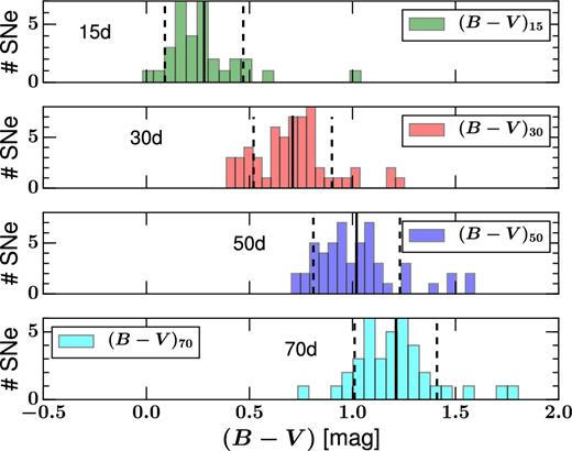
(B − V) colour distributions at four different epochs: 15 d (first from top), 30 d (second from top), 50 d (third from top), and 70 d (bottom) after the explosion. The solid line is the average value while the dashed lines are the 1σ uncertainty.
In Fig. 4, we show how the measured parameters correlate. A strong correlation between the two slopes s1, (B − V) and s2, (B − V) is found with a Pearson factor (r) of 0.60 ± 0.09 (p ≤ 7.7 × 10⁻⁴). This implies that SN II (B − V) colour curves with a slower initial rise also have a slower cooling after transition. Two other trends are also observed between s1, (B − V)/Ttrans, (B − V) and s2, (B − V)/Ttrans, (B − V) with a Pearson factor of −0.39 ± 0.16 (p ≤ 0.15) and −0.36 ± 0.18 (p ≤ 0.27), respectively. This suggests that SN II (B − V) colour curves with a faster evolution (steeper s1, (B − V) or s2, (B − V)) also have a transition at earlier epochs, although at low statistical significance.
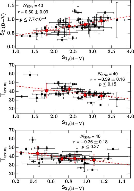
Correlations between the three measured parameters of the SN II (B − V) colour curves. Top: s1, (B − V) with s2, (B − V), both expressed in mag 100d−1. Middle: s1, (B − V) with Ttrans, (B − V) (in days). Bottom: s2, (B − V) with Ttrans, (B − V). In each panel, the number of SNe is listed, together with the Pearson factor and the p-value (p), which indicates the probability of an uncorrelated system producing data sets that have a Pearson factor at least as extreme as the one computed from these data sets.
We also search for correlation between these three (B − V) colour parameters and the colour at four different epochs: 15, 30, 50, and 70 d after the explosion. A slight anticorrelation between Ttrans, (B − V) and the colour (B − V) at 15 d (r = −0.53 ± 0.14, p ≤ 0.11) is seen: bluer SNe II at early epochs have an earlier transition. However, this is not statistically seen at later epochs (30, 50, and 70 d). Finally, as expected, the colours at different epochs correlate strongly: bluer SNe II at 15 d are also bluer at 70 d.
3.3 Photometric/spectroscopic correlations
In this section, we investigate correlations between the (B − V) colour-curve parameters defined in Section 3.1 with spectroscopic (Gutiérrez et al. 2017b) and photometric parameters (Gutiérrez et al. 2017b).
3.3.1 Photometric parameters
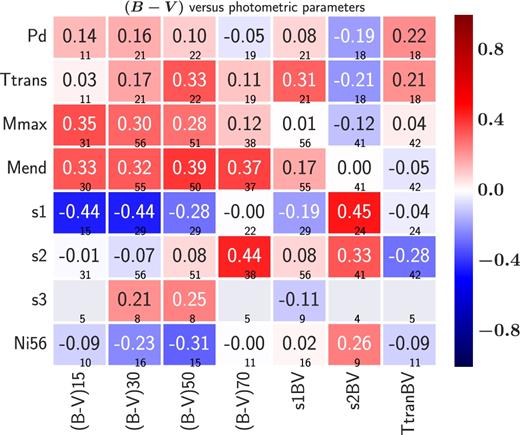
We use a selection of eight photometric parameters discussed by Gutiérrez et al. (2017b): plateau duration (Pd); transition between s1/s2 (Ttrans); absolute V-band magnitude at maximum brightness (Mmax); absolute V-band magnitude measured 30 d before tPT (Mend), where tPT is the midpoint of the transition from plateau to radioactive tail; decline rate of the initial slope of the V-band light curve (s1); slope of the plateau phase (s2); slope of the radiative tail (s3); and 56Ni mass including lower limits (56Ni; see Anderson et al. 2014 for more details). In Fig. 5, the correlation matrix between these photometric parameters and the (B − V) colour-curve parameters defined above is displayed. From this figure, the following trends emerge:
(B − V) at both 15 and 30 d shows some (low significance) correlations with the absolute magnitude, Mmax (respectively, r = 0.35 ± 0.16, p ≤ 0.31; r = 0.30 ± 0.16, p ≤ 0.30) and Mend (respectively, r = 0.33 ± 0.18, p ≤ 0.43; r = 0.32 ± 0.17, p ≤ 0.27): more luminous SNe II are generally bluer (Fig. A3). The later epochs (50–70 d) also correlate with the absolute magnitude, but mainly with Mend (respectively, r = 0.39 ± 0.08, p ≤ 2.8 × 10⁻²; r = 0.37 ± 0.17, p ≤ 0.23). The correlations between the colour at early epochs and the absolute magnitude at maximum brightness could be caused by dust effects (redder SNe II are fainter); however, the strength of this relationship decreases at later epochs (50 and 70d), suggesting that it is driven by intrinsic SN colour differences rather than uncorrected extinction. This is also supported by the analysis presented in Section 5, where we show that the strength of these correlations increases when one removes SNe most likely suffering from significant host-galaxy reddening. Diagrams presenting these magnitude–colour trends are found in Fig. A3.
(B − V) at 30 d and s1 anticorrelate (r = −0.45 ± 0.17, p ≤ 9.9 × 10⁻²) in the sense that bluer SNe II at early epochs show a steeper decline in the V-band after maximum brightness (Fig. A4).
(B − V) at 70 d and s2 correlate (r = 0.44 ± 0.07, p ≤ 2.2 × 10⁻²) in the sense that redder SNe II at later epochs have a steeper plateau slope; they are fast-declining SNe II (Fig. A4).
The matrix correlation between the seven parameters measured from the SN II (B − V) colour curves (B − V at 15, 30, 50, 70 d; s1, (B − V); s2, (B − V); Ttrans, (B-V)) versus the V-band light-curve parameters presented by Gutiérrez et al. (2017b). For each pair, the Pearson factor and the size of the sample are given. The colour bar represents the strength of the relationship. Note that a larger negative number indicates a stronger anticorrelation, while a larger positive number indicates a stronger correlation.
From this analysis, we conclude that low-luminosity SNe II are on average redder and that the colours are dominated by intrinsic differences, since (in addition to the above arguments) the degree of host-galaxy extinction is unlikely to correlate with the decline rates (s1 and s2).
3.3.2 Spectroscopic parameters
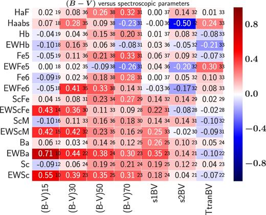
In Fig. 6, the correlation matrix between our 7 parameters derived from the (B − V) colour curves and 16 spectroscopic parameters from Gutiérrez et al. (2017b) is displayed. We used the following spectroscopic parameters: Hα λ6563 velocity obtained from the full width at half-maximum intensity of the emission line (HaF), equivalent width of the H α absorption (Haabs), H β λ4861 velocity (Hb), H β equivalent width (EWHb), and the velocity (measured from the absorption minimum) and the equivalent width of various lines: Fe ii λ5018 (Fe5), Fe ii λ5169 (Fe6), Sc ii/Fe ii λ5531 (ScFe), Sc ii multiplet λ5663 (ScM), Ba ii λ6142 (Ba), and Sc ii λ6247 (Sc). All of the velocities and equivalent widths are measured at 50 d. Fig. 7 shows an example of a SN II spectrum (SN 2005J) at ∼65 d after the explosion with all the used lines and the different filters displayed. In this analysis, we only include equivalent-width measurements when each specific line is detected (i.e. we do not include non-detections). From this figure, the following trends are of interest:
(B − V) colour at different epochs correlates with the equivalent width of different elements. These trends are expected given that metal-line strengths are strongly dependent on the temperature of the line-forming region. At early times (15d), the (B − V) colour correlates with EWBa (r = 0.71 ± 0.07, p ≤ 5.1 × 10⁻²), and slightly with EWSc (r = 0.54 ± 0.19, p ≤ 0.31). Later, at 30 d, the colours appear to correlate with EWBa (r = 0.44 ± 0.11, p ≤ 0.13), EWScM (r = 0.42 ± 0.14, p ≤ 0.11), and EWFe6 (r = 0.41 ± 0.15, p ≤ 0.13), while still later (50 d) only a trend with EWBa (r = 0.38 ± 0.19, p ≤ 0.37) is seen. All of the correlations are plotted in Fig. A5 and indicate that redder SNe II have stronger metal-line equivalent widths.
s2, (B − V) anticorrelates with the strength of the H α absorption line (Haabs) in the sense that SNe II with a rapid cooling after transition exhibit a weaker H α absorption line: r = −0.50 ± 0.07 and p ≤ 1.4 × 10⁻² (Fig. A6).
No statistically significant evidence for a linear relation between the colour and the different velocities is seen.
The correlation matrix between the seven parameters measured from the SN II (B − V) colour curves (B − V at 15, 30, 50, 70 d; s1, (B − V), s2, (B − V), Ttrans, (B − V)) versus the spectroscopic parameters presented by Gutiérrez et al. (2017b). For each pair, the Pearson factor and the size of the sample are given. The colour bar represents the strength of the relationship.
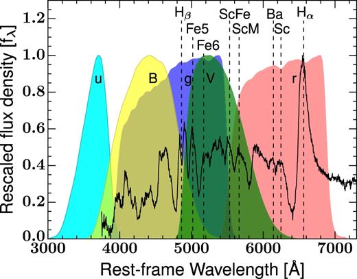
SN 2005J spectrum at 65 d after the explosion. The rest-frame wavelengths (not the absorption minima) of H α λ6563, H β λ4861, Fe ii λ5018 (Fe5), Fe ii λ5169 (Fe6), Sc ii/Fe ii λ5531 (ScFe), Sc ii multiplet λ5663 (ScM), Ba ii λ6142 (Ba), and Sc ii λ6247 (Sc) are marked with dashed lines. Optical filter transmission curves (u, B, g, V, and r) are, respectively, shown in cyan, yellow, blue, green, and red.
4 (u − g), (g − r), AND (g − Y) COLOUR CURVES
In this section, we analyse three others colour curves [(u − g), (g − r), and (g − Y)] and investigate the same trends as previously presented using (B − V). The colour selection was motivated by the aim of studying the possible relation between the metallicity and the colour, H α line effects, and one colour that takes advantage of the NIR. We use only Sloan filters (+Y), as this is currently the most widely adopted photometric system and future projects such as the Large Synoptic Survey Telescope will use similar filters. For the three colours, the procedure used in Section 3 is followed; nevertheless, we do not show all of the figures here, displaying some of them in the Appendix A. Note also that for the three colours, various examples of colour fitting are displayed in Fig. A1.
4.1 (u − g)
4.1.1 Distributions
The parameters measured from (u − g) colour curves have a median s1, (u − g) value of 6.66 ± 2.14 mag 100 d−1, followed by a second slope with a median s2, (u − g) value of 2.53 ± 1.08 mag −1, and a transition Ttrans, (u − g) at 35.3 ± 4.7 d after the explosion. As expected, the slopes s1, (u − g) and s2, (u − g) are steeper than those found with (B − V). This is clearly due to the combination of the temperature (cooling with time) and the strongest sensitivity of the bluest bands to temperature changes. The effect is also seen in observed SN II light curves, where the u band exhibits a faster decline than the other bands (Galbany et al. 2016), as well in theoretical models (Kasen & Woosley 2009; Dessart et al. 2013). Note also, in our SN II sample, only 17 SNe II have u-band data at later epochs, and thus for only 17 SNe II is s2, (u − g) measured.
Regarding the correlations between the two colour-curve parameters (as for (B − V)), s1, (u − g) correlates with s2, (u − g) with a Pearson factor of 0.70 ± 0.11 (p ≤ 1.3 × 10⁻²), and trends are found between s1, (u − g)/Ttrans, (u − g) and s2, (u − g)/Ttrans, (u − g) with respective coefficients of −0.49 ± 0.18 (p ≤ 0.22) and −0.34 ± 0.22 (p ≤ 0.65). Although these trends are weaker than those derived for (B − V) (Section 3.2), they are consistent, confirming that SNe II with a slower initial rise/cooling in their colour curves also show a slower cooling after the transition. These correlations are depicted in Fig. A2.
As for the (B − V) colour, we find an anticorrelation between Ttrans, (u − g) and (u − g) at 15 d, but the number of SNe II is small (r = −0.67 ± 0.17, p ≤ 0.25 for 7 SNe II). Finally, the (u − g) colour distributions at four epochs evolve faster than (B − V) as they become quickly redder with time: <(u − g)15 > =0.49 ± 0.27 mag, <(u − g)30 > =1.53 ± 0.35 mag, <(u − g)50 > =2.36 ± 0.29 mag, and <(u − g)70 > =2.79 ± 0.31 mag at epochs 15, 30, 50, and 70 d, respectively.
4.1.2 Photometric correlations
The relationships found earlier between the absolute magnitude at maximum brightness (Mmax) and the colours are also seen using the (u − g) colour. However, this correlation is only apparent at epoch 30 d (Fig. 8): r = 0.51 ± 0.12 (p ≤ 2.0 × 10⁻²). A trend is also seen for this colour and Mend (r = 0.36 ± 0.25, p ≤ 0.43, Fig. A3), while at the other epochs trends are weak or non-existent.

Correlation between the absolute magnitude at maximum (Mmax) and the (u − g) colour at epoch 30 d. The results of Monte Carlo simulations on the statistics of these two variables are noted at the top of the figure: NSNe (number of events), r (Pearson's correlation coefficient), and p (probability of detecting a correlation by chance). Binned data are shown in red circles, both here and throughout the paper.
We also recover the anticorrelation found previously between the colour at 30 d with s1: r = −0.42 ± 0.15, p ≤ 0.21 (Fig. A4). Regarding the correlation found with (B − V) between the colour at 70 d and s2, here our analysis is restricted by the low number of available events (N = 7).
4.1.3 Spectroscopic correlations
The comparison between (u − g) colours and spectroscopic parameters may reveal interesting trends, given that u-band observations are known to be strongly affected by line-blanketing effects.
The (u − g) colour also correlates with the equivalent width of various elements at different epochs. The correlations seen are on average stronger than for the (B − V) colour. At 15 d with EWScM (r = 0.57 ± 0.15, p ≤ 0.13); at 30 d with EWFe6 (r = 0.53 ± 0.18, p ≤ 7.9 × 10⁻²), EWScFe (r = 0.49 ± 0.15, p ≤ 0.12), and EWScM (r = 0.48 ± 0.12, p ≤ 8.3 × 10⁻²); at 50d with the same elements but weaker, EWFe6 (r = 0.42 ± 0.17, p ≤ 0.25), EWScFe (r = 0.40 ± 0.14, p ≤ 0.25), and EWScM (r = 0.40 ± 0.19, p ≤ 0.34). At later epochs (70 d), the number of SNe is too low to enable any clear conclusions. Specific correlations are shown in Fig. A5.
We find that s1, (u − g) seems to correlate with different equivalent widths such as EwFe5, EWScM, EWBa, and EWScM. However, in each case, the uncertainty in the Pearson coefficient is high, and thus the p-value derived from the upper limit is also high. For example, for EWScFe we have r = 0.43 ± 0.21 (p ≤ 0.26), and for EWBa we have r = 0.35 ± 0.34 (p ≤ 0.97). For all these correlations, the low-luminosity SN 2008bk seems to be an outlier. If we remove this SN, for example in the EWBa relationship, the Pearson factor increases to r = 0.73 ± 0.12 with a very low p-value of p ≤ 9.3 × 10⁻³. This suggests that SNe II with faster initial cooling have larger absorption-line equivalent widths.
4.2 (g − r)
4.2.1 Distributions
The (g − r) colour curves are characterized by an initial slope (s1, (g − r)) with a median value of 1.90 ± 0.53 mag 100 d−1 lasting 37.9 ± 4.3 d (Ttrans, (g − r)), followed by a second slope with a median s2, (g − r) of 0.68 ± 0.25 mag 100 d−1. As for the previous colours, a strong correlation between s1, (g − r) and s2, (g − r) is found (r = 0.43 ± 0.11, p ≤ 4.7 × 10⁻²), and a weaker anticorrelation between s1, (g − r) and Ttrans, (g − r) (r = −0.37 ± 0.17, p ≤ 0.22) is also visible. Again, for (g − r) colour curves, the SNe II with a slow initial rise/cooling also show a slower cooling after the transition that appears at later epochs. Between s2, (g − r) and Ttrans, (g − r), we do not find a correlation (r = −0.07 ± 0.20, p ≤ 0.99).
With this colour, we do not recover previous correlations between Ttrans, (g − r) and the (g − r) colour at 15 d, but one between (g − r) at 70 d and s2, (g − r) is seen (r = 0.45 ± 0.10, p ≤ 3.3 × 10⁻²). Finally, at the same epoch, a correlation with s1, (g − r) (r = 0.52 ± 0.07, p ≤ 5.2 × 10⁻³) is also seen. Redder SNe II at late epochs have a faster cooling before and after the transition in their colour curves. However, it is important to note that these two correlations are seen only using (g − r).
We also look at the (g − r) colour distributions at four epochs. As expected, (g − r) becomes redder with time: <(g − r)15 > =0.24 ± 0.28 mag, <(g − r)30 > =0.55 ± 0.25 mag, <(g − r)50 > =0.79 ± 0.21 mag, and <(g − r)70 > =0.94 ± 0.24 mag at epochs 15, 30, 50, and 70 d, respectively. The colour evolution is much slower than for (u − g) or (B − V), as the shape of the red part of the spectrum is less affected by the temperature change during the photospheric phase.
4.2.2 Photometric correlations
We recover the correlations between the colour and the absolute magnitude found with (B − V) and (u − g): (g − r) at 15 and 30 d with the absolute magnitude Mmax (respectively, r = 0.53 ± 0.11, p ≤ 1.5 × 10⁻²; r = 0.38 ± 0.17, p ≤ 0.11) or Mend (respectively, r = 0.58 ± 0.11, p ≤ 6.6 × 10⁻³; r = 0.48 ± 0.12, p ≤ 5.0 × 10⁻³); see Fig. A3. In these diagrams, the outlier is SN 2008bp, which was also identified as an outlier by Anderson et al. (2014). Finally, the absence of correlation at later epochs (50 and 70 d) suggests an intrinsic origin rather than dust extinction.
For this colour, two relations found previously are also seen. First, the colour at later epochs correlates with s2. A weak correlation is seen at 50 d (r = 0.33 ± 0.19, p ≤ 0.32), which becomes stronger 20 d later (r = 0.64 ± 0.004, p ≤ 7.0 × 10⁻⁶). This correlation means that redder SNe II at later epochs have a steeper plateau decline rate (see Fig. A4). Secondly, the anticorrelation between the colour at early epochs and s1 is also found (r = −0.60 ± 0.05, p ≤ 2.7 × 10⁻²): bluer SNe II have a steeper initial decline — they are fast-declining SNe II (Fig. 10).
4.2.3 Spectroscopic correlations
The (g − r) colour at 30 d also correlates slightly or strongly with different equivalent widths such as Haabs (r = 0.48 ± 0.19, p ≤ 0.49) or EWFe6 (r = 0.48 ± 0.05, p ≤ 9.9 × 10⁻³), in the sense that bluer SNe II have smaller equivalent widths. Note also that (g − r) at 50 d correlates with EWFe6 (r = 0.45 ± 0.08, p ≤ 1.9 × 10⁻²). These correlations are shown in Fig. A5.
We also see a weak anticorrelation between the strength of the H α absorption line (Haabs) and s2, (g − r) in the sense that SNe II with a rapid cooling after transition show a weaker H α absorption line: r = −0.41 ± 0.16 and p ≤ 0.15 (Fig. A6).
Even if these correlations are not seen for the previous colours, we think it is important to mention that (g − r) at 50 and 70 d correlate with different velocities in the sense that redder SNe II at later epochs have faster velocities: HaF (respectively, r = 0.51 ± 0.03, p ≤ 1.7 × 10⁻³; r = 0.58 ± 0.02, p ≤ 5.7 × 10⁻⁴), Hb (respectively, r = 0.42 ± 0.09, p ≤ 3.7 × 10⁻²; r = 0.50 ± 0.05, p ≤ 7.5 × 10⁻³), Fe5 (respectively, r = 0.48 ± 0.06, p ≤ 7.0 × 10⁻³; r = 0.59 ± 0.03, p ≤ 5.7 × 10⁻⁴), ScFe (respectively, r = 0.49 ± 0.04, p ≤ 5.9 × 10⁻³; r = 0.60 ± 0.02, p ≤ 5.0 × 10⁻⁴), ScM (respectively, r = 0.44 ± 0.08, p ≤ 2.6 × 10⁻²; r = 0.47 ± 0.09, p ≤ 2.9 × 10⁻²), and Sc (respectively, r = 0.50 ± 0.09, p ≤ 3.3 × 10⁻²; r = 0.60 ± 0.07, p ≤ 6.4 × 10⁻³). The correlations are displayed in Fig. A7.
Finally, it is also important to note that (g − r) correlates better with the spectroscopic parameters derived from the H α line than (B − V) or (u − g). This is not surprising, as in the rest frame the H α line falls directly inside the r filter (effective wavelength λ6223.3; see http://csp.obs.carnegiescience.edu/data/filters).
4.3 (g − Y)
4.3.1 Distributions
The (g − Y) colour curves are characterized by an initial cooling (s1, (g − Y)) with a median value of 2.95 ± 0.49 mag 100 d−1 followed by a second slope with a median s2, (g − Y) of 0.83 ± 0.31 mag 100 d−1, and a transition Ttrans, (g − Y) at 39.6 ± 4.3 d after the explosion.
While for the other colours, strong correlations between the two colour slopes are seen (see Fig. A2), for (g − Y) no statistically significant trend is found (r = 0.19 ± 0.18, p ≤ 0.97). Additionally, the anticorrelation between s1, (g − Y)/Ttrans, (g − Y) is weak, with r = −0.49 ± 0.21 (p ≤ 0.23), while the one between s2, (g − Y)/Ttrans, (g − Y) is strong, with r = −0.55 ± 0.12 (p ≤ 5.8 × 10⁻²). We also try to correlate these three parameters with the colours at four different epochs as achieved in the previous sections. No correlations were found as for the previous colour sets.
Repeating our previous analysis, we look at the (g − Y) colour distributions at four epochs. We find that (g − Y) becomes redder with time: <(g − Y)15 > = 0.49 ± 0.37 mag, <(g − Y)30 > = 1.01 ± 0.31 mag, <(g − Y)50 > = 1.43 ± 0.43 mag, and <(g − Y)70 > = 1.62 ± 0.44 mag at epoch 15, 30, 50, and 70 d, respectively. At early times (15 d), the statistics are very low, with only 14 SNe II (versus 37, 37, and 25 SNe II for 30, 50, and 70 d, respectively).
4.3.2 Photometric correlations
As for other colour combinations, we find that more luminous SNe II are bluer. Although only a weak trend is seen with Mmax, with Mend the correlation is stronger at different epochs. The correlation factors are r = 0.66 ± 0.14 (p ≤ 6.8 × 10⁻²), r = 0.41 ± 0.11 (p ≤ 4.1 × 10⁻²), and r = 0.48 ± 0.13 (p ≤ 3.1 × 10⁻²) for 15, 30, and 50 d, respectively (Fig. A3).
Regarding the other photometric correlations seen in the previous sections; here, we only recover the correlation between (g − Y) at 70 d and s2 (r = 0.50 ± 0.06, p ≤ 6.1 × 10⁻²) – that is, redder SNe II have steeper s2 (Fig. A4).
4.3.3 Spectroscopic correlations
For the (g − Y) colour, only one slight correlation between the colour at 30 d and the equivalent width EWFe6 is seen (Fig. A5), in the sense that redder SNe II show larger equivalent widths (r = 0.41 ± 0.11, p ≤ 0.12). However, we do not recover the correlation between s2, (g − Y) and Haabs. Finally, note that as with (g − r), a correlation between the velocities and the colours at late epochs (50 and 70 d) is seen: redder SNe II at late epochs have faster ejecta velocities.
5 HOST-GALAXY EXTINCTION EFFECTS
5.1 Colour-brightness correlations
As mentioned previously, in this work we do not correct for host-galaxy extinction, as no currently available method seems to improve the uniformity of the SN II sample (Faran et al. 2014a; Gutiérrez et al. 2017b). However, here we discuss the possible effects of host-galaxy extinction on the colour–brightness correlations. For this purpose, we use three different subsamples as well as the full sample.
Comparison of correlation strengths between colours and absolute magnitudes.
| Correlations | All sample | Sample cut | Sample cut | Sample cut | ||||||||
|---|---|---|---|---|---|---|---|---|---|---|---|---|
| based on colours | based on Na i D | based on Na i D + position | ||||||||||
| NSNe | r | p ≤ | NSNe | r | p ≤ | NSNe | r | p ≤ | NSNe | r | p ≤ | |
| (B − V)15 versus Mmax | 31 | 0.35 ± 0.16 | 0.31 | 28 | 0.50 ± 0.10 | 3.5 × 10⁻² | 22 | 0.49 ± 0.10 | 7.3 × 10⁻² | 12 | 0.49 ± 0.22 | 0.40 |
| (B − V)15 versus Mend | 30 | 0.33 ± 0.18 | 0.43 | 27 | 0.44 ± 0.14 | 0.13 | 21 | 0.49 ± 0.09 | 7.2 × 10⁻² | 12 | 0.59 ± 0.18 | 0.19 |
| (B − V)30 versus Mmax | 56 | 0.30 ± 0.16 | 0.30 | 50 | 0.47 ± 0.03 | 1.4 × 10⁻³ | 36 | 0.39 ± 0.14 | 0.14 | 18 | 0.30 ± 0.27 | 0.92 |
| (B − V)30 versus Mend | 55 | 0.32 ± 0.17 | 0.27 | 49 | 0.40 ± 0.13 | 6.1 × 10⁻² | 35 | 0.35 ± 0.19 | 0.36 | 18 | 0.24 ± 0.29 | 0.83 |
| (B − V)50 versus Mend | 50 | 0.39 ± 0.08 | 2.8 × 10⁻² | 45 | 0.33 ± 0.16 | 0.26 | 30 | 0.34 ± 0.21 | 0.49 | 15 | 0.42 ± 0.26 | 0.57 |
| (B − V)70 versus Mend | 37 | 0.37 ± 0.17 | 0.23 | 33 | 0.23 ± 0.29 | 0.74 | 24 | 0.10 ± 0.30 | 0.35 | 11 | 0.34 ± 0.31 | 0.92 |
| (u − g)30 versus Mmax | 35 | 0.51 ± 0.12 | 2.0 × 10⁻³ | 31 | 0.56 ± 0.03 | 2.1 × 10⁻³ | 26 | 0.54 ± 0.06 | 1.3 × 10⁻² | 12 | 0.39 ± 0.22 | 0.59 |
| (u − g)30 versus Mend | 34 | 0.36 ± 0.22 | 0.43 | 31 | 0.41 ± 0.24 | 0.36 | 25 | 0.49 ± 0.12 | 6.9 × 10⁻² | 12 | 0.25 ± 0.31 | 0.86 |
| (g − r)15 versus Mmax | 33 | 0.53 ± 0.11 | 1.5 × 10⁻³ | 30 | 0.57 ± 0.03 | 2.1 × 10⁻³ | 23 | 0.69 ± 0.01 | 3.6 × 10⁻⁴ | 12 | 0.52 ± 0.19 | 0.29 |
| (g − r)15 versus Mend | 32 | 0.58 ± 0.11 | 6.6 × 10⁻³ | 29 | 0.46 ± 0.14 | 9.0 × 10⁻² | 22 | 0.77 ± 0.02 | 5.8 × 10⁻⁵ | 12 | 0.43 ± 0.27 | 0.62 |
| (g − r)30 versus Mmax | 57 | 0.38 ± 0.17 | 0.11 | 51 | 0.34 ± 0.11 | 0.10 | 37 | 0.47 ± 0.16 | 6.2 × 10⁻² | 18 | 0.18 ± 0.28 | 0.69 |
| (g − r)30 versus Mend | 56 | 0.49 ± 0.12 | 5.0 × 10⁻³ | 50 | 0.36 ± 0.16 | 0.16 | 36 | 0.55 ± 0.18 | 2.6 × 10⁻² | 18 | 0.08 ± 0.27 | 0.44 |
| (g − Y)15 versus Mend | 13 | 0.66 ± 0.14 | 6.8 × 10⁻³ | 12 | 0.73 ± 0.09 | 3.1 × 10⁻² | 8 | 0.59 ± 0.21 | 0.35 | 5 | ⋅⋅⋅ ± ⋅⋅⋅ | ⋅⋅⋅ |
| (g − Y)30 versus Mend | 39 | 0.41 ± 0.11 | 6.3 × 10⁻³ | 35 | 0.54 ± 0.02 | 1.4 × 10⁻³ | 25 | 0.27 ± 0.26 | 0.96 | 14 | 0.25 ± 0.30 | 0.88 |
| (g − Y)50 versus Mend | 38 | 0.48 ± 0.13 | 3.1 × 10⁻² | 34 | 0.30 ± 0.23 | 0.69 | 23 | 0.21 ± 0.29 | 0.72 | 11 | 0.06 ± 0.30 | 0.47 |
Notes. Four different samples are used: total (all), removing 10 per cent of the reddest objects (based on colours), only the SNe II with an Na i D equivalent width smaller than 1 Å (based on Na i D), and only the SNe II away from the host-galaxy nuclei with no Na i D equivalent width (based on Na i D + position).
First, we assume that in those SNe showing the reddest colours, the majority of this colour is dominated by uncorrected host-galaxy extinction. While throughout this article we argue that most of the diversity in SN II colours is intrinsic, it is expected that some SNe II do suffer from considerable host-galaxy extinction, given that galactic environments with a high dust content are known to exist. In this context, for each colour–brightness correlation presented, we remove SNe II that have colours falling within the ∼10 per cent reddest of the sample. For each correlation, the exact colour and the epoch are different, and therefore, the exact colour cut value changes. However, using the (B − V) colour (for example), the cut occurs at ∼0.45, 0.9, 1.3, and 1.4 mag for 15, 30, 50, and 70 d, respectively. In Table 2, a comparison of the correlation strengths without (first column) and with (second column) the colour cut is shown. The strength of correlations generally increased after removing these reddest SNe II, suggesting an intrinsic explanation of the colour-brightness relation (as discussed below). While the choice of 10 per cent was initially arbitrary, we also tested cuts of ∼20 per cent and ∼30 per cent. However, in both of these latter cases the strengths of correlations generally decreased, and thus our choice of 10 per cent appears to be justified.
Secondly, even if the validity of the use of Na i D in low-resolution spectra for deriving precise host-galaxy extinction has been challenged (Poznanski et al. 2011; Phillips et al. 2013; Galbany et al. 2017), the presence of significant Na i D absorption does usually imply some degree of host-galaxy extinction. The absence of this Na i D absorption line also probably indicates a low level of host-galaxy extinction. So, here we remove all SNe II that have an Na i D equivalent width ≥1 Å (Anderson et al. 2014). In the third column of Table 2, the new correlations for this sample are listed; again, we generally find an increase in correlation strength when removing those events most likely to be significantly affected by dust extinction.
Finally, following the procedure of Phillips et al. (1999), Folatelli et al. (2010), and Stritzinger et al. (2018), we choose SNe II that are located at significant distances away from host-galaxy nuclei, together with those that do not have Na i D absorption detections (AV(host) =0.00 from table 6 in Anderson et al. 2014). This final sample consists of 19 SNe II (13 SNe II with NIR photometry). The new correlations are presented in the fourth column of Table 2.
Comparing the strength of correlations in the first two subsamples to those of our full sample, we can assess the likelihood of host-galaxy extinction producing our observed trends. If any of the trends are produced by the effects of uncorrected reddening, one should expect the strength of correlations to decrease in the subsamples where we remove SNe II affected by significant host-galaxy extinction. We see that the majority of the correlations (mostly at earlier epochs) are stronger for the culled samples (colour or Na i D). This confirms our hypothesis of an intrinsic origin for the dominant colour diversity rather that dust effects, in the majority of our sample. Note also that the differences between the full sample and subsamples are generally stronger with Mmax than Mend. Regarding the subsample with both Na i D absorption and position cuts, the statistics are too low to enable meaningful conclusions (although there is no evidence that correlation strengths decrease in this sample); however, this subsample will be useful for investigating the intrinsic colour of our SNe II (Section 6.6).
5.2 Other correlations
Following the procedure from the previous section, we investigate the effect of host-galaxy extinction in all of the correlations found in this work. A summary of the Pearson factor between the full sample and three subsamples (colour, Na i D equivalent width, and Na i D equivalent width + position) are, respectively, displayed in the first, second, third, and fourth columns of Table 3.
Comparison of correlation strengths between colours and spectroscopic/photometric parameters.
| Correlations | All sample | Sample cut | sample cut | sample cut | ||||||||
|---|---|---|---|---|---|---|---|---|---|---|---|---|
| based on colours | based on Na i D | based on Na i D + position | ||||||||||
| NSNe | r | p ≤ | NSNe | r | p ≤ | NSNe | r | p ≤ | NSNe | r | p ≤ | |
| (B − V)70 versus s2 | 38 | 0.44 ± 0.07 | 2.2 × 10⁻² | 34 | 0.33 ± 0.20 | 0.46 | 24 | 0.22 ± 0.28 | 0.78 | 11 | 0.14 ± 0.26 | 0.71 |
| (g − r)50 versus s2 | 53 | 0.33 ± 0.19 | 0.32 | 48 | 0.38 ± 0.12 | 7.4 × 10⁻² | 31 | 0.39 ± 0.15 | 0.19 | 15 | 0.46 ± 0.24 | 0.42 |
| (g − r)70 versus s2 | 41 | 0.64 ± 0.005 | 7.0 × 10⁻⁶ | 37 | 0.60 ± 0.01 | 1.2 × 10⁻⁴ | 25 | 0.61 ± 0.06 | 4.3 × 10⁻³ | 11 | 0.34 ± 0.27 | 0.85 |
| (g − Y)70 versus s2 | 25 | 0.50 ± 0.12 | 6.1 × 10⁻² | 23 | 0.54 ± 0.09 | 3.1 × 10⁻² | 14 | 0.51 ± 0.19 | 0.26 | 6 | 0.40 ± 0.53 | 0.81 |
| (B − V)15 versus s1 | 15 | −0.44 ± 0.23 | 0.45 | 13 | −0.31 ± 0.28 | 0.93 | 12 | −0.41 ± 0.26 | 0.64 | 5 | ⋅⋅⋅ ± ⋅⋅⋅ | ⋅⋅⋅ |
| (B − V)30 versus s1 | 29 | −0.44 ± 0.13 | 9.9 × 10⁻² | 26 | −0.57 ± 0.08 | 1.1 × 10⁻² | 20 | −0.53 ± 0.13 | 8.1 × 10⁻² | 7 | −0.57 ± 0.31 | 0.65 |
| (u − g)30 versus s1 | 23 | −0.42 ± 0.15 | 0.21 | 21 | −0.52 ± 0.10 | 6.5 × 10⁻² | 17 | −0.37 ± 0.22 | 0.56 | 5 | ⋅⋅⋅ ± ⋅⋅⋅ | ⋅⋅⋅ |
| (g − r)15 versus s1 | 16 | −0.60 ± 0.05 | 2.7 × 10⁻² | 14 | −0.58 ± 0.10 | 8.2 × 10⁻² | 13 | −0.57 ± 0.11 | 0.11 5 | ⋅⋅⋅ | ⋅⋅⋅ ± ⋅⋅⋅ | ⋅⋅⋅ |
| (B − V)15 versus EWSc | 10 | 0.55 ± 0.19 | 0.31 | 9 | 0.63 ± 0.19 | 0.24 | 7 | 0.67 ± 0.20 | 0.29 | 7 | 0.73 ± 0.28 | 0.31 |
| (B − V)15 versus EWBa | 10 | 0.71 ± 0.08 | 5.1 × 10⁻² | 9 | 0.62 ± 0.13 | 0.18 | 7 | 0.67 ± 0.16 | 0.24 | 7 | 0.73 ± 0.28 | 0.31 |
| (u − g)15 versus EWScM | 14 | 0.57 ± 0.15 | 0.13 | 13 | 0.62 ± 0.09 | 6.2 × 10⁻² | 5 | ⋅⋅⋅ ± ⋅⋅⋅ | ⋅⋅⋅ | 5 | ⋅⋅⋅ ± ⋅⋅⋅ | ⋅⋅⋅ |
| (B − V)30 versus EWBa | 22 | 0.44 ± 0.11 | 0.13 | 20 | 0.53 ± 0.10 | 5.8 × 10⁻² | 15 | 0.51 ± 0.17 | 0.21 | 11 | 0.28 ± 0.39 | 0.75 |
| (B − V)30 versus EWScM | 32 | 0.42 ± 0.13 | 0.11 | 29 | 0.54 ± 0.04 | 5.7 × 10⁻³ | 22 | 0.43 ± 0.17 | 0.24 | 11 | 0.58 ± 0.17 | 0.11 |
| (B − V)30 versus EWFe6 | 35 | 0.41 ± 0.15 | 0.13 | 31 | 0.30 ± 0.28 | 0.91 | 25 | 0.31 ± 0.28 | 0.89 | 11 | −0.28 ± 0.33 | 0.89 |
| (u − g)30 versus EWFe6 | 26 | 0.53 ± 0.18 | 7.9 × 10⁻² | 23 | 0.39 ± 0.26 | 0.55 | 18 | 0.33 ± 0.28 | 0.84 | 9 | 0.06 ± 0.26 | 0.62 |
| (u − g)30 versus EWScM | 24 | 0.48 ± 0.12 | 8.3 × 10⁻² | 22 | 0.58 ± 0.03 | 8.0 × 10⁻³ | 18 | 0.50± 0.13 | 0.13 | 9 | 0.54 ± 0.26 | 0.46 |
| (u − g)30 versus Haabs | 26 | 0.46 ± 0.16 | 0.14 | 23 | 0.51 ± 0.15 | 9.1 × 10⁻² | 18 | 0.26 ± 0.29 | 0.91 | 9 | 0.28 ± 0.29 | 0.97 |
| (u − g)30 versus EWScFe | 22 | 0.49 ± 0.15 | 0.12 | 20 | 0.61 ± 0.03 | 7.3 × 10⁻³ | 16 | 0.49 ± 0.19 | 0.26 | 9 | 0.79 ± 0.12 | 5.0 × 10⁻² |
| (g − r)30 versus Haabs | 35 | 0.31 ± 0.19 | 0.49 | 31 | 0.41 ± 0.16 | 5.3 × 10⁻² | 25 | 0.30 ± 0.23 | 0.74 | 11 | 0.06 ± 0.35 | 0.40 |
| (g − r)30 versus EWFe6 | 35 | 0.48 ± 0.05 | 9.9 × 10⁻³ | 31 | 0.46 ± 0.14 | 7.9 × 10⁻² | 25 | 0.42 ± 0.21 | 0.31 | 11 | 0.01 ± 0.4 | 0.23 |
| (g − Y)30 versus EWFe6 | 28 | 0.41 ± 0.11 | 0.12 | 25 | 0.32 ± 0.19 | 0.53 | 19 | 0.37 ± 0.28 | 0.71 | 8 | 0.65 ± 0.24 | 0.31 |
| (B − V)50 versus EWBa | 24 | 0.38 ± 0.19 | 0.37 | 22 | 0.65 ± 0.02 | 1.7 × 10⁻³ | 17 | 0.46 ± 0.25 | 0.42 | 13 | 0.39 ± 0.30 | 0.78 |
| (u − g)50 versus EWFe6 | 23 | 0.42 ± 0.17 | 0.25 | 21 | 0.38 ± 0.23 | 0.52 | 18 | 0.33 ± 0.28 | 0.84 | 9 | 0.31 ± 0.27 | 0.91 |
| (u − g)50 versus EWScFe | 21 | 0.40 ± 0.14 | 0.25 | 19 | 0.33 ± 0.23 | 0.68 | 16 | 0.35 ± 0.25 | 0.71 | 9 | 0.67 ± 0.22 | 0.22 |
| (u − g)50 versus EWScM | 23 | 0.40 ± 0.19 | 0.34 | 21 | 0.41 ± 0.23 | 0.43 | 18 | 0.32 ± 0.29 | 0.91 | 9 | 0.30 ± 0.34 | 0.91 |
| (g − r)50 versus EWFe6 | 40 | 0.45 ± 0.08 | 1.9 × 10⁻² | 36 | 0.44 ± 0.07 | 4.2 × 10⁻² | 27 | 0.39 ± 0.20 | 0.34 | 13 | 0.12 ± 0.30 | 0.56 |
| s2, (B − V) versus Haabs | 32 | −0.50 ± 0.07 | 1.4 × 10⁻² | 29 | −0.39 ± 0.18 | 0.27 | 24 | −0.50 ± 0.15 | 9.4 × 10⁻² | 13 | −0.59 ± 0.22 | 0.36 |
| s2, (g − r) versus Haabs | 35 | −0.41 ± 0.16 | 0.15 | 31 | −0.27 ± 0.25 | 0.91 | 24 | −0.59 ± 0.08 | 1.1 × 10⁻² | 12 | −0.56 ± 0.17 | 0.16 |
| (g − r)50 versus HaF | 40 | 0.51 ± 0.03 | 1.5 × 10⁻³ | 36 | 0.46 ± 0.09 | 3.6 × 10⁻² | 27 | 0.40 ± 0.19 | 0.29 | 13 | 0.40 ± 0.22 | 0.57 |
| (g − r)50 versus Hb | 40 | 0.42 ± 0.09 | 3.7 × 10⁻² | 36 | 0.36 ± 0.17 | 0.27 | 27 | 0.32 ± 0.24 | 0.37 | 13 | 0.37 ± 0.24 | 0.66 |
| (g − r)50 versus Fe5 | 40 | 0.48 ± 0.06 | 7.0 × 10⁻³ | 36 | 0.44 ±0.12 | 5.7 × 10⁻² | 27 | 0.41 ±0.19 | 0.27 | 13 | 0.47 ± 0.25 | 0.49 |
| (g − r)50 versus ScFe | 36 | 0.49 ± 0.04 | 5.9 × 10⁻³ | 32 | 0.46 ± 0.10 | 4.3 × 10⁻² | 23 | 0.34 ± 0.24 | 0.65 | 11 | 0.47 ± 0.29 | 0.61 |
| (g − r)50 versus ScM | 38 | 0.44 ± 0.08 | 2.6 × 10⁻² | 34 | 0.39 ± 0.17 | 0.21 | 25 | 0.26 ± 0.27 | 0.97 | 12 | 0.44 ± 0.25 | 0.56 |
| (g − r)50 versus Sc | 27 | 0.50 ± 0.09 | 3.3 × 10⁻² | 24 | 0.46 ± 0.14 | 0.12 | 17 | 0.41 ± 0.23 | 0.49 | 8 | 0.13 ± 0.50 | 0.36 |
| (g − Y)50 versus HaF | 33 | 0.40 ± 0.13 | 0.13 | 30 | 0.36 ± 0.23 | 0.49 | 21 | 0.36 ± 0.28 | 0.73 | 9 | 0.42 ± 0.24 | 0.65 |
| (g − r)70 versus Hb | 34 | 0.50 ± 0.05 | 7.5 × 10⁻³ | 31 | 0.33 ± 0.19 | 0.45 | 22 | 0.38 ± 0.21 | 0.45 | 10 | 0.01 ± 0.43 | 0.86 |
| (g − r)70 versus HaF | 34 | 0.58 ± 0.02 | 5.7 × 10⁻⁴ | 31 | 0.45 ± 0.10 | 5.3 × 10⁻² | 22 | 0.44 ± 0.16 | 0.21 | 10 | 0.07 ± 0.44 | 0.30 |
| (g − r)70 versus Fe5 | 34 | 0.59 ± 0.03 | 5.7 × 10⁻⁴ | 31 | 0.39 ± 0.15 | 0.19 | 22 | 0.44 ± 0.18 | 0.24 | 10 | 0.08 ± 0.45 | 0.28 |
| (g − r)70 versus ScFe | 32 | 0.60 ± 0.02 | 5.0 × 10⁻⁴ | 29 | 0.45 ± 0.08 | 4.8 × 10⁻² | 20 | 0.42 ± 0.17 | 0.29 | 9 | 0.15 ± 0.48 | 0.38 |
| (g − r)70 versus ScM | 33 | 0.47 ± 0.09 | 2.9 × 10⁻² | 30 | 0.29 ± 0.24 | 0.80 | 21 | 0.26 ± 0.28 | 0.93 | 9 | 0.01 ± 0.53 | 0.25 |
| (g − r)70 versus Sc | 25 | 0.60 ± 0.07 | 6.4 × 10⁻³ | 23 | 0.41 ± 0.16 | 0.25 | 16 | 0.43 ± 0.21 | 0.41 | 7 | −0.29 ± 0.43 | 0.82 |
| (g − Y)70 versus HaF | 21 | 0.52 ± 0.18 | 0.13 | 19 | 0.35 ± 0.28 | 0.77 | 13 | 0.48 ± 0.26 | 0.47 | 5 | ⋅⋅⋅ ± ⋅⋅⋅ | ⋅⋅⋅ |
| (g − Y)70 versus Hb | 21 | 0.44 ± 0.17 | 0.24 | 19 | 0.28 ± 0.30 | 0.93 | 13 | 0.40 ± 0.28 | 0.70 | 5 | ⋅⋅⋅ ± ⋅⋅⋅ | ⋅⋅⋅ |
| (g − Y)70 versus Fe5 | 21 | 0.55 ± 0.14 | 6.5 × 10⁻² | 19 | 0.43 ± 0.24 | 0.44 | 13 | 0.58 ± 0.20 | 0.20 | 5 | ⋅⋅⋅ ± ⋅⋅⋅ | ⋅⋅⋅ |
Notes. Four different samples are used: total (all), removing 10 per cent of the reddest objects (based on colours), only the SNe II with an Na i D equivalent width smaller than 1 Å (based on Na i D), and only the SNe II away from the host-galaxy nuclei with no Na i D equivalent width (based on Na i D + position).
This analysis provides additional support for our conclusion that the correlations are driven mostly by intrinsic origin, as in the majority of the cases the Pearson factor is stronger for the subsamples than for the full sample. Note that the strength increase is more likely seen at earlier epochs (15–30 d) than at later epochs (50–70 d). This could explain why the strengths of the colour/velocity correlations are not greater for the culled sample, as these correlations are only seen at later epochs.
6 DISCUSSION
Using 65 SNe II from the CSP-I sample, four different colours (B − V, u − g, g − r, and g − Y) and their evolution have been characterized. We define morphological colour-curve parameters, measure observed colours at different phases, and explore possible correlations between colour parameters and different spectroscopic and photometric properties. We now discuss these results in more detail, and we compare them to other observational and theoretical SN II studies.
6.1 Colour evolution
First, using a larger SN II sample than that of Patat et al. (1994), we confirm their finding that SN II colour curves consist of two regimes with two different slopes (see Fig. 1 and Section A1). While a linear fit (one or two slopes) describes the majority of SN II colour curves better than a power-law fit (55 per cent for B − V or 63 per cent for g − r), it is important to note that for the (g − Y) colour, half of the SN II light curves favour a power-law fit (51 per cent). For this colour, only a very small fraction is described by two slopes, even if the SN colour curve is well sampled. Finally, for the (u − g) colour, the majority of the SN II colour curves are fitted by only one slope (54 per cent); however, this can be explained by the lack of u-band data at late epochs.
Secondly, the study of colour-curve parameters with four different colours leads to the overall conclusion that SNe II which cool more quickly at early epochs also generally cool more quickly during the plateau phase. This correlation between s1, colour and s2, colour is clearly seen in Fig. 4 with a Pearson factor of 0.60 ± 0.09 (p ≤ 7.7 × 10⁻⁴). This correlation is also found for (u − g) and (g − r); however, for (g − Y), the correlation is not statistically significant (see Fig. A2).
Some trends are also observed between the epoch of the transition in the colour curve and the decline rate of the two slopes. While the trends are not statistically significant for all colours, in general SNe II which cool faster (at both early and later times) have a transition at earlier epochs (see Figs 4 and A2). It is possible that this can be understood in terms of the effects of additional energy (beyond the shock-deposited energy from the core-collapse explosion) from interaction with CSM close to the progenitor star (e.g. Khazov et al. 2016; Morozova et al. 2016; Dessart et al. 2017; Moriya et al. 2017; Morozova et al. 2017; Yaron et al. 2017). Such interaction may slow the colour evolution, keeping the photosphere bluer for longer and in effect stretching the colour evolution in time.
Finally, the colours at early and late epochs correlate in the sense that bluer SNe II at 15 d are generally also bluer at 70 d. For example, (B − V) at 15 d correlates with (B − V) at 30, 50, and 70 d with a Pearson factor of 0.85 ± 0.01 (p ≤ 1.0 × 10⁻⁶), 0.77 ± 0.02 (p ≤ 1.0 × 10⁻⁵), and 0.79 ± 0.02 (p ≤ 7.8 × 10⁻⁴), respectively. The same trend is also seen for (u − g), (g − r), and (g − Y). If early-time colour differences are expected (in part) to be caused by differences in progenitor radii (e.g. Dessart et al. 2013), then one would not expect to see this result. Differences in progenitor radii are expected to affect the time taken for photospheric temperatures to reach those of hydrogen recombination (and thus the early-time colours and the transition between the different phases, although see Faran et al. 2018); however, one would then expect temperatures – and therefore colours – to converge to those required for hydrogen recombination. The correlation between colours at early and late photospheric epochs could then be understood either through the continued effect of CSM interaction, or the constant colour excess expected from any uncorrected host-galaxy reddening.4
6.2 Are redder SNe II fainter?
For each colour combination at early epochs (15–30 d), redder SNe II appear to be less luminous than bluer SNe II. As an example, in Fig. 8, the (u − g) colour at epoch 30 d and the absolute magnitude at maximum brightness are shown. This statement is not a new result for the SN community, as it has already been shown for SNe Ia in a number of papers starting more than two decades ago (e.g. Hamuy et al. 1996; Riess et al. 1996; Tripp 1998) and fully used for SN standardization. However, to our knowledge, this is the first time that a study of SNe II presents such correlations using different colours, epochs, and with a large sample (Section A3). Also, note that the (B − V) colour comparison between our large SN II luminosity distribution and literature low-luminosity SNe II leads to the same conclusion. At an epoch of 60 d after explosion, Spiro et al. (2014) derived a mean value of (B − V) ≈ 1.4 mag for a sample of low-luminosity SNe II [(B − V) ≈ 1.5 mag found by Pastorello et al. 2004. Using our sample of normal SNe II, at this epoch we derive a smaller value [(B − V) = 1.10 ± 0.18 mag], thus confirming that redder SNe II are intrinsically fainter. (It is important to note here that the literature low-luminosity sample was corrected for host-galaxy extinction.)
This correlation could be a direct effect of dust extinction that would make SNe both redder and fainter. Studies that have assumed such a hypothesis have concluded that the dust properties in SN host galaxies are incompatible with those in the MW (Krisciunas et al. 2007; Elias-Rosa et al. 2008; Goobar 2008; Poznanski et al. 2009; Folatelli et al. 2010; Olivares et al. 2010; Phillips et al. 2013; Rodríguez et al. 2014; de Jaeger et al. 2015). One possible explanation is the existence of an additional intrinsic relationship between SN colour and luminosity.
Our results can be used to argue for an intrinsic origin of this luminosity versus colour relation. At early epochs (15–30 d), the correlation between colour and Mmax is stronger than at late epochs (50–70 d). For example, the (g − r) colour at 15 d correlates with Mmax (r ≈ 0.53), but not at 50 d (r ≈ 0.04). For (B − V), the same is seen, with a Pearson factor at 15 d of ∼0.35 but only r ≈ 0.28 and r ≈ 0.12 at 50 and 70 d, respectively. If the luminosity versus colour relations were driven by reddening from dust, one would not expect to see such differences, thus arguing for an intrinsic origin. This is also supported by our tests regarding the specific effects of host-galaxy extinction on our results (see Section 5): if we remove those SNe II that we expect to suffer from significant host-galaxy reddening, the correlations between the colour and Mmax generally become stronger (see Table 2) instead of weaker. An additional argument in favour of an intrinsic origin is that if all the colour diversity were simply due to extinction, then one would not expect to see any correlation with other parameters not affected by extinction, such as s2. However, the colour at late times clearly correlates with s2 (Fig. 9).
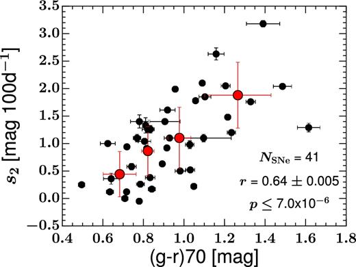
Correlation between the slope of the plateau (s2) in the V band and the (g − r) colour at epoch 70 d. The results of Monte Carlo simulations on the statistics of these two variables are noted at the bottom of the figure in a similar way to Fig. 4.
In conclusion, there is strong evidence that brighter SNe II are also bluer during the first few weeks after explosion. Such a result can be naturally explained through progenitor radii differences: SNe II with more compact progenitors cool more quickly through rapid expansion. At the same time, in such compact progenitors significant internal energy is used to expand the star, and this leads to lower luminosities than the larger radius cases where the progenitor is already significantly expanded (e.g. Litvinova & Nadezhin 1983; Popov 1993; Young 2004; Utrobin 2007; Bersten et al. 2011; Dessart et al. 2013). However, while such an explanation would have traditionally been accepted as the most plausible, a luminosity versus colour relation could also be produced by CSM interaction. CSM interaction could cause both a boost in the initial SN II luminosity and bluer colours because of the additional energy source. It is therefore difficult to disentangle effects due to progenitor radius and the presence/absence of CSM.
6.3 Are fast-declining SNe II redder?
Using a small sample of 11 slow-declining SNe II (SNe IIP) and 8 fast-declining SNe II (SNe IIL), Faran et al. (2014b) claimed that fast-declining SNe II are redder, while Patat et al. (1994) had previously found ‘Linears on average bluer than Plateaus,’ both at early and late epochs.
We find that the redder SNe II have steeper s2 (i.e. fast-declining SNe II), but only at later epochs (50–70 d). Fig. 9 illustrates our best example of this correlation (other examples, which show a similar trend, are displayed in Fig. A4). This lack of correlation between SN II decline rate and early-time colours suggests that the separation of SNe II into fast (IIL) and slow (IIP) decliners is not related to progenitor radius (see also Valenti et al. 2016).
While a correlation is seen between s2 and the colour at later epochs, at early times the initial slope after maximum brightness in the V-band light curve (s1) seems to anticorrelate with the colour at early times: fast-declining SNe II (steeper s1) are bluer. Fig. 10 shows an example of this correlation using the (g − r) colour at 15 d (see also Fig. A4). The physical cause of this correlation is not clear.
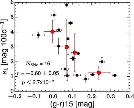
Anticorrelation between the slope of the plateau (s1) in the V band and the (g − r) colour at epoch 15 d. The results of Monte Carlo simulations on the statistics of these two variables are noted at the bottom of the figure, in a similar way to Fig. 4.
6.4 Do redder SNe II have stronger metal-line equivalent widths?
The comparisons between colours at different epochs and the equivalent widths of different absorption lines show that, in general, bluer SNe II tend to have smaller equivalent widths. In Fig. 11, one example is displayed using the (u − g) colour at 15 d and the Fe ii λ5169 equivalent width (EWFe6). Correlations at different epochs, using other colours and with different spectral lines, can be found in Fig. A5.
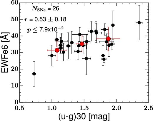
Correlation between the Fe ii λ5169 equivalent width (EWFe6) and the (u − g) colour at epoch 30 d. The results of Monte Carlo simulations on the statistics of these two variables are noted at the top of the figure in a similar way to Fig. 4.
The simplest explanation for these trends is that of an expected strong temperature dependence of both the observed colours and the strength of spectral lines. Again, these temperature differences could be related to differences in progenitor radii and/or the presence/absence of CSM interaction. However, when interpreting these results, one needs to be aware of the effect of line strengths on SN II magnitudes at specific bandpasses because of their presence within those bandpasses (see Fig. 6). If, for example, we only see these correlations using the (u − g) colour, it could be due a filter selection effect. If the Pearson factors are stronger with one colour than the others (u − g in this work), one could argue that is simply because a deeper absorption line (larger equivalent width) reduces the brightness in the filter containing the line — i.e. that the colour is caused by line blocking and not temperature effects. However, it is difficult to estimate this effect because a ‘true’ temperature is not easily extracted from our data. We note that the u band is strongly affected by line blanketing from millions of blended iron-group lines (mostly Ti iii and Fe ii; Kasen & Woosley 2009) that cannot be resolved.
Additionally, Dessart et al. (2014) show that a secondary effect affecting the colour is that caused by progenitor metallicity. Lower metallicity leads to smaller line strengths at a given temperature (colour). Since (u − g) shows stronger correlations with the equivalent widths of different elements than do other colours, we test to see if a relation exists between (u − g) and metallicity. As a metallicity proxy, we use the values from Anderson et al. (2016), which are derived using the N2 diagnostic (Marino et al. 2013, hereafter M13). We do not find statistical evidence of a such relationship. Nor do we detect a correlation between the metallicity and the slopes of the colour curves as theoretically suggested by Dessart et al. (2013), where the authors showed that SNe II with lower metallicity have faster colour evolution (due to the dependence of pre-SN radius on progenitor metallicity).
6.5 Do redder SNe II have faster ejecta velocities?
From our analysis, a correlation between the velocity at 50 d of different lines (H α, H β, Fe ii, ScFe, and ScM) and the (g − r) colour (to a lesser extent g − Y) at later epochs (50–70 d) is found. Redder SNe II have faster ejecta velocities. As an example, the correlation between the H α velocity and the colour (g − r) at 70 d is displayed in Fig. 12. Such a correlation has not been predicted (to our knowledge) by any explosion models, and its physical origin is unclear. However, as above, we note the possibility of a direct influence of the spectral-line properties on the measured colour: Fig. 12 correlates a colour using the r-band (which contains H α) with a measured property of H α.
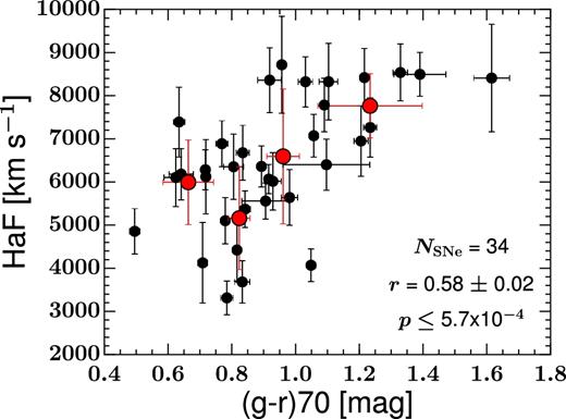
Correlation between the H α velocity (HaF) and the (g − r) colour at epoch 70 d. The results of Monte Carlo simulations on the statistics of these two variables are noted at the bottom of the figure in a similar way to Fig. 4.
6.6 Intrinsic colours
To support our hypothesis that the SN II colour diversity is driven by intrinsic differences, in this section we propose a ‘reductio ad absurdum’. If SN II colour diversity were dominated by host-galaxy extinction, then a sample of SNe II devoid of reddening should display roughly identical colours. To proceed, we follow the same steps as outlined in Section 5. First, for our low-reddening SN II sample, we select SNe II that are located away from host-galaxy nuclei and with no Na i D absorption, leading to a set of 19 SNe II.
Fig. 13 shows (B − V) colour curves for our full sample, along with the unreddened subsample composed of 19 SNe II displayed in distinct colours (blue). None of the unreddened colour curves is located on the top of the plot; they do not have the reddest colours. This is to be expected given that extinction makes objects redder, and that we grant that some SNe II within the sample probably suffer from significant extinction. However, the important observation is that this ‘unreddened’ sample spans a wide range in SN II colours, extending from (B − V) (at 50 d) of ∼0.70 mag (SN 2004fx) to (B − V) (at 50 d) of ∼1.13 mag (SN 2009N). Indeed, ∼75 per cent of the full sample falls within this range of colours, suggesting that (at least) this same percentage of SNe II suffers from negligible host-galaxy extinction. One can therefore conclude that significant dispersion exists in intrinsic SN II colours and that this dispersion dominates observed SN II colours.
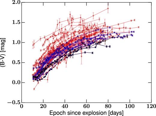
(B − V) curves for the entire sample (57 SNe II) are shown in red. Blue light curves represent our unreddened subsample (19 SNe II), while in black the bluest SNe from the unreddened subsample are shown (SN 2004fx, SN 2005dz, SN 2008M, and SN 2009bz).
With respect to colour evolution, for this subsample we derive a median value of 2.26 ± 0.51 mag 100 d−1, 0.74 ± 0.22 mag 100 d−1, and 37.9 ± 7.4 d for s1, (B − V), s2, (B − V), and Ttrans, (B − V), respectively. These values are consistent with the values derived for the whole sample (2.65 ± 0.62, 0.77 ± 0.26, and 37.7 ± 4.3 d, respectively) but also with the ‘reddened’ subsample (2.69 ± 0.66, 0.81 ± 0.26, and 37.6 ± 5.6 d, respectively). This suggests that SNe II display distinct colours and colour evolution independent of any host-galaxy extinction suffered by each event.
Finally, to conclude our tests, as suggested by Burns et al. (2014), Stritzinger et al. (2018), and Galbany et al. (2016, 2017) with respect to SNe II, we can restrict our unreddened subsample to only the bluest objects (SN 2004fx, SN 2005dz, SN 2008M, and SN 2009bz). Again, if the colour were caused only by dust extinction, these four SNe II with the bluest colours should have roughly identical colours. The colour-curve parameters for all the colours are displayed in Table 4; we note that the values obtained for this lowest-reddening subsample do not follow the same trend and also exhibit significant diversity. For example, SNe II with higher s1, (B − V) values display both smaller or larger s2, (B − V) values (SN 2005dz and SN 2009bz, respectively). The fact that even for this restricted subsample, the colour curves also show diversity, is consistent with our previous conclusions and suggests that intrinsic colour diversity is the origin of most of the observed differences.
Unreddened subsample colour-curve parameters.
| Parameters | SN 2004fx | SN 2005dz | SN 2008M | SN 2009bz | Mean |
|---|---|---|---|---|---|
| s1, (B − V) | 1.69 (0.24) | 2.22 (0.13) | 2.30 (0.15) | 2.17 (0.08) | 2.10 (0.24) |
| s2, (B − V) | 0.50 (0.14) | 0.26 (0.08) | 0.89 (0.17) | 0.95 (0.09) | 0.65 (0.28) |
| Ttrans, (B − V) | 36.8 (3.3) | 43.9 (1.7) | 45.4 (3.5) | 36.2 (1.5) | 40.6 (4.2) |
| s1, (u − g) | 6.51 (0.48) | 5.50 (0.36) | 6.38 (0.38) | 6.66 (0.26) | 6.26 (0.45) |
| s2, (u − g) | 1.63 (0.47) | ⋅⋅⋅ (⋅⋅⋅) | ⋅⋅⋅ (⋅⋅⋅) | 3.33 (0.93) | 2.48 (0.85) |
| Ttrans, (u − g) | 29.9 (2.1) | ⋅⋅⋅ (⋅⋅⋅) | ⋅⋅⋅ (⋅⋅⋅) | 32.5 (4.1) | 31.2 (1.3) |
| s1, (g − r) | 1.34 (0.10) | 1.72 (0.14) | 1.91 (0.08) | 1.72 (0.08) | 1.67 (0.21) |
| s2, (g − r) | 0.23 (0.07) | 0.06 (0.07) | 0.77 (0.05) | 0.54 (0.06) | 0.40 (0.26) |
| Ttrans, (g − r) | 33.9 (1.7) | 41.1 (2.0) | 39.3 (1.7) | 33.4 (1.3) | 36.9 (3.5) |
| s1, (g − Y) | ⋅⋅⋅ (⋅⋅⋅) | 2.35 (0.18) | 2.92 (0.17) | 2.92 (0.16) | 2.73 (0.27) |
| s2, (g − Y) | ⋅⋅⋅ (⋅⋅⋅) | 0.18 (0.13) | 0.84 (0.08) | 0.82 (0.19) | 0.61 (0.30) |
| Ttrans, (g − Y) | ⋅⋅⋅ (⋅⋅⋅) | 43.1 (1.0) | 39.9 (1.6) | 35.1 (2.0) | 39.4 (3.3) |
7 CONCLUSIONS
An extensive analysis of SN II colour curves using four different colours, together with their correlations with spectroscopic and photometric parameters, has been presented in this work. Here, we list our main conclusions:
SN II colour curves consist of two regimes that correlate: SNe II with steeper initial colour curves also have steeper colour curves during the plateau phase.
The colour evolution depends on the initial conditions. Bluer SNe II at 15 d after explosion are also bluer at 70 d after explosion.
SNe II form a continuous population in observed colours, consistent with other recent light-curve analyses finding an absence of a clear separation of these events into distinct classes.
Redder SNe II have fainter absolute magnitude at maximum. This correlation seems to originate from intrinsic colours, not from dust effects. Progenitor radius differences, together with the presence or absence of CSM close to progenitor stars, are the probable causes of this relation.
An intrinsic range in SN II colours of ∼0.70–1.13 mag in (B − V) is derived at 50 d post-explosion, with ∼75 per cent of the current sample falling within these limits. Such large intrinsic diversity is observed at all epochs.
Fast-declining SNe II (SNe IIL) are redder at later epochs (50d–70d); however, they appear bluer at early epochs (15–30 d).
At all epochs, redder SNe II have larger metal-line equivalent widths.
The strength of the H α absorption line (Haabs) anticorrelates with the slope of the colour curve during the plateau phase (s2, colour).
Redder SNe II at later epochs (50–70 d) seem to have faster ejecta velocities. However, the correlation is not seen in bluer filters.
The exact (intrinsic) physical origin of the observed colour differences and their correlation with other SN II transient properties in still not well understood. Contemporary work — especially at early epochs – suggests that SN II progenitors may not explode into a clean environment, but rather interact with CSM of various densities and extensions. When such interaction occurs, it is likely to complicate our understanding of SN II colours and observations in general, especially with respect to constraints on progenitor radius.
Additional early-time multicolour observations can aid our understanding and attempt to isolate the dominant progenitor properties producing observed diversity at different epochs. In addition, higher resolution spectra of SNe II (than those generally obtained by the SN community) would help to definitively tie down the degree of host-galaxy reddening affecting observed colours. Such observations and advances in our understanding will bring added confidence to our use of SNe II as distance indicators, allowing a better understanding of colour-term corrections. In this way, we will continue to better understand the progenitor systems of the most populous terminal stellar explosions, SNe II, while also refining their use as astrophysical probes.
ACKNOWLEDGEMENTS
We thank the referee for their thorough reading of the manuscript, which helped clarify and improve it. The work of the CSP-I has been supported by the NSF under grants AST–0306969, AST–0607438, and AST–1008343. Support for A.V.F.’s supernova research group at U.C. Berkeley has been provided by NSF grant AST–1211916, the TABASGO Foundation, Gary and Cynthia Bengier (T.d.J. is a Bengier Postdoctoral Fellow), the Christopher R. Redlich Fund, and the Miller Institute for Basic Research in Science (U.C. Berkeley). L.G. was supported in part by the NSF under grant AST–1311862. M.H. acknowledges support from the Ministry of Economy, Development, and Tourism's Millennium Science Initiative through grant IC120009, awarded to The Millennium Institute of Astrophysics (MAS). M.D.S. acknowledges funding by a research grant (13261) from the VILLUM FONDEN. E.Y.H. acknowledges support provided by NSF grant AST–1613472 and by the Florida Space Grant Consortium.
This research has made use of the NASA/IPAC Extragalactic Database (NED), which is operated by the Jet Propulsion Laboratory, California Institute of Technology, under contract with the National Aeronautics and Space Administration (NASA), and of data provided by the Central Bureau for Astronomical Telegrams. The work is also based on observations obtained at the Gemini Observatory, which is operated by the Association of Universities for Research in Astronomy, Inc., under a cooperative agreement with the NSF on behalf of the Gemini partnership: the NSF, the STFC (United Kingdom), the National Research Council (Canada), CONICYT (Chile), the Australian Research Council (Australia), CNPq (Brazil), and CONICET (Argentina). This research used observations from Gemini programs GN-2005A-Q-11, GN-2005B-Q-7, GN-2006A-Q-7, GS-2005A-Q-11, GS-2005B-Q-6, and GS-2008B-Q-56.
Footnotes
Throughout the rest of this text we refer to SNe II as the two historical groups, SNe IIP (plateau) and SNe IIL (linear), since recent studies indicate a relatively continuous distribution (Anderson et al. 2014; Sanders et al. 2015; Galbany et al. 2016; Valenti et al. 2016; see also Rubin et al. 2016).
To obtain the lower limit, we use the free p-value calculator provided by Dr. Daniel Soper: http://www.danielsoper.com/statcalc/calculator.aspx?id=44.
Fisher test or Wald test.
While here we generally argue that our results are not dominated by uncorrected host-galaxy extinction, there is still the possibility that some specific findings are driven by the effects of dust extinction.
REFERENCES
APPENDIX A
In the main body of this paper, we have shown an overview of our analysis and conclusions, without discussing all the correlations found in this SN II colour-curve study. For completeness, in this appendix several more figures are presented.
A1 Colour-curve fitting
In this section, additional examples of (B − V) colour fitting are shown in Fig. A1, together with examples of the (u − g), (g − r), and (g − Y) colour fitting. As explained is the main body of this paper, when the data are well sampled, we clearly see two regimes with two different slopes as noted by Patat et al. (1994), but in our case with a much larger set of objects.
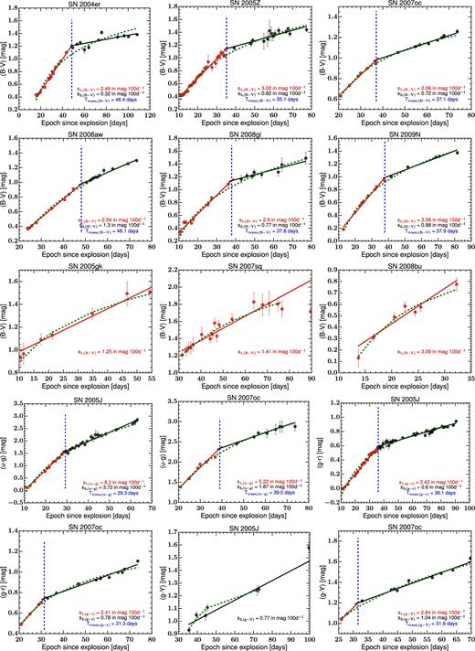
Example of the colour-curve parameters measured for each SN. The two slopes, s1, (X − Y) and s2, (X − Y), are represented in red and black, respectively (when two slopes are seen). The epoch of the transition if it exists, Ttrans, (X − Y) is shown in blue. The colours (B − V), (u − g), (g − r), and (g − Y) are represented. Power-law fitting is shown with the green dashed line.
A2 Colour-curve parameter correlation
In this section, more examples of the correlations between the two slopes seen in the colour curves are displayed in Fig. A2.
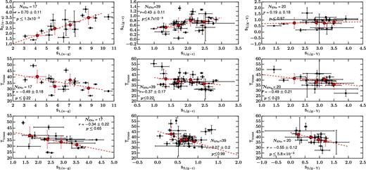
Correlations between measured parameters of the SN II colour curves: (u − g) (left), (g − r)(middle), and (g − Y) (right). In all of the panels, the same structure is displayed: top, s1, colour with s2, colour both expressed in mag (100 d)−1; middle, s1, colour with Ttrans, colour (in days); bottom, s2, colour with Ttrans, colour. In each panel, the number of SNe is listed, together with the Pearson factor and the p-value (p).
A3 Are redder SNe II less luminous?
In this section, all correlations between the colour and the absolute magnitude are shown. The relation between the absolute magnitude at maximum brightness and the colour is also presented for different combinations of colour, as shown in Fig. A3.
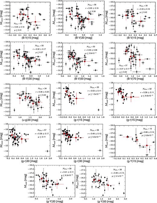
Correlation between the colour and the absolute magnitude at different epochs. The results of Monte Carlo simulations on the statistics of the variables are noted, similarly to Fig. 4.
A4 Are fast-declining SNe II redder?
In this section, all correlations between the colour and the slopes of the V-band light curve are presented. First, at the top of Fig. A4, the relation between s2 and the colour at later epochs is displayed. In the bottom of the figure, correlations between the colour at early times and s1 are displayed.
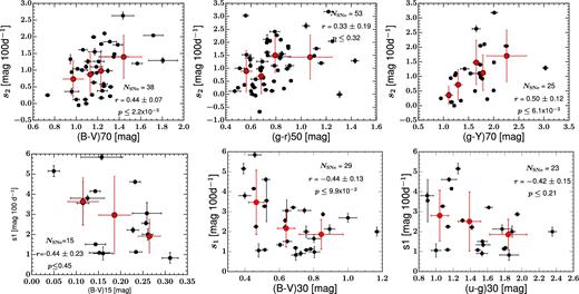
Correlation between the slopes of the V-band light curve (s1 and s2) and the colours. The results of Monte Carlo simulations on the statistics of these two variables are noted, similarly to Fig. 4.
A5 Are SNe II with smaller metal-line equivalent widths redder?
All correlations between the colour and the equivalent widths of lines of different elements are showed in Fig. A5.
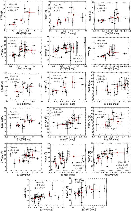
Correlation between the absorption-line equivalent widths and the colours. The results of Monte Carlo simulations on the statistics of these two variables are noted, similarly to Fig. 4.
A6 Correlation between Haabs and the colour slope
All correlations between the colour slope after transition and the strength of the H α absorption line are shown in Fig. A6.
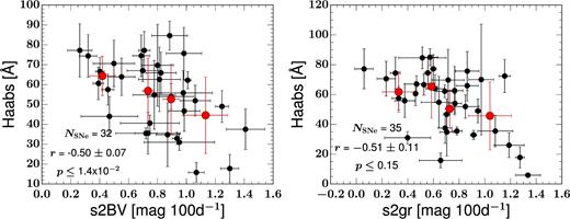
Inverse correlations between s2, (B − V) and the strength of the H α absorption line (Haabs), in the sense that SNe II with a fast cooling after transition show weaker H α absorption lines. The results of Monte Carlo simulations on the statistics of these two variables are noted at the bottom, similarly to Fig. 4.
A7 Are SNe II with faster ejecta velocities redder?
All correlations between the colour and the velocities of different elements are showed in Fig. A7. We also display a trend between the colour (g − Y) at epoch 15 d and the velocities of HaF and ScM. For these correlations, we have only 8 and 6 objects, respectively.
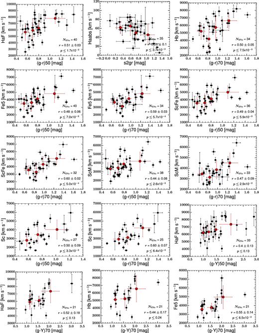
Correlation between the ejecta velocities and the colours. The results of Monte Carlo simulations on the statistics of these two variables are noted, similarly to Fig. 4.
APPENDIX B:
In this appendix, the colour evolution for the entire sample and the three other colours used in this work are displayed in Fig. B1.
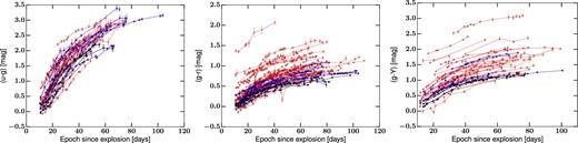
Colour curves for the whole sample are shown in red (57 SNe II). Blue light curves represent our unreddened subsample (19 SNe II), while in black the bluest SNe II from the unreddened subsample are shown (SN 2004fx, SN 2005dz, SN 2008M, and SN 2009bz). The colours (u − g), (g − r), and (g − Y) are displayed in the left, middle, and right panels, respectively.
