


Abstract
At least |$25\,\,\rm{per\,\,cent}$| of white dwarfs show atmospheric pollution by metals, sometimes accompanied by detectable circumstellar dust/gas discs or (in the case of WD 1145+017) transiting disintegrating asteroids. Delivery of planetesimals to the white dwarf by orbiting planets is a leading candidate to explain these phenomena. Here, we study systems of planets and planetesimals undergoing planet–planet scattering triggered by the star's post-main-sequence mass loss, and test whether this can maintain high rates of delivery over the several Gyr that they are observed. We find that low-mass planets (Earth to Neptune mass) are efficient deliverers of material and can maintain the delivery for Gyr. Unstable low-mass planetary systems reproduce the observed delayed onset of significant accretion, as well as the slow decay in accretion rates at late times. Higher-mass planets are less efficient, and the delivery only lasts a relatively brief time before the planetesimal populations are cleared. The orbital inclinations of bodies as they cross the white dwarf's Roche limit are roughly isotropic, implying that significant collisional interactions of asteroids, debris streams and discs can be expected. If planet–planet scattering is indeed responsible for the pollution of white dwarfs, many such objects, and their main-sequence progenitors, can be expected to host (currently undetectable) super-Earth planets on orbits of several au and beyond.
1 INTRODUCTION
A significant fraction of white dwarfs (WDs) show evidence of possessing remnant planetary systems. This evidence comes in the form of photospheric metal pollution (e.g. Zuckerman et al. 2003; Koester, Gänsicke & Farihi 2014), circumstellar discs of dust and gas (e.g. Zuckerman & Becklin 1987; Graham et al. 1990; Gänsicke et al. 2006; Farihi 2016), and in the case of WD 1145+017, a photometric light curve interpreted as eclipses of the WD by disintegrating asteroids (Vanderburg et al. 2015; Gänsicke et al. 2016; Rappaport et al. 2016; Hallakoun et al. 2017). Metal-polluted WDs are of particular interest for exoplanet science, as they yield insight into the elemental compositions of extrasolar planets and asteroids: The gravitational settling time-scales in most WD atmospheres are astronomically short, and so any pollution reflects the composition of recently-accreted material (Zuckerman et al. 2007; Koester 2009). In this way, the composition of bodies accreted on to WDs has been compared to Solar system objects, such as chondritic meteorites and the bulk Earth (e.g. Gänsicke et al. 2012; Jura & Young 2014; Xu et al. 2014; Zuckerman & Young 2017), and in rare cases Kuiper Belt Objects (Xu et al. 2017).
The prevailing paradigm attributes such photospheric pollution to the accretion of objects originating from orbits of at least several au in the planetary system. Prior to becoming a WD, the star's asymptotic giant branch (AGB) radius reaches values of roughly 1–5 au for stars of mass 1–5M⊙, resulting in the engulfment of planets with comparable perihelion distances; the boundary between survival and engulfment is determined by the opposing effects of orbital decay due to tidal deformation of the star, and orbital expansion due to stellar mass-loss (e.g. Villaver & Livio 2009; Mustill & Villaver 2012; Villaver et al. 2014). Bodies engulfed by the star are expected to be destroyed unless they are at least of several Jovian masses (Villaver & Livio 2007; Nordhaus et al. 2010; Staff et al. 2016). Furthermore, the pollutant bodies themselves cannot have very small periapsis distances when the star is a giant, lest they be engulfed and destroyed before the star becomes a WD. Taken together, these statements imply the presence of not only a reservoir of pollutant bodies, but also one or more objects capable of gravitationally perturbing these pollutants on to collision trajectories with the WD, all on orbits of several au or beyond. These trajectories take the bodies either on to a direct collision course with the WD or, more likely, cause their tidal disruption once the body crosses the Roche limit at around a Solar radius (e.g. Debes, Walsh & Stark 2012; Veras et al. 2014). This disruption is then followed by the formation of a circumstellar disc, as fragments are subjected to collisional or radiative forces (Jura 2008; Veras et al. 2015; Brown, Veras & Gänsicke 2017).
Thus, the general narrative is that the outer regions of planetary systems survive the AGB, and can then feed material on to the WD by dynamical evolution over the WD's lifetime. The importance of these ‘outer regions’ (beyond a few au), and the relatively large mass of the progenitor stars (∼2 M⊙), presents a challenge to modellers, because this is a parameter space inaccessible to most planet-hunting surveys. However, they also present an opportunity, because by identifying system architectures that do or do not lead to the observed incidence and rates of planetesimal accretion on to WDs, we can constrain the architectures of planetary systems in this otherwise inaccessible parameter space.
Changes to the star as it evolves have significant consequences for orbiting bodies. Notably, stellar mass loss towards the end of the AGB changes the planets’ dynamics and stability. The increase in the planet:star mass ratios following AGB mass loss makes planet–planet interactions stronger and can even destabilize previously stable systems. Although the outer planets of the Solar system are sufficiently widely spaced that they will remain stable when the Sun is a WD (Duncan & Lissauer 1998; Veras 2016b), Debes & Sigurdsson (2002) noted that this will not be the case for more tightly packed systems, hypothesising that planetary systems, destabilized by mass loss, may be responsible for the observed pollution in WDs.
In recent years, several studies have extended and complemented the work of Debes & Sigurdsson (2002), who focused on the stability of systems experiencing a toy model of stellar mass loss. Exploiting faster computers, Veras et al. (2013a) and Mustill, Veras & Villaver (2014) were able to integrate two- and three-planet systems, respectively, over 5 Gyr with stellar mass and radius evolution taken from pre-computed stellar models. Veras et al. (2016) extended these studies to planets of unequal masses and of lower masses. An alternative line of attack was initiated by Bonsor, Mustill & Wyatt (2011), who studied the destabilization of particles orbiting close to a single planet on a circular orbit. Subsequent work showed that this requires a carefully constructed chain of planets to feed the material all the way to the central object (Bonsor, Augereau & Thébault 2012), but Frewen & Hansen (2014) showed that a low-mass, eccentric planet embedded in a planetesimal disc can efficiently feed material to the star; Antoniadou & Veras (2016) showed that a planet on a circular orbit cannot. Debes et al. (2012) studied the broadening of Kirkwood gaps in Asteroid Belt analogues, finding that typical belt masses had to be several hundred times greater than our own Asteroid Belt to provide the observed accretion rates. Recently, Payne et al. (2016, 2017) have investigated moons liberated from their planets during planet–planet scattering as a source of pollution. Although most papers (including this present one) focus on the planetary systems of single stars, a number have studied the effects of perturbations from binary companions (Bonsor & Veras 2015; Hamers & Portegies Zwart 2016; Petrovich & Muñoz 2017; Stephan, Naoz & Zuckerman 2017) as potential drivers of WD pollution. The rich dynamics of post-main-sequence (MS) planetary systems were recently reviewed by Veras (2016a).
The origin of the planetesimals accreted on to the WD can be constrained by a spectroscopic determination of the composition of the pollutant material. This methodology is fully equivalent to the analysis of meteorites accreted on to the Earth, from which fundamental information about the composition of the Solar system is inferred. Detailed abundance studies of multiple elements for ∼20 debris-polluted WDs (Zuckerman et al. 2007; Klein et al. 2010; Gänsicke et al. 2012; Jura & Young 2014; Xu et al. 2014; Farihi et al. 2016) and ∼300 additional systems in which a handful of elements were detected (Jura & Xu 2013; Hollands et al. 2017) demonstrate that the disrupted exo-planetesimals show a wide range of bulk compositions, but overall resemble rocky bodies within the inner Solar system, with one exception being the Kuiper-belt analogue of Xu et al. (2017). In addition, a small number of systems have been found to actively accrete water-rich planetesimals (Farihi, Gänsicke & Koester 2013; Raddi et al. 2015), and there is further evidence of a larger population of water-bearing planetary bodies orbiting WDs (Gentile Fusillo et al. 2017), which highlights the general potential of water delivery to dry inner planets. On the whole, however, the accreted material resembles asteroids, constraining either the place of origin of the accreted planetesimals or their evolution under the large luminosities of red giant branch (RGB) and AGB stars.
In this paper, we explain WD accretion rates by evaluating the efficiency of planet–planet scattering in the presence of planetesimal discs, synthesizing and building on a number of previous works. The key ingredients are as follows:
The finding by Frewen & Hansen (2014) that low-mass eccentric planets can efficiently feed material to a WD over long time-scales. This paper did not, however, explain how the required configuration of a single low-mass planet with a high eccentricity (e ∼ 0.6), embedded in a disc of low-eccentricity planetesimals, could attain its initial configuration.
The result from Veras & Gänsicke (2015) and Veras et al. (2016) that instabilities in systems of wide-orbit, low-mass planets orbiting WDs can take Gyr to resolve, during which time planets ‘meander’, spending significant periods of time on eccentric orbits before ejection occurs. We posit that these instabilities offer a natural way for the eccentric planets studied by Frewen & Hansen (2014) to attain the required configuration.
The observation from both transit surveys (Fressin et al. 2013) and radial-velocity surveys (Cumming et al. 2008; Mayor et al. 2011) that lower mass planets are more common than giant planets, with several 10s per cent of stars hosting at least one super-Earth or Neptune within ∼0.5 au. Microlensing reveals a comparable occurrence rate of planets on few au orbits, albeit around lower-mass stars (Shvartzvald et al. 2016). Although extrapolation can be dangerous, it is reasonable to speculate that many low-mass planets exist on orbits of a few au and beyond.
The use of a modified MercuryN-body integrator, which allows us to follow accurately the evolution of planetary systems, including test particles for several Gyr. Our integrator is based on that described by Veras et al. (2013a, where we adapted the Bulirsch–Stoer integrator), but has been modified to make use of the more accurate RADAU algorithm: In Mustill et al. (in preparation), we show that this accurate integrator is essential to accurately determine instability time-scales for the systems we consider.
We first conduct simulations of unequal-mass three-planet systems over host stars’ MS and WD lifetimes (for 5 Gyr), to explore the range of stability times for planetary systems of different masses (Section 2). We then run a smaller number of integrations of three-planet systems incorporating discs of test particles, to study the delivery rate of these bodies to the WD (Section 3). We study both ‘inner belts’ of asteroidal bodies interior to the planets’ orbits, and ‘outer belts’ of cometary bodies exterior to the planets’ orbits, to compare the relative efficiencies of delivery of the two populations. A cartoon showing the system configurations we study is shown in Fig. 1. We then discuss these results in the context of the latest observations of WD pollution (Section 4), and conclude in Section 5.
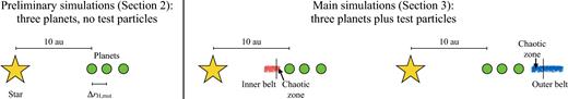
Schematic set-up for our simulations. In Section 2, we consider three-planet systems orbiting a star of initial mass 3 M⊙. In Section 3, we include test particles in either an inner belt or an outer belt, in each case extending from within the nearest planets chaotic zone to more distant stable orbits.
2 PRELIMINARY INTEGRATIONS: NO TEST PARTICLES
2.1 Setup
We run several sets of integrations of three-planet systems with no test particles in order to identify architectures of interest for more detailed study. These integrations themselves extend the range of system architectures covered in previous studies: where Debes & Sigurdsson (2002) and Mustill et al. (2014) both studied equal-mass systems, Veras et al. (2016) studied unequal-mass systems based on permutations of the Solar system planets. Here, we extend the variety of unequal-mass systems, considering three mass-ranges: roughly Saturn to super-Jupiter (S2SJ), Neptune to Saturn (N2S), and super-Earth to Neptune (SE2N).
We take a 3 M⊙ star for all our simulations. This is at the upper range of the progenitor masses of polluted WDs (Koester et al. 2014), but allows our simulations to be conducted in a reasonable time (recall the very strong dependence of stellar MS lifetime on initial mass: A 3 M⊙ star will live for ∼0.5 Gyr but a 1 M⊙ star for ∼12 Gyr). The star is evolved with SSE (Hurley, Pols & Tout 2000), and the output file containing mass and radius is fed to the modified Mercury integrator (Veras et al. 2013a, Mustill et al, in preparation; and see Appendix A). The star becomes a WD of mass 0.75 M⊙ at 477.6 Myr, after attaining a peak AGB radius of 2.85 au. Stellar mass loss is implemented in Mercury by adjusting the stellar mass both at major integrator time-steps and at all sub-intervals of these time-steps (Veras et al. 2013a). Mass loss is assumed to be isotropic (a good approximation for bodies at the orbital radii we consider, Veras, Hadjidemetriou & Tout 2013b), but we naturally capture any non-adiabatic effects from rapid mass loss. 1 Systems are integrated for 5 Gyr with the RADAU integrator from the Mercury package (Chambers 1999), with a tolerance parameter of 10−11. Particles are removed from the simulation when they are ejected, or collide with a planet or with the physical radius of the star. We record the pericentres of bodies throughout the integrations, allowing us to post-process the simulation data to check for the intrusion of particles past the Roche limit of the WD at ∼0.005 au.
As in our previous works, we set the inner of the three planet's initial semi-major axis to 10 au. This allows faster integrations (thanks to the larger timestep for a given tolerance), but also ensures that the planets we consider are well beyond the reach of tidal forces when the star is a large AGB object2 (Mustill & Villaver 2012; Nordhaus & Spiegel 2013). The limit for surviving tidal inspiral is ∼4 au for a Jovian planet on a circular orbit around a 3 M⊙ primary, and ∼2.5 au for Earth-mass planets. Planets on slightly wider orbits will still experience some tidal orbital decay even though they avoid engulfment. Although 10 au is conservative for planets on circular orbits, it also ensures that our inner belts of test particles in the full integrations described in the next section are also safe from engulfment on the AGB.
2.1.1 Generating a planet population
Unfortunately, the properties of planet populations (most importantly for our purposes, mass and semimajor axis) are almost entirely unknown around both WDs and their largely intermediate-mass progenitors. Direct imaging is sensitive to very massive super-Jupiter planets from 10s to 100s of au, but with the exception of the extremely wide-orbit (∼2500 au) companion to WD 0806-661 (Luhman, Burgasser & Bochanski 2011) there have been no detections of planetary companions to single WDs (Debes, Sigurdsson & Woodgate 2005a,b; Burleigh et al. 2008; Zinnecker & Kitsionas 2008; Hogan, Burleigh & Clarke 2009; Xu et al. 2015). Searches for IR excess are sensitive to closer, unresolved, companions, but have similarly given negative results (Farihi, Becklin & Zuckerman 2008). Timing of stellar pulsations, sensitive to giant planets at a few au, has also given no robust detections (Mullally et al. 2008; Winget et al. 2015). Finally, there have been no detections of transiting planets (as opposed to asteroids) orbiting WDs on small orbits ≲ 0.1 au (Faedi et al. 2011; Fulton et al. 2014; Sandhaus et al. 2016; van Sluijs & Van Eylen 2017). Currently, the strongest limits come from Pan-STARRS1 for giant planets (|${\lesssim }0.1\,\,\rm{per\,\,cent}$| for Jovian planets at 0.01 au; Fulton et al. 2014) and from K2 for smaller planets (|${\lesssim }25\,\,\rm{per\,\,cent}$| for Earth-radius planets at 0.01 au; van Sluijs & Van Eylen 2017), although occurrence rates beyond 0.05 au are weak to non-existent.
The progenitors of WDs may be probed for planets with radial velocity surveys when they have evolved to leave the MS. Reffert et al. (2015) found that the occurrence rate of Jovian planets peaks for stellar masses around 2 M⊙, at |$5\hbox{--}15\,\,\rm{per\,\,cent}$| (depending on whether one counts only the secure detections or includes candidates) on periods of up to a few years. Direct imaging surveys have probed orbits of several 10s of au for super-Jovian planets but, despite spectacular finds such as the four planets of HR 8799 orbiting a 1.5 M⊙ primary (Marois et al. 2008, 2010), the occurrence rate of such systems is low (|${\lesssim }10\,\,\rm{per\,\,cent}$|, Nielsen et al. 2013; Chauvin et al. 2015). Unfortunately, less massive planets remain undetectable, unless the object Fomalhaut b (Kalas et al. 2008) is, in fact, a super-Earth or ice giant surrounded by a dust cloud (Kennedy & Wyatt 2011).
This ignorance means that we must use a set of artificially constructed systems that cover a range of possible architectures for the outer regions of planetary systems orbiting intermediate-mass stars. We can however be guided by the much better understood populations of planets on smaller (≲1 au) orbits around Solar-type and M dwarf stars. Radial-velocity surveys have found that, within an orbital period of 100 d, around |$50\,\,\rm{per\,\,cent}$| of FGK stars have at least one detectable planet of mass msin i < 30 M⊕, whereas |${\sim }10\,\,\rm{per\,\,cent}$| host a gas giant msin i > 50 M⊕ with a period of up to 10 yr (Mayor et al. 2011). These numbers are in agreement with the statistics of transiting planet candidates from the Kepler mission, which found that |$50\,\,\rm{per\,\,cent}$| of stars have a planet of radius 0.8–22 R⊕ with a period less than 85 d and |$5\,\,\rm{per\,\,cent}$| host a giant planet (radius >6 R⊕) with a period less than 400 d (Fressin et al. 2013). Thus, low-mass planets are common close to the star. It is not unreasonable to speculate that low-mass (super-Earth or Neptune-like) planets may be equally common on wide orbits around the progenitors of WDs, although this depends on the properties of protoplanetary discs, and the pathways planet formation takes around these more massive stars.
A final consideration is the spacing of orbits in multiplanet systems. The eccentricity distribution of giant planets is explained if the majority of them (|${\sim }80\,\,\rm{per\,\,cent}$|, Jurić & Tremaine 2008; Raymond et al. 2011) were sufficiently tightly packed after formation that they experienced scattering early in their MS evolution. Systems slightly more widely spaced are prime candidates for destabilization following post-MS mass loss, whereas systems that have already experienced one instability on the MS often experience a second after the star becomes a WD (Mustill et al. 2014). The time-scale for a system to experience instability can be crudely estimated from the planets’ separations in mutual Hill radii (Chambers, Wetherill & Boss 1996). For observed Kepler systems of four or more planets, Pu & Wu (2015) found that the distribution of separations peaks at 14 mutual Hill radii. Lissauer et al. (2011) and Fabrycky et al. (2014) estimated, from the empirical scalings of Smith & Lissauer (2009), that a separation of nine mutual Hill radii should be the approximate limit for systems to remain stable to the mid-MS age of a typical star, but nevertheless found a number of more tightly packed systems. Considering all Kepler multiples, Weiss et al. (2017) recently found that the median separation is ∼20 mutual Hill radii. If wider-orbit planets follow similar spacings, not all are expected to be destabilized by mass loss: Mustill et al. (2014) estimate the maximum limit for systems of three Earth-mass planets to be destabilized around WDs at around 18 single-planet Hill radii, or 14 mutual Hill radii.
Based on the above considerations, we construct the following simulation sets, each of 128 runs for a total of 1 536 runs:
s2sj-XYrh: Three giant planets, masses chosen from 100 to 1000 M⊕ (‘Saturn to super-Jupiter’). The innermost planet is placed at 10 au, and the subsequent planets are separated by x to y mutual Hill radii, where y = x + 2 and x ∈ {4, 5, 6, 7, 8}.
n2s-57rh: Three intermediate-mass planets, masses chosen from 10 to 100 M⊕ (‘Neptune to Saturn’). We perform a single set of runs in this mass range, with the inner planet again at 10 au and subsequent planets spaced by 5–7 mutual Hill radii.
se2n-XYrh: Three low-mass planets, masses chosen from 1 to 30 M⊕ (‘Super-Earth to Neptune’), with the inner planet at 10 au and subsequent planets separated by x to y mutual Hill radii, where y = x + 2 and x ∈ {5, 6, 7, 8, 9, 10}.
Extrapolating from the statistics of close-in planets discussed above, we expect the se2n runs to represent the mass range of perhaps the majority of the progenitor systems’ planets. However, our systems are rather tightly spaced compared to the average Kepler multiple.
For each planetary system, the masses of the planets are drawn independently from a distribution uniform in the logarithm of the mass, within the specified range. The initial eccentricities are zero, and inclinations are drawn in the range [0°, 1°] from a reference plane, with randomized longitudes of ascending node and mean anomalies. The left-hand panel of Fig. 1 illustrates the set-up.
2.2 Results
These preliminary integrations show the usual destabilizing effect of stellar mass loss on orbiting planets. Stellar mass loss triggers instability by increasing the planet:star mass ratio, increasing the size of the Hill spheres and broadening orbital resonances. An example is shown in Fig. 2. This system experiences one early instability on the MS (at around 2 Myr) before settling into a stable two-planet configuration. This configuration is itself destabilized following mass loss on the AGB, losing a second planet at around 0.9 Gyr, following several hundred Myr of planet–planet scattering.
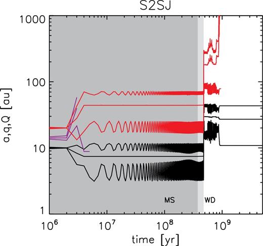
Example evolution of one system of three planets orbiting an evolving star, from simulation set s2sj-57rh. For each planet (shown in a different colour), the semi-major axis a, pericentre q, and apocentre Q are shown as a function of time. The stellar evolutionary state is shown as the background shading (dark for MS, light for end MS to end AGB, and white for WD). The system experiences an early instability, resulting in the ejection of one planet after a few Myr. The resulting two-planet configuration remains stable throughout the star's remaining MS lifetime, before mass loss just before 500 Myr results in a second instability and eventual ejection of another planet. Planet–planet scattering continues for several hundred Myr before eventual ejection.
Planetary instability may occur before or after AGB mass loss, or not at all, the time-scale being crudely set by the planetary separation (e.g. Chambers et al. 1996). We show the stages of evolution at which systems first lost planets, to collision or ejection, as a function of the initial separation in mutual Hill radii, in Fig. 3. As the separation increases, there is a trend away from instability before mass loss, to instability following mass loss, and finally to stability for the whole integration. This transition is not abrupt and considerable overlap exists between these regimes, as expected from previous studies (e.g. Chambers et al. 1996; Mustill et al. 2014). The transition is less abrupt for the lower mass planets. Instability may also be measured by the onset of orbit-crossing, and by this criterion, the instabilities at different ages are tabulated in Table 1. Again, we see a trend away from most instability occurring before AGB mass loss, to most instability occurring after AGB mass loss, to finally most systems being stable for the entire 5 Gyr integration time.
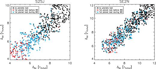
Integration outcomes for systems of three planets, as a function of the initial separation in mutual Hill radii between the inner two planets (Δbc) and the outer two planets (Δcd). Left-hand panel: s2sj runs (planet masses ‘Saturn to super-Jupiter’). Right-hand panel: se2n runs (planet masses ‘super-Earth to Neptune’). As the separation is increased, there is a transition from systems unstable on the MS, to those destabilized by mass loss, to those stable throughout the integration, but the transition is not abrupt. We do not show here the n2s runs as we only considered a small range in separations, but the same trend is present.
Instabilities in triple-planet systems without test particles. “Instability” here refers to the onset of orbit-crossing or the loss (collision or ejection) of the first planet, if orbit-crossing is not picked up because of the discrete output intervals.
| # runs | # orbit crossing begins | # orbit crossing begins | |
|---|---|---|---|
| Simulation set | before WD forms | after WD forms | |
| S2SJ-46rh | 128 | 72 | 55 |
| S2SJ-57rh | 128 | 21 | 85 |
| S2SJ-68rh | 128 | 3 | 48 |
| S2SJ-79rh | 128 | 1 | 17 |
| S2SJ-810rh | 128 | 0 | 5 |
| N2S-57rh | 128 | 62 | 63 |
| SE2N-57rh | 128 | 99 | 29 |
| SE2N-68rh | 128 | 49 | 72 |
| SE2N-79rh | 128 | 17 | 91 |
| SE2N-810rh | 128 | 7 | 67 |
| SE2N-911rh | 128 | 3 | 42 |
| SE2N-1012rh | 128 | 0 | 17 |
We now consider the distribution of stellar ages at which instability occurs. Fig. 4 shows this distribution in different simulation sets. Each panel shows two kernel density estimates:3 One for the distribution of times at which orbit-crossing begins and one for the distribution of times at which planets are lost, be that due to ejection or collision with each other or with the star. The upper panels show the simulations with planets in the three mass ranges and initially spaced at 5–7 mutual Hill radii, some of the tightest spacings we considered. These simulation sets show spikes in the rate of the onset of orbit-crossing at very early times on the MS and again following AGB mass loss. In the s2sj set of massive planets, the times at which planets are lost closely track the times of onset of orbit-crossing: In these systems, the instabilities quickly result in the loss of one or more planets, usually to ejection. In contrast, in the lower-mass simulation sets, the times at which planets are lost follow a much flatter distribution, with no sudden spike following AGB mass loss for the lowest mass planets (se2n). Instabilities in these systems can take many Gyr to resolve, and many unstable systems in which the orbits have begun crossing actually retain all three planets for the whole integration. The lower panels show the same distributions, but summed over all initial separations for the s2sj and se2n mass ranges. The time-scale to begin orbit-crossing is a strong function of separation, and so the incorporation of more widely spaced systems broadens the tail of systems that experience late instabilities. Most instabilities, however, still begin at young WD cooling ages of a few 100 Myr. The distribution of times at which planets are lost in the low-mass se2n systems remains rather flat; we shall see that this enables delivery of material to the WD for several Gyr in these systems.
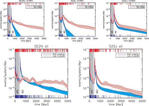
Kernel density estimates (and 1σ bootstrap confidence intervals) showing times at which instability occurs (here defined as the onset of orbit-crossing) and planets are lost (to collision or ejection) in preliminary integration sets (with no test particles). Top row: All runs in sets with planet spacings from 5 to 7 mutual Hill radii. Top left-hand panel: super-Earth to Neptune-mass planets, set se2n-57rh. Top centre: Neptune to Saturn-mass planets, set n2s-57rh. Top right-hand panel: Saturn- to super-Jupiter mass planets, set s2sj. Bottom row: All sets (all separations) for super-Earth to Neptune-mass planets (Bottom left-hand panel) and Saturn- to super-Jupiter mass planets (Bottom right-hand panel). Kernel density estimates are constructed with an adaptive-width (k-nearest neighbour) Gaussian kernel. Individual times of events are shown as ticks on the upper and lower axes. Background shading shows the star's evolutionary state, as in Fig. 2. In all panels, instabilities occur at a decreasing rate along the MS. Instabilities then spike following mass loss, after which the rate decays again. With higher mass planets (s2sj), the rate at which planets are lost closely tracks the rate at which orbit-crossing commences, but lower-mass planets show a more constant rate of planets being lost as it can take many Gyr to change the orbits sufficiently to eject a planet or force it to collide with the star.
The orbital expansion of the planets during the AGB closely followed the expectation for the adiabatic regime that eccentricity should not be excited. We did, however, find a moderate eccentricity excitation of a few per mil. Single planets placed at 10 and 20 au from our stars had their eccentricities excited to 0.0014 and 0.0034, respectively. Planets at larger separations will experience more eccentricity excitation. This can, for example, repopulate unstable chaotic regions surrounding a planet's orbit (Caiazzo & Heyl 2017). Pu & Wu (2015) found that, in terms of stability lifetime, increasing planetary eccentricity by ∼0.01 is roughly equivalent to reducing the separation by one mutual Hill radius. Planets on wider orbits than we have considered – a few 10s of au – will therefore experience destabilization slightly more often.
Having conducted the simulations without test particles described in this Section, we select three individual runs for further study. We take one from each of s2sj-57rh, n2s-57rh, and se2n-57rh and add in test particles, as described in the following Section. In each of these simulations, the planets were stable throughout the MS but unstable after AGB mass loss, providing an ideal scenario for WD pollution. Parameters for our selected runs are given in Table 2 .
Planetary parameters (masses, radii, and separation in mutual Hill radii) for the runs used in Section 3 for the full integrations including test particles.
| Run | Planet mass (M⊕) | Semimajor axis (au) | Separation (rH, mut) |
|---|---|---|---|
| s2sj | 276.9 | 10.00 | – |
| 462.3 | 14.58 | 5.95 | |
| 121.8 | 20.14 | 5.52 | |
| n2s | 98.3 | 10.00 | – |
| 65.2 | 12.63 | 6.12 | |
| 19.5 | 15.39 | 6.46 | |
| se2n | 1.3 | 10.00 | – |
| 30.6 | 11.60 | 6.74 | |
| 7.8 | 13.07 | 5.11 |
3 MAIN INTEGRATIONS: TEST PARTICLES INCLUDED
We now proceed to study the efficiency and rate of delivery of planetesimals to the WD by adding massless test particles to our simulations. The use of massless particles allows us to scale the simulation results to any belt mass, but requires that there be no significant gravitational effect of the planetesimals on the planets; most significantly, that there be no eccentricity damping. We show in the Appendix B that this is satisfied if each planet is ≳10 times more massive than the total planetesimal mass. For our lowest mass planets, this imposes a maximum belt mass of ∼0.1 M⊕.
The test particles in our simulations feel the gravitational force from the star and planets but do not experience non-gravitational forces. These can include gas drag from the stellar wind and stellar radiation forces, such as Poynting–Robertson drag and the Yarkovsky effect, which can all be significant when the star approaches the AGB tip (Bonsor & Wyatt 2010; Dong et al. 2010; Veras 2016a). These forces are size-dependent and their inclusion would require specifying a size distribution for the planetesimals, in addition to the added computational cost. We plan to investigate the effects of non-gravitational forces in future work.
We take each of our chosen integrations and clone it 20 times, retaining the same input positions and velocities for the planets. We then add 200 test particles to each integration: 10 integrations with all of the test particles interior to the innermost planet (runs *-inner) and 10 with all of them exterior to the outermost planet (runs *-outer). We also run one simulation in which the test particles are distributed between the orbits of the innermost and the outermost planet (run se2n-straddle). In total, we thus have 61 simulations and 12 200 test particles. Simulations are again run for 5 Gyr. Note that, as we use the adaptive-time-step RADAU algorithm, the evolution of the massive planets is not the same in each integration. In Mustill et al. (in preparation), we describe the tests that we conducted in order to verify that use of the RADAU integrator provides statistically robust results, even though each system's evolution is chaotic and affected by the integrator time-step (set by the orbits of the test particles and the close encounter history).
We set the limits of the planetesimal belts to slightly intrude into the chaotic zone of the innermost or outermost planet (Wisdom 1980). This allows for a natural sculpting of the belt over the star's MS lifetime, as well as for the natural expansion of the chaotic zone following AGB mass loss but before planetary instability (Bonsor et al. 2011; Frewen & Hansen 2014). Particles are distributed uniformly in semi-major axis within these belts. Limits on the initial belt semi-major axes are given in Table 3. The two right-hand panels of Fig. 1 illustrate the set-up, and an example initial configuration in a − e space can be seen in the top left-hand panel of Fig. 5.
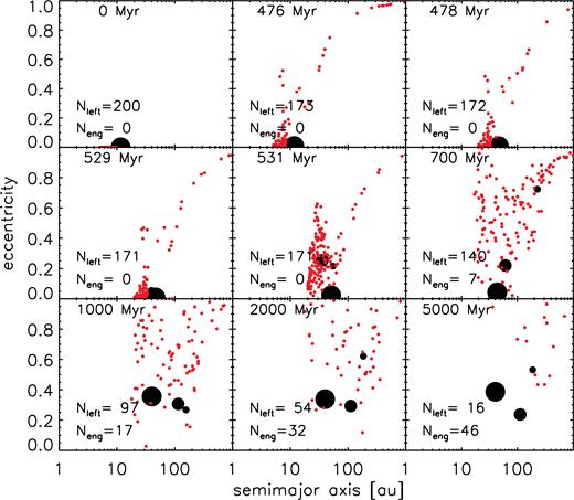
Time evolution of the run se2n-inner-07 with three low-mass planets (black, radius proportional to cube root of mass) plus an inner belt of 200 test particles (red). Each panel shows a different time snapshot; the cumulative number of particles to have been engulfed into the WD's atmosphere (Neng) and the number of particles remaining (Nleft) are shown at the bottom of each panel. Top left-hand panel: Initial state. Top centre: State just before significant mass loss at the AGB tip. Some belt particles have been scattered or ejected. Top right-hand panel: State after AGB mass loss. The entire system has expanded almost adiabatically. Middle and bottom rows: Development of the planetary instability and subsequent clearing of the belt. Orbit-crossing begins at around 530 Myr but all planets remain bound until the end of the integration at 5 Gyr. During this time 46 test particles (out of 173 surviving to the WD phase) collide with the WD, as their eccentricity is excited to near unity while their semi-major axes remain at a few tens of au.
Fates of the test particles in our simulation sets. We give the number of runs for each configuration (Nruns); the initial number of particles summed across those runs (Nparticles); the inner and outer edges of the planetesimal belt (ain and aout); the number of particles surviving when the star becomes a WD (Nsurv); the number colliding with the WD (Nengulf) and the fraction of the surviving particles that these represent (fengulf); and the number entering the Roche limit of the WD (NRoche) and the fraction of surviving particles that these represent (fRoche). 1In two of the ten S2SJ-wide-outer runs the planets were stable and we ignore them when compiling these statistics. No particles struck the WD in these runs.
| Simulation set | Nruns | Nparticles | ain [au] | aout [au] | Nsurv, WD | Nsurv, 5Gyr | Nengulf | fengulf | NRoche | fRoche |
|---|---|---|---|---|---|---|---|---|---|---|
| S2SJ-outer | 81 | 1600 | 25.0 | 45.0 | 1517 | 27 | 11 | 0.7 per cent | 72 | 4.7 per cent |
| S2SJ-inner | 10 | 2000 | 5.0 | 8.5 | 1069 | 6 | 25 | 2.3 per cent | 142 | 13.3 per cent |
| N2S-outer | 10 | 2000 | 16.5 | 25.0 | 1576 | 95 | 85 | 5.4 per cent | 342 | 21.7 per cent |
| N2S-inner | 10 | 2000 | 5.0 | 9.0 | 1568 | 64 | 190 | 12.1 per cent | 585 | 37.3 per cent |
| SE2N-outer | 10 | 2000 | 13.5 | 25.0 | 1785 | 184 | 138 | 7.7 per cent | 362 | 20.3 per cent |
| SE2N-inner | 10 | 2000 | 5.0 | 9.8 | 1670 | 195 | 286 | 17.1 per cent | 620 | 37.1 per cent |
| SE2N-straddle | 1 | 200 | 10.0 | 13.1 | 58 | 9 | 2 | 3.4 per cent | 8 | 13.8 per cent |
3.1 Time evolution of planetesimal belts
Fig. 5 shows snapshots of one system at different stages in its evolution. The system begins with three low-mass planets and an interior belt of 200 test particles, all bodies being on circular orbits. At 476 Myr, as the star approaches the AGB tip, the outer region of the belt has been dynamically eroded. Mass loss over the next 2 Myr causes the entire system to expand outwards. The mass loss also destabilizes the planets, causing orbit-crossing to begin at around 530 Myr. The planets continue to scatter while remaining bound for the next 4.5 Gyr, during which time the belt is slowly depleted with 46 particles (out of 173 surviving MS and AGB evolution) colliding with the WD – most particles are ejected from the system. After 5 Gyr, the three planets remain in the system, along with 16 test particles.
An alternative view of the same system, together with examples from the other two planetary mass ranges, is shown in Fig. 6. Here, we show the semi-major axes of all bodies in the system (upper panels), and the distribution of times at which particles were ejected or hit the star (lower panels). The belts typically go through four phases of evolution:
Pre-WD evolution: Unstable regions of the belt (the chaotic zone and unstable resonances) are cleared as the system proceeds along the MS and up the giant branches. These destabilized particles are typically ejected, although with low-mass planets they may not have time to escape the system as the clearing proceeds more slowly (Morrison & Malhotra 2015).
WD-stage evolution before planetary instability: Chaotic, unstable regions of the belt expand following mass loss. This phase is brief in the first two panels of Fig. 6, but is clearly seen in the right-hand panel. As before, the destabilized particles are typically ejected. In fact, no belt particles collided with the WD between the end of the AGB and the onset of planetary orbit-crossing.
WD-stage evolution during planetary instability: Once planetary scattering begins, the original structure of the belt is swiftly destroyed. This phase is of brief duration when the planets are of high mass, but some of the lower mass systems (such as that shown in the right-hand panel of Fig. 6) remain in this phase for the remainder of the integration. This phase typically sees the highest rates of delivery of material to the WD.
WD-stage evolution after planetary instability: If the planets settle down into a stable configuration following scattering, it may still take many Gyr to deplete the belt. An example is seen in the middle panel of Fig. 6; in this example, the particles destabilized in this phase were all ejected. However, in some of the se2n integrations with lower-mass planets delivery of material to the WD continues during this phase.
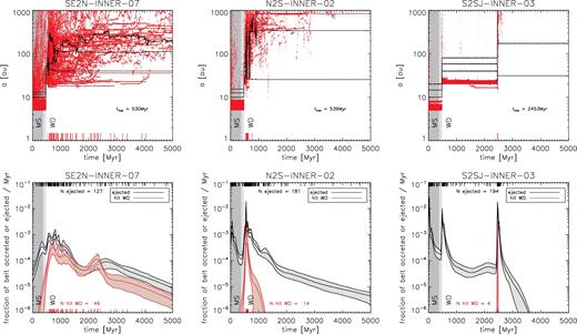
Time evolution of some example systems. Top row: Planets’ semi-major axes are marked in black, planetesimals’ in red. Large ticks at the bottom axis mark where test particles collided with the WD. The time at which orbit-crossing begins, measured from the zero-age MS, is shown on the plot. Left-hand panel: se2n example. This is the run that resulted in the greatest number of planetesimals hitting the WD (46 in all). Scattering amongst the planets begins around 50 Myr after the star becomes a WD (total age 530 Myr), but all three planets remain bound for the duration of the simulation. This allows material to be delivered to the WD for several Gyr, albeit at a decreasing rate. Centre: n2s example. An instability among the planets soon after mass loss results in delivery of material to the WD over a period of a few hundred Myr. Following ejection of one of the planets, remnant belt particles are slowly cleared, but none at these late times collide with the WD. Right-hand panel: s2sj example. Here, we see a widening of the chaotic zone and ‘Kirkwood gaps’ along the MS, a further broadening of the chaotic zone following mass loss, and then an instability among the planets just before 2.5 Gyr. This rapidly depletes the rest of the belt, and causes a small amount of material to be delivered to the WD. The final system comprises two planets and no test particles. Bottom row: Kernel density estimates of times at which planetesimals hit the star or are ejected, with times marked as large tick marks on the upper and lower axes. The rate at which particles are lost increases dramatically following stellar mass loss and the onset of orbit-crossing amongst the planets.
These four phases are particularly evident in the right-hand panels of Fig. 6. Rates of ejection begin high, and fall as the unstable regions of the belt are cleared along the MS. Ejections spike and fall again after the star becomes a WD. At around 2.4 Gyr, the planets undergo a short-lived instability resulting in the ejection of one of them. During and after this, ejection rates again peak and decay, and a handful of particles collide with the WD.
3.2 Particles colliding with the WD
We now turn our attention to the particles colliding with the WD, and the times at which this occurs. The numbers of particles directly hitting the WD in each simulation set, as well as the number crossing the Roche limit, are shown in Table 3. This table also shows the number of the particles remaining in the integration when the star became a WD, the number that survive to the end of the integration, and the fraction of the belt surviving when the WD formed that later collided with the WD. Two trends are clear from this table: Particles in the inner belts are more likely to hit the star than particles in outer belts, and the lower mass planets are much more efficient at causing accretion as opposed to ejection of particles. Ejection and collision with the star were the dominant loss channels after the star became a WD: Only 21 particles across all simulations struck one of the planets after the star became a WD.
Here, we consider the statistics of particles directly hitting the WD; as we shall discuss in Section 3.2.4, particles cross the Roche limit at a higher rate but with the same qualitative trends. Kernel density estimates of the times at which particles are lost to stellar collision or ejection in three example integrations are shown in the lower panels of Fig. 6. Both the number of particles hitting the star and the time-scale over which this delivery is maintained increase as the mass of the planets decreases. To explore the rates of delivery as a function of time in a population of systems, all the integrations in each simulation set are then combined to give Fig. 7. Here, the upper panels show the absolute times at which particles were lost, whereas the lower panels show times relative to the onset of orbit-crossing among the planets. We also show for comparison the trend in the upper envelope of accretion rates from the DZ sample of Hollands et al (submitted), which decays exponentially with an e-folding time of 0.95 Gyr; additionally, we show an accretion rate of 109 g s−1 from a 1 M⊕ belt, at the high end of WD accretion rates (Koester et al. 2014). We now discuss the simulation sets in more detail.
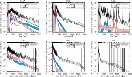
Top row: Kernel density estimates of the times at which test particles hit the star or are ejected from the system. Ejections are summed across all integrations in a given set; stellar collisions are divided according to whether the particles originate in an inner or an outer belt. The actual times of ejection are marked on the upper horizontal axis as black ticks; times of stellar collision are marked on the lower horizontal axis with red ticks (if from the inner belt) or purple ticks (if from the outer belt). We also show as a horizontal dotted line an accretion rate of 109g s−1 for a 1 M⊕ belt. The solid green line shows the observational trend (with arbitrary normalization) from Hollands et al (submitted) for late cooling ages of over 1.5 Gyr, together with its extrapolation to younger cooling ages. Bottom row: As above, but showing the time of ejection/collision after planetary instability (orbit-crossing) begins: Each system is separately translated so that its orbit crossing begins at t = 0, and then the kernel density estimate is constructed. Vertical lines mark the durations of individual simulations past the onset of orbit crossing.
3.2.1 Saturn to super-Jupiter
These runs saw the lowest numbers of particles colliding with the WD, with only 11 from the outer belts and 25 from the inner belts being lost this way, representing, respectively, |$0.6\,\,\rm{per\,\,cent}$| and |$2.3\,\,\rm{per\,\,cent}$| of the particles surviving at the onset of the WD phase.
Times at which particles strike the WD range from cooling ages of 300 Myr to 4.4 Gyr.4 Although this gives a respectable range, in any one simulation the accretion events usually occur in a relatively brief window of a few 10s of Myr following instability among the giant planets, as can be seen in the lower right-hand panels of Figs 6 and 7. Hence, instability among giant planets is unlikely to allow ongoing accretion for 100s of Myr to Gyr throughout the WD lifetime.
3.2.2 Neptune to Saturn
The intermediate-mass systems were much more efficient at delivering material to the WD. A total of 85 particles from the outer belts and 190 from the inner belts struck the WD, representing, respectively, |$5.4\,\,\rm{per\,\,cent}$| and |$12.1\,\,\rm{per\,\,cent}$| of the particles surviving at the onset of the WD phase.
The time of the instability amongst the planets in these simulation was not so variable as in the s2sj set. Compared to the more massive planets, run n2s shows a broader peak in the distribution of times of delivery. Sporadic ejections continue for several Gyr. However, the accretion is still restricted to a relatively brief window of a few 100 Myr during and after instability (centre panels of Figs 6 and 7).
3.2.3 Super-Earth to Neptune
These runs were the most efficient at delivering particles to the WD, with 138 particles from outer belts and 286 from inner belts colliding with the WD, representing, respectively, |$7.7\,\,\rm{per\,\,cent}$| and |$17.1\,\,\rm{per\,\,cent}$| of the particles surviving at the onset of the WD phase.
This run shows a still broader distribution of delivery times (left-hand panels of Figs 6 and 7). Delivery is maintained even at late times of several Gyr (measured both absolutely and with respect to the onset of planetary instability), although the rate does slowly decay. High rates of ≳ 10−5 of the belt per Myr are maintained for the first 2 Gyr after instability. This rate represents ∼2 × 10⁹ g s−1 for a belt of 1 M⊕. The rate of decay in the upper envelope of observed accretion rates at late times found by Hollands et al (submitted) is matched very well by the simulations with outer belts, whereas the inner belts have an accretion rate that falls off a little more steeply. Both of the belt configurations agree much more closely with the observed trend than do any of the configurations with higher-mass planets.
3.2.4 Collision with the WD versus tidal disruption
Hitherto, we have considered a conservative condition for the accretion of material on to the WD: the physical collision between a particle and the star. However, the physical radius of the WD is smaller, by a factor of ∼100, than the Roche limit at which bodies are tidally disrupted. Bodies with pericentres smaller than this distance (roughly 1 Solar radius, depending on density) will be shredded into long debris trails (e.g. Debes et al. 2012; Veras et al. 2014). An optimistic condition for accretion on to the WD would be to assume that all material entering this Roche limit would be accreted. Thus, direct collision and entry inside the Roche limit should bracket the true amount of material accreted.
We show in the final two columns of Table 3 the total number of particles entering within 0.003 au of the WD, together with the fraction of the belt surviving the AGB that this represents. These values are considerably higher than those for the number of particles colliding with the WD: |$4.7\,\,\rm{per\,\,cent}$| and |$13.3\,\,\rm{per\,\,cent}$| for the s2sj sets with outer and inner belts, respectively, compared to |$0.7\,\,\rm{per\,\,cent}$| and |$2.3\,\,\rm{per\,\,cent}$| for the particles actually hitting the WD. With the less massive planets, these values are |$20\,\,\rm{per\,\,cent}$| and |$37\,\,\rm{per\,\,cent}$| from the outer and inner belts. Interestingly, the n2s and se2n sets are equally efficient at driving material inside the Roche limit, in contrast to their efficiencies at delivering material to the WD radius where the se2n simulations perform better. The fraction of belt material delivered to the Roche limit and the WD radius in the different simulation sets is displayed graphically in the upper panel of Fig. 8.
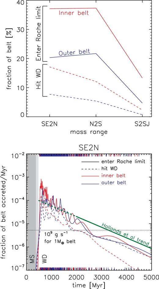
Top row: Accretion efficiency on to the WD in our simulations. The horizontal axis shows the mass range of the planets: se2n ‘super-Earth to Neptune’; n2s ‘Neptune to Saturn’, and s2sj ‘Saturn to super-Jupiter’. On the vertical axis is plotted the fraction of the belt which survived AGB evolution which later enters the WD's Roche limit (0.003 au, solid lines) or collided with the WD (5 × 10⁻⁵ au, dashed lines). The red and blue lines mark simulations with inner and outer belts, respectively. The efficiency of delivery increases with decreasing planet mass. Bottom row: Rates of delivery to the Roche limit (solid) and the WD radius (dashed) in our se2n runs. Red and blue lines mark simulations with inner and outer belts, respectively. Despite the higher efficiency with which material is delivered to the Roche limit compared to the WD surface, the trend with time is the same.
Material is delivered to the Roche radius at higher rates than it is delivered to the WD surface, as is to be expected since not all particles crossing the Roche limit will have their pericentres forced down to the WD radius itself. However, the trend in accretion rate with time, as measured by the rate at which material reaches these two thresholds, is broadly similar, as can be seen in the lower panel of Fig. 8 for the se2n simulations. At very late times, the accretion rate from the inner belts does not fall off as steeply when using the Roche limit as a threshold compared to when using the WD radius, and better matches the observed decay rate from Hollands et al (submitted). In the n2s and s2sj sets, the time over which material is delivered to the Roche limit is brief.
What is the fate of the material that crosses the Roche limit? In pure dynamical terms, some fraction of it does later collide with the WD: |$17\,\,\rm{per\,\,cent}$| in the s2sj runs, |$30\,\,\rm{per\,\,cent}$| in n2s, and |$43\,\,\rm{per\,\,cent}$| in se2n. These bodies will constitute the ‘steeply infalling debris,’ whose destiny was studied by Brown et al. (2017). The remainder may undergo circularization and collisional processing (e.g. Veras et al. 2015; Kenyon & Bromley 2017). Before these processes occur, however, the bodies may be ejected, particularly when the planets are massive. In the s2sj runs, |$82\,\,\rm{per\,\,cent}$| of bodies that crossed the Roche limit were subsequently ejected from the system, with a median lifetime to ejection of only 18 Myr. As planet masses are reduced, ejection becomes less efficient and takes longer: In n2s, |$65\,\,\rm{per\,\,cent}$| of these bodies are ejected, with a median lifetime of 152 Myr, and in se2n only |$43\,\,\rm{per\,\,cent}$|, with a median lifetime of 677 Myr. Now, circularization of debris streams from disrupted bodies may take many Myr (e.g. Veras et al. 2015). We might expect therefore that much of the disrupted material in the s2sj systems does not, in fact, make it down to the WD surface but will continue to be scattered by the planets and be ejected into interstellar space. On the other hand, most of the disrupted material in systems with low-mass planets will not be scattered out of the system but will make its way to the surface of the WD, whether through circularization of the debris stream or ongoing gravitational interactions with the planets.
A final caveat here is that, for computational reasons, we did not include GR corrections in the numerical integrations. These will in general hinder the delivery of material to the WD, as they can suppress secular eccentricity forcing such as through the Kozai mechanism. The final delivery of material even by the low-mass planets may therefore be achieved not through purely dynamical forcing from the planets but by other forces acting to circularize the debris streams.
3.2.5 Accretion at early WD cooling ages
Scattering following instabilities amongst low-mass planets well reproduces the trend in accretion at late times. We now consider accretion at young WD cooling ages of ∼100 Myr. Koester et al. (2014) studied young DA WDs and found that accretion only became detectable at cooling ages of a few 10s of Myr. In Fig. 9, we show the inferred mass accretion rates from detections of atmospheric Si (Koester et al. 2014) and Ca (Koester & Wilken 2006), where we assumed a modest belt mass of 10−3 M⊕. Interestingly, the observational detections begin at exactly the ages at which delivery of material to the WD begins in our se2n simulations. The first particle to cross the Roche limit did so at a cooling age of 39 Myr, and the first to strike the WD did so at a cooling age of 56 Myr. Following this, the rate of delivery increased rapidly to a plateau, as shown in Fig. 9. The lack of accretion at young ages is partly due to the delay after stellar mass loss before orbit-crossing begins and partly due to the delay in delivering material to the WD once the planetary instability begins: The earliest delivery of a particle to the WD in the se2n runs was 16 Myr after the onset of orbit crossing. Thus, even if our planetary system had been slightly less widely separated, so as to induce instabilities as soon as possible after stellar mass loss, there would still have been a delay in the delivery of material to the WD. Scattering amongst low-mass planets therefore correctly reproduces the trends in accretion rates on to young WDs as well as old. We caution that Koester et al. (2014) pointed out that the route from disruption to accretion may be different around these younger, hotter, WDs, which may result in accretion occurring in shorter, more intense bursts with a low duty cycle.
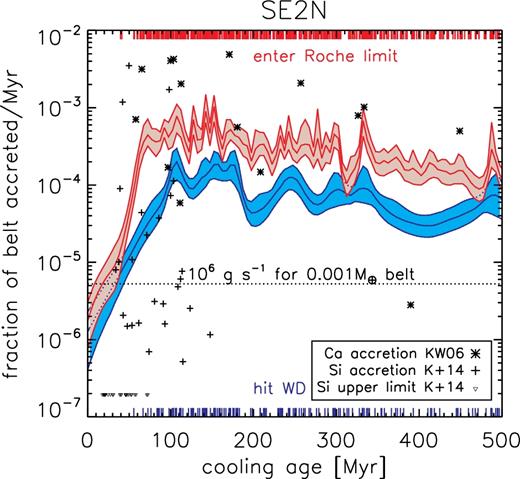
Accretion rates around young WDs. Here, both inner and outer belts from the se2n simulations are combined, and the colours indicate the rates at which particles cross the WD's Roche limit (red) or collide with the WD (blue). No particles are delivered at young ages, with particles beginning to cross the Roche limit at ∼40 Myr. This is approximately the age at which accretion rates become detectable in the young DA sample of Koester et al. (2014). The data from Koester et al. (2014) are shown as crosses (Si-accreting systems) and triangles (upper limits), and data from Koester & Wilken (2006) as stars (Ca-accreting systems). Conversion of the observed accretion rates to our y-axis assumes a belt mass of 10−3 M⊕ and a conversion of the elemental mass to the bulk Earth.
Surprisingly, we found almost no accretion in the systems prior to planetary orbit-crossing. Our simulations, integrating from the beginning of the MS through AGB mass loss to eventual planetary instability, naturally include the growth of chaotic regions associated with mean-motion resonances with the planets, even before the planets begin significantly exciting each other's eccentricities as orbit-crossing begins. We found that the growth of these chaotic regions, however, does not result in accretion on to the WD: Across all simulations, one single particle crossed the WD's Roche limit (and was subsequently ejected) before planetary orbit-crossing began. This was located in the inner belt close to the 2:1 resonance with the innermost planet in one of the s2sj runs, and survived a few 10s of Myr beyond the formation of the WD before beginning to experience large eccentricity excursions. This single particle represents a very low efficiency of pollution (|$0.09\,\,\rm{per\,\,cent}$| of the inner belt particles surviving the AGB). We discuss this issue further in Section 4.2.
3.2.6 Orbital inclinations of bodies accreted on to the WD
In our integrations, we recorded the final position and velocity of objects colliding with the WD, allowing the instantaneous orbital inclination (with respect to the original reference plane of the planetary system) to be determined. Bodies approaching the WD come in with a roughly isotropic distribution of orbital inclinations (Fig 10, top panel). This has several consequences. First, in systems exhibiting transiting asteroids such as WD 1145+017, we might not expect any correlation between the orbital inclination of the asteroids or disc and the inclinations of scattering bodies in the outer system. Secondly, we should not expect any correlation between the orbital planes of successively infalling bodies in any one system – and indeed, the orbital planes of the asteroids of WD 1145+017 (edge-on) and the dust disc (not edge-on, as required to present a large enough emitting surface) probably have some mutual inclination (Xu et al. 2018). The lower panel of Fig 10 shows the time intervals between successive accretion events in the se2n runs, and the mutual inclinations of the orbits of successive infalling bodies. The mutual inclination distribution is again isotropic, and no correlation is seen with the time between accretion events, although all of our events in the se2n runs are separated by at least 0.1 Myr.5 We also mark on some time-scales relevant for later evolution of the disrupted planetesimals around the WD: the time-scale for orbit shrinking tshr from Veras et al. (2015), for debris of mm and dm sizes, and the lifetime of circumstellar dust discs (which are not undergoing the faster runaway accretion) from Rafikov (2011). Note however that the disc lifetimes are highly uncertain: Metzger, Rafikov & Bochkarev (2012) estimated lifetimes of 1–10 Myr, similar to Rafikov (2011), whereas semi-empirical analyses by Jura (2008) and Girven et al. (2012) argued for slightly shorter lifetimes of 0.01–1 Myr. Time-scales of ≳1 Myr imply that in many cases the infalling planetesimals will meet tidal streams from previous disruption events in the process of circularization, or circularized material now forming a disc of gas and dust round the WD (Jura 2008; Wilson et al. 2014). The high mutual inclinations mean that significant collisional processing, at very high velocities, will occur for the infalling material. Collisional damping at the high velocities in the neighbourhood of the WD is expected to be weak (Kenyon & Bromley 2017), and so these high inclinations will be maintained as collisions occur. Significant collisional vapourization of this material can therefore be expected.
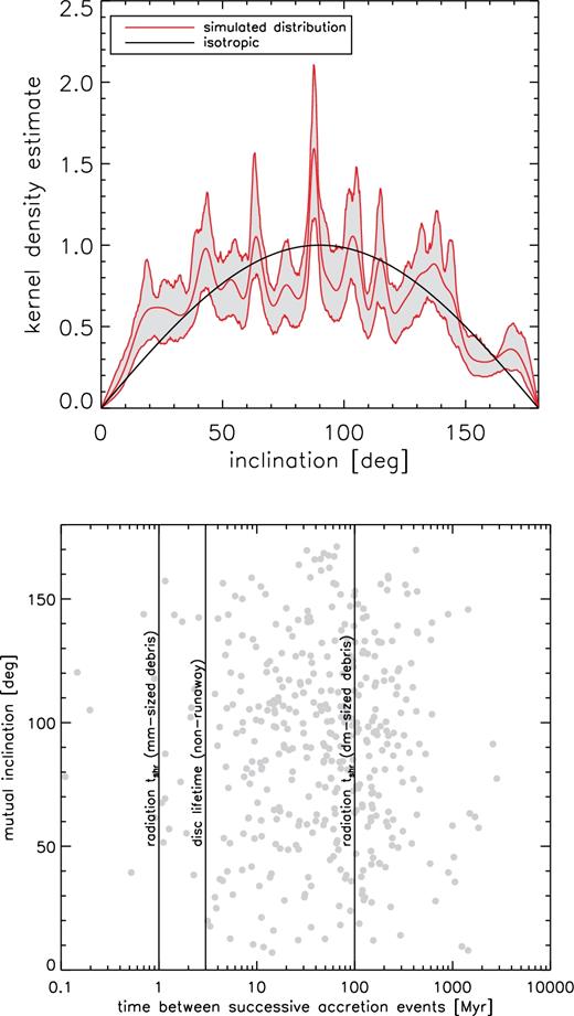
Top row: Orbital inclinations, with respect to the original reference plane, of test particles removed upon colliding with the WD, in all the se2n runs. The distribution is isotropic, with a weak excess at near-polar inclinations. Bottom row: Intervals between successive accretion events (here defined as striking the WD) and mutual orbital inclinations of successive accreted planetesimals. The distribution of these mutual inclinations is again isotropic, and no correlation with the interval between events is seen. Vertical lines show the approximate durations of two successive phases leading to WD pollution: the approximate lifetimes of debris belts circularizing under radiation forces (from Veras et al. 2015, for two particle sizes) and the expected lifetime of circumstellar dust discs (from Rafikov 2011, but there is considerable uncertainty in these estimates, e.g. Girven et al. 2012).
4 DISCUSSION
4.1 Current observations of prevalence and rates of accretion
At least |$25\,\,\rm{per\,\,cent}$| of WDs show spectroscopic evidence of metal pollution (e.g. Koester et al. 2014). If WD pollution is to be attributed largely to one dominant dynamical mechanism arising from one dominant system architecture, this architecture must therefore be found around a significant fraction of stars. In this sense, planets with masses in the super-Earth range are good candidates for being the perturbers that drive the accretion of material on to WDs. In the region probed by RV and transit surveys, within 1 au around Solar-type stars, the planetary occurrence rate rises steeply towards smaller planets, and several 10s of per cent of stars host at least one super-Earth or Neptune (Mayor et al. 2011; Fressin et al. 2013). This region will be totally cleared of planets by the star's RGB and AGB evolution (Villaver & Livio 2009; Mustill & Villaver 2012; Villaver et al. 2014). However, if these occurrence rates also apply to planets at ≳5 au around intermediate-mass stars, low-mass planets are immediately more promising as a driver of pollution than are systems of unstable gas giants.
The main weakness here is that for pollution to occur the planetary orbits themselves are required to be destabilized by AGB mass loss: Recall that across all simulations we found only one single planetesimal that crossed the WD's Roche limit before planetary orbit-crossing began. As we showed in our preliminary simulations, the systems of super-Earths must be separated by ∼6–10 mutual Hill radii to favour stability on the MS followed by instability after the star becomes a WD (Table 1 and Fig. 3). If we continue our use of known close-in systems as an analogy for the wider systems orbiting WD progenitors, we must note that the typical multiplanet system discovered by Kepler has a separation of ∼10–30 mutual Hill radii (Weiss et al. 2017), which would imply that most systems probably remain stable following AGB mass loss. Alternatively, one could be optimistic and predict that the planetary systems orbiting intermediate-mass stars have a tighter spacing than those found on close orbits around Solar-type stars. From Table 1, we see that a pollution occurrence rate of |$25\,\,\rm{per\,\,cent}$| could be attained if all intermediate-mass stars have multiple super-Earths at ∼10 au, and they are separated by ∼10 mutual Hill radii.
The time dependence of the accretion rates is an important test for evaluating mechanisms of WD pollution. Hollands et al (submitted) have recently measured WD accretion rates in a sample of old DZ WDs, with cooling ages from 1 to 8 Gyr, allowing a comparison of our simulation results with an observational sample spanning a large range of cooling ages. They find an exponential decay in the accretion rates with age, with an e-folding time of 0.95 Gyr. This trend is overplotted in the upper panels of Fig. 7 and the lower panel of Fig. 8. A very good match to the se2n simulations is seen, particularly those with outer planetesimal belts. Those with inner belts show a decay that is a little steep at late times, although this discrepancy disappears if we use passage of the Roche limit, rather than collision with the WD, as a criterion for accretion (Fig. 8). In contrast, the more massive planets in simulations n2s and s2sj both result in bursts of accretion that end very soon after instability. Moreover, very few planetesimals are left following instability among high-mass planets, so such systems experiencing an instability will not have a reservoir of planetesimals to draw on should they also host lower mass planets. This means that the observed pattern of WD pollution rates is inconsistent with large numbers of intermediate-mass stars hosting unstable systems of giant planets (consistent with direct imaging surveys of A-type stars; Vigan et al. 2017), but it is consistent with large numbers hosting unstable systems of super-Earths. As we discussed above, this is believable in light of planetary occurrence rates around Solar-type stars.
The observed time dependence of accretion rates on to young WDs is a second important constraint. Koester et al. (2014) found no detectable accretion on to DA WDs younger than a few 10s of Myr, after which the accretion was detected. This was not an observational bias as the upper limits for the younger WDs are below the detected rates around the older WDs. This is a second observational trend that our se2n simulations successfully reproduce (Fig. 9). The first particle to cross the Roche limit in our simulations did so at a cooling age of 39 Myr, whereas the first to directly collide with the WD did so at 56 Myr. After this, accretion rates quickly reach a plateau and then begin the slow decay discussed above.
The final consideration is the absolute scaling of the accretion rates. The accretion rates inferred from spectroscopic observations of WDs range from ∼105 to 109 g s−1 (e.g. Koester et al. 2014), or ∼5 × 10⁻¹⁰ − 5 × 10⁻⁶ M⊕ Myr−1. Let us take 109 g s−1 as a high accretion rate. If this were to be maintained in a system for 5 Gyr, it would imply a total of |$0.026\, \mathrm{M_{{\oplus}}}$| of material delivered in total in this time. If low-mass planets deliver material to the WD with |${\sim }20\,\,\rm{per\,\,cent}$| efficiency, this implies a total belt mass of ∼0.13 M⊕. This can be compared with the Solar system's Asteroid Belt mass of 5 × 10⁻⁴ M⊕ (Pitjeva 2005): At |$20\,\,\rm{per\,\,cent}$| efficiency, our Asteroid Belt could maintain a delivery rate of ∼2 × 10⁷ g s−1 over 5 Gyr. We note that these relatively low belt masses (≲1 M⊕) mean that our use of massless test particles to model the planetesimals is valid, since the dynamical friction they impose on the planets in the system will be negligible (see Appendix B).
Higher accretion rates, if they are not transient, require higher belt masses, and there is a limit to the amount of material that can be present in a planetesimal belt set by collisional evolution: belts that are initially more massive experience faster collisional evolution and at late times the belt mass tends asymptotically to the same level, regardless of the initial mass (Wyatt et al. 2007). For 3 M⊙ progenitors, Bonsor & Wyatt (2010) estimated that a belt centred at 10 au and of width 5 au should only preserve 10−4 M⊕ of material to the end of the AGB, although this estimate assumed a maximum planetesimal size of 2 km. The maximum permitted belt mass is linearly proportional to the maximum planetesimal size and so belts containing larger planetesimals of a few hundred km in radius should be able to support the highest accretion rates of ∼109 g s−1.
More distant belts experience much slower collisional evolution: For a fixed ratio of belt width Δr to radius r, the collision time-scale and maximum belt mass scale as r13/3. Despite the lower efficiency of delivery from the more distant outer belts, the increased mass reservoir they support means that they can support higher accretion rates. However, recall the compositional constraint introduced in Section 1: Few polluted WDs show evidence for significant quantities of water. This implies that most source material originates relatively close to the star. Recent work by Malamud & Perets (2017b) has found that bodies of 100 km in size orbiting initially at 10 au around a 3 M⊙ progenitor will be depleted of water on the AGB, whereas larger or more distant bodies will retain some fraction (Malamud & Perets 2017a).
This implies that the inner belts in our simulations should be entirely water-depleted except for the largest, rarest bodies, and so our inner belt simulations match the observational constraints from the point of view of composition as well as the rate of accretion and its time dependence.
4.2 Comparison of rates from this paper to other proposed mechanisms
We now compare the accretion rates determined in this paper to those calculated in other scenarios. Frewen & Hansen (2014) found very high accretion efficiencies for a single eccentric planet embedded in a planetesimal belt, approaching 100 per cent of unstable belt particles being accreted on to the star for low-mass (10 M⊕), eccentric (e = 0.8) planets, at a rate of 7 × 10⁻⁵ of the unstable belt mass per Myr at a cooling age of 1 Gyr. This fractional rate is comparable to the rates we attain at a similar time in our se2n simulations. As we argued above, this is sufficient to reproduce the observed accretion rates. The advantages our model have over that of Frewen & Hansen (2014) are: self-consistent dynamical modelling to explain the presence of such an eccentric planet in a disc of planetesimals; the ability to destabilize a wider annulus of planetesimals, meaning a greater mass reservoir; and a larger semi-major axis, allowing more mass to survive collisional grinding on the MS.
The pre-instability phase of our simulations encompasses two related phenomena studied as potential mechanisms of WD pollution in previous works: The expansion of the chaotic zone of resonance overlap surrounding a planet's orbit (Wisdom 1980; Bonsor et al. 2011; Mustill & Wyatt 2012) and the expansion of individual unstable mean motion resonances (Debes et al. 2012). Bonsor et al. (2011) studied an outer belt surrounding a single planet on a circular orbit. They were able to obtain high accretion rates of 109–1010 g s−1, but only on the assumption that material could be efficiently transported to the WD after scattering: With a single planet, particles did not attain pericentres less than 0.3 times the planetary semimajor axis. Further transport requires extra planets in the system. We did not find any particles transported to the Roche limit from our outer belts in our three-planet simulations prior to planetary instability. This is not surprising, since further work by Bonsor et al. (2012) found that higher-multiplicity systems are required to deliver material even to ∼1 au.
It is perhaps more surprising that we did not see a significant contribution from the 2:1 interior MMR. Debes et al. (2012) showed that, in the case of the Solar system, this unstable resonance with Jupiter will broaden following AGB mass loss and provide a source of material to pollute the WD, with |${\sim }2\,\,\rm{per\,\,cent}$| of their modelled asteroids crossing the WD's Roche limit. In contrast, we found only one such disrupted body, in the s2sj runs, accounting for only |$0.9\,\,\rm{per\,\,cent}$| of that belt, or |$0.1\,\,\rm{per\,\,cent}$| over all 10 simulations of inner belts. A large amount of this discrepancy can be attributed to our distribution of particles, which was much broader (3.5 au in the s2sj-inner runs) than the source region around the 2:1 resonance most relevant for the delivery mechanism of Debes et al. (2012) (which would be 0.6 au for our belt radius). Thus, only 17 per cent of our belt is located around the 2:1 MMR. If we apply the 2 per cent survival rate from Debes et al. (2012) to 17 per cent of the belt particles surviving to the AGB tip (1069 across all s2sj-inner runs), we expect 3.6 particles to enter the WD Roche limit prior to planetary instability. This is consistent with our single disruption (the probability of seeing 0 or 1 disruptions with a Poisson rate of 3.6 is |$12.6\,\,\rm{per\,\,cent}$|).
With such small number statistics, we cannot say definitively that our simulations are less efficient at delivery from the 2:1 MMR. However, there are reasons to suspect that they should be. Recall that, in the Solar system, the unstable resonances are cleared by secular resonances and by secondary resonances between the frequency of the mean motion resonance itself and other frequencies in the system, with the 2:1 being cleared by a secondary resonance between the resonant libration period and the apsidal period whose efficiency depends upon the eccentricities and masses of Jupiter and Saturn (Lecar et al. 2001). Perhaps our Solar system's Kirkwood Gaps are unusually efficient at delivering material to the Roche limit, or the systems we integrated in this paper unusually inefficient. In particular, the eccentricities of the planets prior to instability are about an order of magnitude lower in our simulations than the eccentricities of Jupiter and Neptune. This has a strong effect on the stability of orbits in Jupiter's 2:1 MMR (see fig. 7 of Lecar et al. 2001).
A final possibility is that the difference in disruption rates is an artefact of the choice of integrator used. We have used RADAU for the integrations in this paper, whereas Debes et al. (2012) used Bulirsch–Stoer. We also ran the s2sj-inner simulations with a Bulirsch–Stoer integrator, finding two particles crossing the WD's Roche limit prior to planetary orbit-crossing. Given the small number statistics, we do not have enough evidence to claim a systematic difference between the RADAU and BS integrators in this specific case.
5 CONCLUSIONS
We show, in self-consistent N-body integrations lasting throughout a star's life, that planet–planet scattering in the presence of a planetesimal disc can provide ongoing accretion on to the WD for several Gyr.
Planet–planet scattering triggered by post-MS stellar mass loss provides a natural way of generating the eccentric planetary orbits that are optimal for efficient delivery of planetesimals to the WD. Following scattering, planetary eccentricities remain high, since the planetesimal disc masses required to explain observed accretion rates are not high enough for significant dynamical friction.
Low-mass planets (super-Earth to Neptune) are highly efficient at delivering material, and this delivery is ongoing, albeit at a decreasing rate, for several Gyr (Fig. 7). The decay rate is similar to that recently measured in DZ WDs (Hollands et al., submitted).
Low-mass planetary systems also reproduce the observed delay of a few 10s of Myr before the onset of accretion on to a newborn WD (Koester et al. 2014, and Fig. 9).
Instabilities in systems of Jovian planets result in little accretion, and this is confined to a narrow window of a few 10s of Myr.
Low-mass gas giants (Neptune to Saturn) deliver a larger fraction of the belt to the WD than do higher mass giants, but pollution remains confined to a brief time window of a few hundred Myr.
The ability of the scattering planets to sweep up material from a relatively wide belt ensures a large mass reservoir that can provide sufficient material to explain the observed accretion rates.
Material accreted on to the WD has a roughly isotropic distribution of orbital inclinations (Fig. 10). Thus, scattered asteroids are likely to meet other asteroids, debris streams, or discs at high mutual inclinations. Significant collisional processing – fragmentation and vapourization – of material may therefore take place before it is finally accreted on to the WD.
The main challenge to our model comes from the unknown distribution of planetary separations prior to planetary instability. We find that planets separated by 6–10 mutual Hill radii on the MS will mostly survive MS evolution and become unstable after mass loss (Table 1, Fig. 3). If the wide-orbit low-mass planets we require are more widely separated, however, the incidence of planetary instability may be insufficient to explain the prevalence of WD pollution. On the other hand, if planet–planet scattering is indeed responsible for the pollution of WDs, we predict that a large fraction |${\gtrsim }30\,\,\rm{per\,\,cent}$| of WD progenitors will have close-packed systems of super-Earths at presently undetectable separations of ∼10 au.
ACKNOWLEDGEMENTS
AJM is supported by the project grant 2014.0017 ‘IMPACT’ from the Knut & Alice Wallenberg Foundation. This work has benefited from computer hardware and travel funds from the Walter Gyllenbergs fund of the Royal Physiographic Society in Lund. EV acknowledges support from the Spanish Ministry of Economy and Competitiveness (MINECO) under grant AYA-2014-55840P. BTG received funding from the European Research Council under the European Union's Seventh Framework Programme (FP/2007–2013)/ERC Grant Agreement n. 320964 (WDTracer). DV gratefully acknowledges the support of the Science and Technology Facilities Council via an Ernest Rutherford Fellowship (grant ST/P003850/1). AB acknowledges the support of the Royal Society by a Dorothy Hodgkin Fellowship. We thank Mark Hollands for providing the data on DZ pollution rates, and Jay Farihi, Jeremy Heyl and the anonymous referee for comments that improved the paper.
Footnotes
For stars of this mass, the AGB tip radius of ∼3 au is considerably larger than the maximum RGB radius of ∼0.2 au.
In this paper we show kernel density estimates constructed with an adaptive-width (k-nearest neighbour) Gaussian kernel (Feigelson & Babu 2012). The adaptive width resolves abrupt features, such as the sudden increase in events after mass loss, while smoothing over regions of lower density such as the tail at later times.
This partly reflects the highly chaotic original system, whose stability lifetime is sensitive to the changes to the integrator timestep induced by the test particles.
The n2s runs saw two events separated by <1000 yr, with a mutual inclination of 160°.
REFERENCES
APPENDIX A: INTEGRATOR PERFORMANCE
Here, we briefly describe the integrator used for the simulations in this paper. A more complete description will be provided in Mustill et al (in preparation).
We adapt the RADAU integrator (Everhart 1985) from the Mercury software package (Chambers 1999). Unlike the fixed-time-step hybrid symplectic integrator, RADAU can accurately handle eccentric orbits (see, e.g. fig. 5 of Rein & Spiegel 2015), a necessity for studying the delivery of material to the WD Roche limit or surface. Unlike BS, which uses a modified midpoint method, the RADAU integrator is a predictor-corrector method, which utilizes Gauß–Radau spacings. Rein & Spiegel (2015) present an analysis of the performance of a (slightly modified) RADAU integrator compared to BS and symplectic algorithms, for the case of no mass loss. We modify the RADAU integrator to adjust the stellar mass and radius, fed in from an input file. As we showed with the BS integrator described in Veras et al. (2013a), it is essential to update the stellar mass not only at each major integrator time-step, but also at the subdivisions of these time-steps. This is done by linearly interpolating the mass and radius between the values recorded in the stellar evolution file.
We found that the modified RADAU integrator exhibits considerably better convergence properties than the BS integrator. In Fig. A1, we show the mean longitude of a planet initially at 10 au in a single-planet system at three times into the integration: 200 Myr (roughly halfway to the AGB tip), 500 Myr (after the AGB tip), and 5000 Myr (the end of the integration). These are plotted as a function of the stepwise error tolerance parameter. RADAU exhibits good convergence properties, with little difference in the final mean longitude for tolerance between 10−16 and 10−12, and only a small drift in final mean longitude for more lax tolerances. In contrast, BS only converges to the RADAU solution in a narrow tolerance range around 10−15, and the final mean longitude is essentially random for tolerances laxer than 10−13. RADAU is more computationally expensive than BS, and in this paper we adopt a tolerance of 10−11 as a compromise between speed and accuracy (this is |$25\,\,\rm{per\,\,cent}$| faster than running at a tolerance of 10−12). Although there is a small phase error by 5 Gyr at this accuracy, it is negligible at 500 Myr, a time more relevant for most of the dynamics.
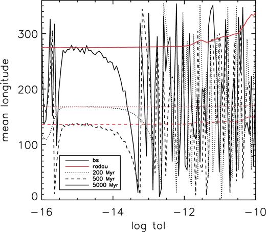
Performance of the RADAU integrator (adopted for this paper) compared to the BS integrator. We show the mean longitude of the planet of a single-planet system as a function of integrator tolerance, at three times: 200 Myr, 500 Myr (just after mass loss), and 5 Gyr. RADAU exhibits excellent convergence, whereas BS cannot accurately track the mean anomaly except in the narrow range of tolerances around 10−15.
APPENDIX B: IMPORTANCE OF ECCENTRICITY DAMPING
We test the extent to which eccentricity damping may affect the ability of a highly eccentric planet to scatter particles. We consider a set-up similar to that of Frewen & Hansen (2014), with a planet of eccentricity e = 0.8 embedded in a disc of planetesimals on circular orbits. We take 476 planetesimals, with a total mass of 1 M⊕. The planetesimals are massive test particles in Mercury: they interact gravitationally and collisionally with the planet and the star, but not with each other.
The 10 M⊕ planet's eccentricity falls approximately 10 per cent in the first 0.2 Myr (see Fig. B1). In contrast, the 1 M⊕ planet's eccentricity undergoes several damped secular cycles before stabilizing at 0.2. This damping decouples it from the surviving disc particles, and far fewer are lost than with the higher-mass planet.
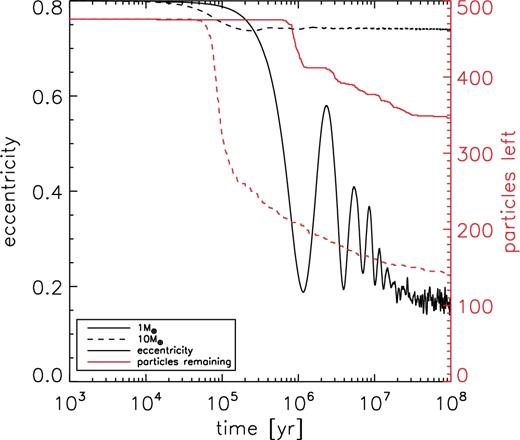
Systems of a single eccentric planet embedded in a disc of massive test particles. The total disc mass is 1 M⊕. When the planet is of comparable mass, strong eccentricity damping is seen, but only weak damping for a planet ten times more massive.
It is therefore safe to ignore eccentricity damping when the disc is only 10 per cent of the planet's mass, but not for comparable masses.
Author notes
STFC Ernest Rutherford Fellow.
