Cosmographic analysis with Chebyshev polynomials

Capozziello, Salvatore; D'Agostino, Rocco; Luongo, Orlando

doi:10.1093/mnras/sty422

Abstract

The limits of standard cosmography are here revised addressing the problem of error propagation during statistical analyses. To do so, we propose the use of Chebyshev polynomials to parametrize cosmic distances. In particular, we demonstrate that building up rational Chebyshev polynomials significantly reduces error propagations with respect to standard Taylor series. This technique provides unbiased estimations of the cosmographic parameters and performs significatively better than previous numerical approximations. To figure this out, we compare rational Chebyshev polynomials with Padé series. In addition, we theoretically evaluate the convergence radius of (1,1) Chebyshev rational polynomial and we compare it with the convergence radii of Taylor and Padé approximations. We thus focus on regions in which convergence of Chebyshev rational functions is better than standard approaches. With this recipe, as high-redshift data are employed, rational Chebyshev polynomials remain highly stable and enable one to derive highly accurate analytical approximations of Hubble's rate in terms of the cosmographic series. Finally, we check our theoretical predictions by setting bounds on cosmographic parameters through Monte Carlo integration techniques, based on the Metropolis-Hastings algorithm. We apply our technique to high-redshift cosmic data, using the Joint Light-curve Analysis supernovae sample and the most recent versions of Hubble parameter and baryon acoustic oscillation measurements. We find that cosmography with Taylor series fails to be predictive with the aforementioned data sets, while turns out to be much more stable using the Chebyshev approach.

methods: data analysis, dark energy, cosmology: theory

1 INTRODUCTION

The cosmic acceleration is today confirmed by a large number of observations (Riess et al. 1998; Perlmutter et al. 1999) and represents a consolidate challenge of modern cosmology. To disclose the physics behind it, model-independent techniques have been widely investigated during last years. Strategies towards model-independent treatments have as main target the determination of universe's expansion history without the need of postulating a priori dark energy contributions. A particular attention is currently given to cosmography (Saini et al. 2000; Visser 2004; Cattoën & Visser 2007; Arabsalmani & Sahni 2011; Cai & Tuo 2011; Capozziello, Lazkoz & Salzano 2011; Carvalho & Alcaniz 2011; Guimaraes & Lima 2011; Luongo 2011). Standard cosmography lies on Taylor expansions of cosmic distances. The method provides a powerful tool to study the dark energy evolution without assuming its functional form in the Hubble rate. Moreover, fixing limits over free cosmographic parameters alleviates degeneracy amongst models and enables to understand which paradigms are effectively favoured directly with respect to data surveys. Although cosmography candidates as a robust tool to understand whether dark energy evolves or not, cosmic data unfortunately span on intervals z ≥ 1. This limit poses severe restrictions on cosmography and makes inapplicable Taylor expansions built up around z ≃ 0.

One stratagem to overcome this problem is to parametrize Taylor expansions in terms of auxiliary variables. Unfortunately, even this case turns out to be jeopardized by severe error propagations over the final outcomes. More recently, a further effort has been the use of Padé approximation built-up to converge at higher redshift domains (Gruber & Luongo 2014; Wei, Yan & Zhou 2014). In this case, however, the expansion orders are not fixed a priori and this causes difficulties on evaluating the rate of convergence as z → ∞. Thus, the limits of standard Taylor approach lying on z ≥ 1 are essentially alleviated but not fully fixed.

Motivated by the need of reducing relative uncertainties in cosmography, we here propose a new cosmographic technique based on Chebyshev polynomials. Chebyshev polynomials represent sequences of orthogonal polynomials, recursively defined through trigonometric functions. In our approach, we develop a new Chebyshev cosmography adopting the strategy of building up rational approximations made by these polynomial functions. We demonstrate that, under the hypothesis of rational Chebyshev polynomials, distinguishing Chebyshev functions of first and second kinds is not relevant since the final output gives analogous results in both the cases. For simplicity, we limit our analysis on first kind Chebyshev polynomials only and we write the sequence of Chebyshev rational functions that better approximate Taylor series up to a certain order. We thus show that our Chebyshev ratios provide nodes in polynomial interpolation, minimizing cosmographic uncertainties leading to the most likely well-motivated approximation to cosmic distances. We even present theoretical motivations behind our choice by computing the convergence radii for different choices of polynomial approximations.

To check how well our model works, we also study Padé expansions and we compare the Chebyshev technique with them. We finally show the advantages of our procedure with respect to the old approaches using data surveys, confronting the cosmological quantities built from our method with the observables of the latest cosmological data sets. We adopt a Monte Carlo analysis employing the Metropolis–Hastings algorithm, choosing Joint Light-curve Analysis (JLA) supernova, baryon acoustic oscillation, and differential age measurements. We show the goodness of our procedures comparing the outcomes coming from standard cosmography and our method, showing that error uncertainties are effectively reduced.

The structure of the paper is as follows. In Section 2, we review the general aspects of cosmography. In Section 3, we describe the mathematical features of the Chebyshev polynomials and present the method of the rational Chebyshev approximations. In Section 4, we derive a new model-independent formula for the luminosity distance, and compare the new method with the standard cosmographic procedures to verify the goodness of our approach. In Section 5, we place observational limits on the cosmographic parameters through a confront with the most recent experimental data. Finally, in Section 6, we summarize our findings and conclude.

2 THE COSMOGRAPHIC APPROACH

The study of the cosmic evolution can be done independently of energy densities by means of cosmography. This model-independent technique only relies on the observationally justifiable assumptions of homogeneity and isotropy (Weinberg 1972; Visser 1997; Harrison 1976). The great advantage of this method is that it allows one to reconstruct the dynamical evolution of the dark energy term without assuming any particular cosmological model. Cosmography involves Taylor expansions of observable quantities that may, in principle, go up to any order. These expansions can be compared directly with data. The outcomes of this procedure ensure the independence from any postulated equation of state governing the evolution of the universe and, thus, help to break the degeneracy amongst cosmological models.

The homogenous and isotropic universe is governed by the single degree of freedom offered by a(t), as demanded by the cosmological principle. Hence, following the most recent measurements of Planck Collaboration XIII (2016) and assuming a spatially flat universe,¹ we can expand a(t) in Taylor series around present time t₀ (Visser 2005, 2015):

\begin{eqnarray} a(t)=1+\sum _{k=1}^{\infty }\frac{1}{k!}\frac{{\rm d}^k a}{{\rm d}t^k}\bigg | _{t=t_0}(t-t_0)^k \,, \end{eqnarray}

(1)

where a(t₀) = 1.

The expansion above defines the cosmographic series (Poplawski 2006, 2007; Cattoën & Visser 2008; Xu & Wang 2011; Aviles et al. 2012):

\begin{eqnarray} H\equiv \frac{1}{a}\frac{{\rm d}a}{{\rm d}t} \,, q\equiv -\frac{1}{aH^2}\frac{{\rm d}^2a}{{\rm d}t^2}, \end{eqnarray}

(2)

\begin{eqnarray} j \equiv \frac{1}{aH^3}\frac{{\rm d}^3a}{{\rm d}t^3} \,, s\equiv \frac{1}{aH^4}\frac{{\rm d}^4a}{{\rm d}t^4}, \end{eqnarray}

(3)

known in the literature as Hubble, deceleration, jerk, and snap parameters.² These coefficients are used to describe the expansion history of the universe at late times.

Using the relation z = a⁻¹ − 1 and equation (1), one finds the Taylor series expansion of the luminosity distance as function of the redshift (Demianski et al. 2012; Busti et al. 2015; Piedipalumbo, Della Moglie & Cianci 2015; Demianski et al. 2017):

\begin{eqnarray} d_L(z)&=&\frac{c}{H_0}z\big [1+\frac{z}{2}(1-q_0) -\frac{z^2}{6}\left(1-q_0-3q_0^2+j_0\right) \nonumber \\ &&+\,\frac{z^3}{24}\left(2-2q_0-15q_0^2-15q_0^3+5j_0+10q_0j_0+s_0\right) \nonumber \\ &&+\, \mathcal {O}(z^4)\big]. \end{eqnarray}

(4)

The above expression for the luminosity distance can be used to obtain limits on the cosmographic parameters and study the low-z dynamics of the universe with no need of any a priori assumed cosmological model. In fact, plugging equation (4) into the definition

\begin{eqnarray} H(z)=c\, \left[\frac{{\rm d}}{{\rm d}z}\left(\frac{d_L(z)}{(1+z)}\right)\right]^{-1}\,, \end{eqnarray}

(5)

one gets

\begin{eqnarray} H(z)&\simeq H_0\left[1+H^{(1)}z+H^{(2)}\frac{z^2}{2}+H^{(3)}\frac{z^3}{6}\right]\,, \end{eqnarray}

(6a)

\begin{eqnarray} H^{(1)}&=&1+q_0\,, \end{eqnarray}

(6b)

\begin{eqnarray} H^{(2)}&=&j_0-q_0^2\,, \end{eqnarray}

(6c)

\begin{eqnarray} H^{(3)}&=3q_0^2+3q_0^3-j_0(3+4q_0)-s_0\,, \end{eqnarray}

(6d)

which describes the expansion history of the late-time universe up to the snap parameter.

2.1 The convergence problem

The limits of the standard cosmographic approach, based on the Taylor approximations, emerge when cosmological data at high redshifts are used to get information on the evolution of the dark energy term. In fact, the Taylor series converges if z < 1, so that any cosmographic analysis employing data beyond this limit is plagued by severe restrictions. A way to extend the radius of convergence of the Taylor series to high-redshift domains is represented by the method of rational approximations, amongst which the Padé polynomials represent a relevant example (Baker & Graves-Morris 1996). The Taylor expansion of a generic function f(z) is |$f(z)=\sum _{i=0}^\infty c_i z^i$|⁠, where c_i = f⁽ⁱ⁾(0)/i!, whereas one defines the (n, m) Padé approximant of f(z) as the rational polynomial

\begin{eqnarray} P_{n,m}(z)=\frac{\displaystyle {\sum _{i=0}^{n}a_i z^i}}{1+\displaystyle {\sum _{j=1}^{m}b_j z^j}}\,. \end{eqnarray}

(7)

Since by construction one requires that b₀ = 1, we have

\begin{eqnarray} f(z)-P_{n,m}(z)=\mathcal {O}(z^{n+m+1})\,. \end{eqnarray}

(8)

The coefficients b_i in equation (7) are thus determined by solving the following homogeneous system of linear equations (Litvinov 1993):

\begin{eqnarray} \sum _{j=1}^m b_j\ c_{n+k+j}=-b_0\ c_{n+k}, \end{eqnarray}

(9)

valid for |$k=1,.... ,m$|⁠. All coefficients a_i in equation (7) may be computed using the formula

\begin{eqnarray} a_i=\sum _{k=0}^i b_{i-k}\ c_{k}\,. \end{eqnarray}

(10)

The technique of Padé approximations has been recently investigated in the context of cosmography to handle the divergence problems at high-z domains (Gruber & Luongo 2014; Wei et al. 2014). Even in this approach, all physical information got from data, i.e. the cosmographic series, is based on assuming cosmic homogeneity and isotropy only. However, Padé cosmographical method still leaves a degree of subjectivity in the choice of the highest orders of expansion. In addition, the Padé treatment works much better as one has to approximate non-smooth functions in which other numerical methods fail. This happens as one needs to approximate flexes or discontinuities in domains. Unfortunately, this is not the case of cosmic distances. So that, from the one hand it is possible to heal the convergence problem, but from the other hand one conceptually uses Padé series to approximate well-defined cosmic distances, albeit no poles are effectively involved. Chebyshev approximations alleviate such caveats. Further they reduce systematics on fitted-coefficients, as we show in the next sections, and candidate as a serious alternative to extend Taylor and Padé series in cosmology.

In the next section, we present the method of rational Chebyshev polynomials that we will use to obtain a new cosmographic expression for the luminosity distance.

3 RATIONAL CHEBYSHEV POLYNOMIALS

The method we propose here aims to optimize the technique of rational polynomials and consists of approximating the luminosity distance with a ratio of Chebyshev polynomials (Shafieloo 2012). In fact, the Padé approximants are built up from the Taylor approximation of d_L(z) whose error bars, by construction, rapidly increase as the redshift departs from zero. Motivated by this issue, we exploit the Chebyshev polynomials. Such a choice aims at reducing the uncertainties on the estimate of the cosmographic parameters.

The Chebyshev polynomials³T_n(z) are defined through the identity

\begin{eqnarray} T_n(z)=\cos (n\theta )\,, \end{eqnarray}

(11)

where |$\theta =\arccos (z)$| and |$n\in \mathbb {N}_0$|⁠. They form an orthogonal set with respect to the weighting function w(z) = (1 − z²)^−1/2 in the domain |z| ≤ 1 (Chebyshev 1854):

\begin{eqnarray} \int _{-1}^{1}T_n(z)T_m(z) w(z)= \left\lbrace \begin{array}{@{}l@{\quad }l@{}}\pi \,, & n=m=0 \\ \frac{\pi }{2} \delta _{nm}\,, & \text{otherwise} \end{array}\right. \end{eqnarray}

(12)

where δ_nm is the Kronecker delta. The Chebyshev polynomials are generated from the recurrence relation

\begin{eqnarray} T_{n+1}(z)=2zT_n(z)-T_{n-1}(z)\,. \end{eqnarray}

(13)

The explicit expressions of the first five polynomials⁴ that we will employ to build the new expression for d_L(z) read (Gerald & Wheatley 2003):

\begin{eqnarray} T_0(z) &=& 1\,, \nonumber \\ T_2(z) &=& 2z^2 - 1 \,, \nonumber \\ T_1(z) &=& z \,, \nonumber \\ T_3(z) &=& 4z^3 - 3z \,, \nonumber \\ T_4(z) &=& 8z^4 - 8z^2 + 1 \,. \end{eqnarray}

(14)

It is possible to express the powers of z in terms of the Chebyshev polynomials according to the formula (Litvinov 1993)

\begin{eqnarray} z^n=2^{1-n}\sum _{k=0}^{[n/2]}a_k {\begin{array}{c}{n}\\ {k} \end{array}} T_{n-2k}(z)\, \end{eqnarray}

(15)

for n > 0. Here, [n/2] is the integer part of n/2, a_k = 1/2 if k = n/2 and a_k = 1 if a_k ≠ n/2, and (⁠

${\begin{array}{c}{n}\\ {k} \end{array}}$

⁠) are the binomial coefficients.

Let |$f(z)\in L_w^2$|⁠, being |$L_w^2$| the Hilbert space of the square-integrable functions with respect to the measure w⁻¹(z) dz. Suppose we know the truncated Taylor series of f(z) around the point z = 0, g(z). It is possible to obtain the polynomial of degree n, |$\sum _{k=0}^n c_k T_k$|⁠, which gives the best approximation of f(z) in the interval [−1, 1] in |$L_w^2$|⁠. Formally, the Chebyshev series expansion of f(z) reads

\begin{eqnarray} f(z)=\sum _{k=0}^{\infty } c_k T_k(z)\,, \end{eqnarray}

(16)

where

\begin{eqnarray} \left\lbrace \begin{array}{@{}l@{\quad }l@{}}c_0= \frac{1}{\pi }\displaystyle {\int _{-1}^{1}}g(z)\ T(z)\ w(z)\ {\rm {d}}z \,, \\ c_k= \frac{2}{\pi }\displaystyle \int _{-1}^{1}g(z)\ T(z)\ w(z)\ {\rm d}z\,, k>0\,. \end{array}\right. \end{eqnarray}

(17)

Hence, we define the (n, m) rational Chebyshev approximant as

\begin{eqnarray} R_{n,m}(z)=\frac{\displaystyle {\sum _{i=0}^n}\ a_i T_i(z)}{\displaystyle {\sum _{j=0}^m}\ b_j T_j(z)}\,. \end{eqnarray}

(18)

For b₀ ≠ 0, through a redefinition of the coefficients, we can recast equation (18) in the form

\begin{eqnarray} R_{n,m}(z)=\frac{\displaystyle {\sum _{i=0}^n}\ a_i T_i(z)}{1+\displaystyle {\sum _{j=1}^m}\ b_j T_j(z)}\,. \end{eqnarray}

(19)

Applying a similar procedure used to obtain the Padé approximants, one can calculate the unknown coefficients a_k and b_k by equating equations (16) and (19) up to the (n + m)th Chebyshev polynomial:

\begin{eqnarray} \sum _{k=0}^{\infty } c_k T_k=\frac{\displaystyle {\sum _{i=0}^n}\ a_i T_i}{1+\displaystyle {\sum _{j=1}^m}\ b_j T_j}+\mathcal {O}(T_{n+m+1})\,. \end{eqnarray}

(20)

By doing so, one gets

\begin{eqnarray} &&{(1+b_1T_1+\dots +b_mT_m)(c_0+c_1T_1+\dots )}\nonumber \\ &&{\quad =a_0+a_1T_1+\dots +a_nT_n+ {\mathcal O}(T_{n+m+1}).} \end{eqnarray}

(21)

To calculate the products of Chebyshev polynomials that occur in the left-hand side of equation (21), one can make use of the trigonometric identity

\begin{equation*} \cos (n\theta )\cos (m\theta )=\frac{1}{2}[\cos [(n+m)\theta ]+\cos [(n-m)\theta ]], \end{equation*}

which leads to the relation

\begin{eqnarray} T_n(z)T_m(z)=\frac{1}{2}[T_{n+m}(z)+T_{|n-m|}(z)]. \end{eqnarray}

(22)

Thus, equating the terms with the same degree of Ts yields (n + m + 1) equations for the (n + m + 1) unknowns in equation (19).

Since the Chebyshev approximation starts from the definition of d_L, one could expect to use it even to discriminate cosmographic coefficients in the framework of extensions of general relativity, for example, in f(R) and f(T) models (Capozziello et al. 2014; Capozziello, Luongo & Saridakis 2015). In this work, for brevity, we focus on general relativity only, but an update approach can be performed revising cosmography of extended theories by following the recipe of Bamba et al. (2012) and checking whether significant departures occur as one extends the Einstein's theory.

In the next section, we apply the mathematical procedure we have presented above to find a very accurate model-independent expression for the luminosity distance. We also compare our method with the cosmographic approaches developed so far in the literature.

4 THE CHEBYSHEV COSMOGRAPHY

We are here interested in approximating the luminosity distance with rational Chebyshev polynomials. First, we need to express d_L(z) in terms of Chebyshev polynomials according to equation (16). To do that, we calculate the coefficients c_k in equation (17) where, in our case, g(z) is the Taylor expansion given in equation (4). Hence, the fourth-order Chebyshev expansion of the luminosity distance can be expressed as

\begin{eqnarray} d_L(z)=\frac{c}{H_0}\sum _{n=0}^4 c_n T_n(z)\,, \end{eqnarray}

(23)

where the coefficients c_n read

\begin{eqnarray*} c_0&=&\frac{1}{64} [18 + 5 j_0 (1 + 2 q_0) - 3 q_0 (6 + 5 q_0 (1 + q_0)) + s_0], \\ c_1&=&\frac{1}{8}(7 - j_0 + q_0 + 3 q_0^2), \\ c_2&=&\frac{1}{48}[14 + 5 j_0 (1 + 2 q_0) - q_0 (14 + 15 q_0 (1 + q_0)) + s_0], \\ c_3&=&\frac{1}{24}(-1 - j_0 + q_0 (1 + 3 q_0)), \\ c_4&=&\frac{1}{192}[2 + 5 j_0(1 + 2 q_0) - q_0(2 + 15 q_0(1 + q_0)) + s_0]. \end{eqnarray*}

Thus, one can construct the rational Chebyshev approximations of d_L(z) as in equation (19) starting from equation (23). We report some explicit expressions in Appendix A. Polynomials of high degrees will lead to more accurate approximations, even though these are the ones characterized by more complicated analytical forms. The most suitable choice of Chebyshev approximation lies on assuming the correct set of coefficients that avoids one to encounter poles in the numerical analyses. This strategy can be performed by simply requiring no poles in the investigated redshift domain. Moreover, the underlying request over coefficient priors also gives an indication on which are the most viable orders to use in Chebyshev expansions, as one can see from Fig. 1.

Figure 1.

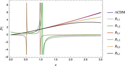
Dimensionless luminosity distance as function of the redshift for rational Chebyshev approximations of the second (R_{1, 1}), third (R_{1, 2}, R_{2, 1}), and fourth (R_{1, 3}, R_{2, 2}, R_{3, 1}) degrees, compared to the ΛCDM model. Here, divergences are due to the natural construction of rational approximations. Choosing arbitrarily the set of coefficients limits the possibility to plot in the whole domain the approximated cosmic distances. Choosing a viable set of priors over coefficients is the key to enable the correct orders of expansion in Chebyshev analyses.

Open in new tab Download slide

4.1 Calibrating Chebyshev polynomials with the concordance model

To check the accuracy of various Chebyshev approximations, we compare them with the Λ cold dark matter (ΛCDM) luminosity distance, |$d_{L}(z)\Big |_{\Lambda \text{CDM}}$|⁠:

\begin{eqnarray} d_{L}(z)\Big |_{\Lambda \text{CDM}}=(1+z)\int _{0}^{z}\frac{c\ \text{d}z^{\prime }}{H_{\Lambda \text{CDM}}(z^{\prime })}\,, \end{eqnarray}

(24)

in which we have

\begin{eqnarray} H_{\Lambda \text{CDM}}(z)= H_0\sqrt{\Omega _{m0}(1+z)^3+\Omega _{\Lambda }}\,. \end{eqnarray}

(25)

According to a spatially flat universe, we set Ω_Λ = 1 − Ω_m0, having Ω_m0 the matter density at current time. In the concordance paradigm case, the cosmographic parameters can be calculated in terms of Ω_m0:

\begin{eqnarray} q_{0, \Lambda \text{CDM}}&=& -1+\frac{3}{2}\Omega _{m0},\nonumber\\ j_{0, \Lambda \text{CDM}}&=&1,\nonumber\\ s_{0, \Lambda \text{CDM}}&=&1-\frac{9}{2}\Omega _{m0}. \end{eqnarray}

(26)

As an indicative possibility, we fix Ω_m0 = 0.3. So that from equation (26), one gets

\begin{eqnarray} \left\lbrace \begin{array}{c} q_0=-0.55\,, \\ j_0=1\,, \\ s_0=-0.35\,. \end{array} \right. \end{eqnarray}

(27)

Using the values of equation (27), in Fig. 1, we show the behaviour with the redshift of |$\overline{d_L}(z)\equiv \frac{H_0}{c}d_L(z)$| for different degrees of rational Chebyshev approximations.

In principle, to approximate the ΛCDM model some of the rational Chebyshev polynomials may present singularities turning out to give unsuitable outcomes. To overcome this issue, the preferred rational approximations are those with n − m ≥ 0, in analogy to what happens for Padé approximations (Aviles et al. 2014). In particular, as practically checked the approximant R_{2, 1}(z) seems to give the most accurate approximation to the luminosity distance of the ΛCDM model. Assuming that the calibration with the concordance paradigm would be viable for any possible dark energy term, we assume that the most suitable approximation with Chebyshev polynomials comes from R_{2, 1}(z).

To portray a qualitative representation of numerical improvements that one gains using our method, we compare R_{2, 1}(z) with the standard fourth-order Taylor expansion of d_L(z) given in equation (4), and with the (2,2) Padé approximation of d_L(z). We choose the (2,2) Padé approximation, since it has been argued that it is robustly characterized by good convergence properties (Aviles et al. 2014) as used in computational analyses. We note that, while in the Taylor and Padé approximations the snap parameter shows up at the fourth order, in the rational Chebyshev polynomials it is present from the lowest degrees, since all the coefficients c_k of equation (23) have been calculated from the Taylor series expansion of d_L(z) up to the snap order (as confirmed in equation 4). For comparison, we report the expression of the (2,2) Padé approximation of d_L(z) in Appendix B. In Fig. 2, we show the behaviour of |$\overline{d_L}(z)$| for the various techniques. As can be seen, the Taylor approach fails when z > 1. Our Chebyshev cosmography stands out for the excellent approximation to the ΛCDM luminosity distance, resulting mostly more effective than Padé approximations.

Figure 2.

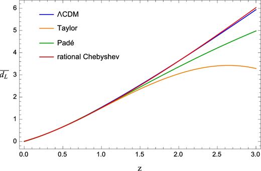
Dimensionless luminosity distance as function of the redshift for the ΛCDM model and its fourth-order Taylor, (2,2) Padé and (2,1) rational Chebyshev approximations. The maximum z for that the ΛCDM model is a good approximation is placed around z ∼ 3. This choice goes further than the highest redshift of BAO measurements and it turns out to be higher than supernova data.

Open in new tab Download slide

4.2 The convergence radius

We here argue how to broadcast the above considerations to well-motivated theoretical scenarios. Thus, we wonder whether Chebyshev cosmography is expected to effectively improve the approximations to cosmic distances than standard cosmography. To do so, it behooves us to check how much the aforementioned approximations are stable to higher redshifts. Hence, one can test the ability of the various cosmographic techniques, able to describe high-redshift domains, by a direct comparison amongst the corresponding convergence radii, here defined by ρ.

As a simple example, we explicitly calculate the convergence radius of the (1,1) rational Chebyshev approximation of the luminosity distance, compared to the second-order Taylor series and to the (1,1) Padé approximation. From equations (14) and (19), it holds

\begin{eqnarray} R_{1,1}(z)=\frac{a_0 T_0(z)+a_1T_1(z)}{1+b_1T_1(z)}=\frac{a_0+a_1 z}{1+b_1 z}\,, \end{eqnarray}

(28)

where the coefficients {a₀, a₁, b₁} are expressed in terms of the cosmographic series as shown in equation (A1). We can rearrange equation (28) as

\begin{eqnarray} R_{1,1}=\frac{a_0}{1+b_1 z}+\frac{a_1}{b_1}\left(1-\frac{1}{1+b_1 z}\right), \end{eqnarray}

(29)

and, after some algebra, one obtains

\begin{eqnarray} R_{1,1}=\frac{a_1}{b_1}+\left(a_0-\frac{a_1}{b_1}\right)\sum _{n=0}^{\infty }(-b_1)^n z^n\,. \end{eqnarray}

(30)

The geometric series in equation (30) converges for |z| < 1/|b₁|, so that the convergence radius of the (1,1) rational Chebyshev approximation of d_L(z) is

\begin{eqnarray} \rho _{R_{1,1}}&=&\frac{1}{|b_1|} \nonumber \\ &=&\bigg |\frac{-3 (7 - j_0 + q_0 + 3 q_0^2)}{14 + 5 j_0 (1 + 2 q_0) - q_0 \big (14 + 15 q_0 (1 + q_0)\big ) + s_0}\bigg |. \end{eqnarray}

(31)

Analogous calculations show that the convergence radius of the (1,1) Padé approximant for d_L(z) is

\begin{eqnarray} \rho _{P_{1,1}}=\frac{2}{1-q_0}\,. \end{eqnarray}

(32)

The convergence radius of the second-order Taylor series of d_L(z) is approximately given by

\begin{eqnarray} \rho _{d_{L,2}}=\frac{1-q_0}{2}\,. \end{eqnarray}

(33)

For the sake of completeness, the numerical values of |$\rho _{R_{1,1}}, \rho _{P_{1,1}}$|⁠, and |$\rho _{d_{L,2}}$| should be computed by using fitting results over the cosmographic coefficients. However, an analogous check can be made assuming the reference values equation (26). In such a case, one gets

\begin{eqnarray} \left\lbrace \begin{array}{c} \rho _{R_{1,1}}=1.014\,, \\ \rho _{P_{1,1}}= 1.290\,, \\ \rho _{d_{L,2}}=0.775\,. \end{array} \right. \end{eqnarray}

(34)

These indicative results confirm the improvements of the rational polynomials in extending the radius of convergence with respect to the Taylor series. From the outcomes of equation (26), we notice that the convergence radius of the Padé approximation seems fairly better than the Chebyshev one. However, this is due to the choice made on the set q₀, j₀, and s₀. In Fig. 3, we plot the convergence radii for Taylor, Padé, and Chebyshev polynomials with a different set of cosmographic coefficients not calibrated over the concordance paradigm. In Fig. 3, in particular, we show the regions in which the improvements of Chebyshev rational approximations become significant in terms of the convergence radius.

Figure 3.

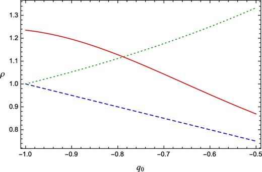
Convergence radii for the second-order Taylor (dashed curve), (1,1) Padé (dotted curve), and (1,1) rational Chebyshev (solid curve) approximations of the luminosity distance as a function of q₀. For the rational Chebyshev approximation, we used the indicative values of j₀ = 2, s₀ = −1.

Open in new tab Download slide

5 OBSERVATIONAL CONSTRAINTS

In this section, we present the data we use to set bounds on the cosmographic parameters.

5.1 Supernovae Ia

In this work, we test the JLA sample of 740 SNe of type Ia (Betoule et al. 2014) in the redshift interval 0.01 < z < 1.3. All the SNe have been standardized using the SALT2 model (Guy et al. 2007) as fitter for their light curves. The catalogue provides, for each SN, the redshift z, model-independent apparent magnitude in the B band (m_B), the stretch factor of the light curve (X₁), and the colour at maximum brightness (C). The theoretical distance modulus,

\begin{eqnarray} \mu _{\text{th}}(z)=25+5\log _{10}[d_L(z)]\,, \end{eqnarray}

(35)

is parametrized as follows:

\begin{eqnarray} \mu _{\text{obs}}=m_B-(M_B-\alpha X_1+\beta C)\,, \end{eqnarray}

(36)

where the absolute magnitude is defined as

\begin{eqnarray} M_B= \left\lbrace \begin{array}{@{}l@{\quad }l@{}}M, & \text{if}\ M_{\text{host}}<10^{10}M_{\text{Sun}}\\ M+\Delta _M, & \text{otherwise} \end{array}\right. \end{eqnarray}

(37)

being M_host the host stellar mass. The nuisance parameters {M, Δ_M, α, β} are fitted together with the cosmological parameters. The normalized likelihood function of the SNe data is given by

\begin{eqnarray} \mathcal {L}_{SN}=\frac{1}{{|2\pi {\bf C}|}^{1/2}}\exp \left[-\frac{1}{2}\left(\mu _{\text{th}}-\mu _{\text{obs}}\right)^\dagger {\bf C}^{-1}\left(\mu _{\text{th}}-\mu _{\text{obs}}\right)\right], \end{eqnarray}

(38)

where C is the 2220 × 2200 covariance matrix constructed as in Betoule et al. (2014), which includes statistical and systematic uncertainties on the light-curve parameters.

5.2 Observational Hubble data

The Hubble rate of a given cosmological model can be constrained by means of the model-independent measurements acquired through the differential age (DA) method, first presented in Jimenez & Loeb (2002). Such a technique uses red passively evolving galaxies as cosmic chronometers. In particular, one can obtain H(z) by measuring the age difference of two close galaxies and using the relation

\begin{eqnarray} H_{\text{th}}(z)=-\frac{1}{(1+z)}{\left(\frac{{\rm d}t}{{\rm d}z}\right)}^{-1}\,. \end{eqnarray}

(39)

The normalized likelihood function for the OHD data |$(\mathcal {L}_{\text{OHD}})$| is built using a collection of 31 uncorrelated DA measurements of H(z), which we report in Appendix C:

\begin{eqnarray} \mathcal {L}_{\text{OHD}}=\frac{\exp \left[-\frac{1}{2}\displaystyle {\sum _{i=1}^{31}}\left(\frac{H_{\text{th}}(z_i)-H_{\text{obs}}(z_i)}{\sigma _{H,i}}\right)^2\right]}{\left[{(2\pi )}^{31}\displaystyle {\prod _{i=1}^{31}} \sigma _{H,i}^2\right]^{1/2}}\,. \end{eqnarray}

(40)

5.3 Baryon acoustic oscillations

Intensive studies on the large-scale structures of the universe have been done thanks to galaxy surveys. The baryon acoustic oscillations that occur in the relativistic plasma come in the form of a characteristic peak in the galaxy correlation function. The BAO measurements are usually given in the literature as |$d_V^{\text{th}}(z)\equiv r_d/D_V(z)$|⁠, namely the ratio between the comoving sound horizon at the drag epoch (r_d) and the spherically averaged distance measure introduced in Eisenstein et al. (2005):

\begin{eqnarray} D_V(z)= \left[\frac{{d_L}^2(z)}{(1+z)^2}\frac{c\ z}{H(z)}\right]^{1/3}. \end{eqnarray}

(41)

We construct the normalized likelihood function for the BAO data using the six uncorrelated and model-independent measurements given in Lukovic, D'Agostino & Vittorio (2016), which we list in Appendix C:

\begin{eqnarray} \mathcal {L}_{\text{BAO}}=\frac{\exp {\left[-\frac{1}{2}\displaystyle {\sum _{i=1}^6}\left(\frac{d_V^{\text{th}}(z_i)-d_V^{\text{obs}}(z_i)}{\sigma _{d_{V,i}}}\right)^2\right]}}{\left[{(2\pi )}^6\displaystyle {\prod _{i=1}^6}\sigma _{d_{V,i}}^2\right]^{1/2}}\,. \end{eqnarray}

(42)

5.4 Results of the Monte Carlo analysis

To test the different cosmographic approaches, we performed a Markov Chain Monte Carlo (MCMC) integration on the combined likelihood of the data sets we presented above:

\begin{eqnarray} \mathcal {L}_{\text{joint}}=\mathcal {L}_{\text{SN}}\times \mathcal {L}_{\text{OHD}}\times \mathcal {L}_{\text{BAO}}\,. \end{eqnarray}

(43)

We implemented the Metropolis–Hastings algorithm with the Monte python code (Audren et al. 2013), assuming uniform priors for the parameters (see Table 1). The numerical results of our joint analysis are shown in Table 2. Also, in Figs 4– 6, we show the marginalized 2D 1σ and 2σ regions and the 1D posterior distributions for the cosmological and nuisance parameters in the case of the three cosmographic techniques. Our results prove that the method of rational Chebyshev polynomials reduces the uncertainties in the estimate of the cosmographic parameters with respect to the other approaches, as shown by the relative errors in Table 3.

Figure 4.

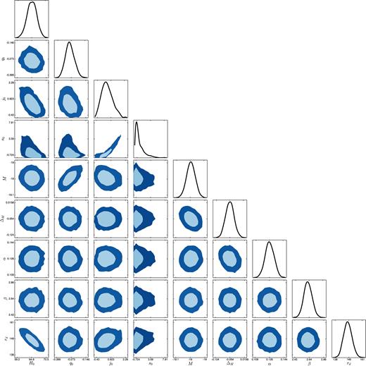
68 per cent and 95 per cent confidence level contours and posterior distributions from the MCMC analysis of SN+OHD+BAO data for the fourth-order Taylor approximation of the luminosity distance. H₀ is expressed in km s⁻¹ Mpc⁻¹, and r_d in Mpc.

Open in new tab Download slide

Figure 5.

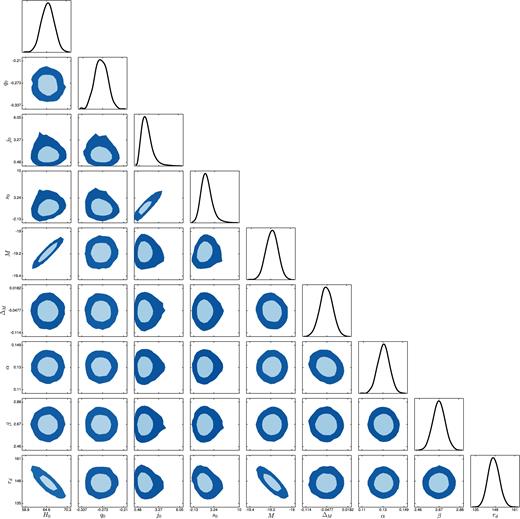
68 per cent and 95 per cent confidence level contours and posterior distributions from the MCMC analysis of SN+OHD+BAO data for the (2,2) Padé approximation of the luminosity distance. H₀ is expressed in km s⁻¹ Mpc⁻¹, and r_d in Mpc.

Open in new tab Download slide

Figure 6.

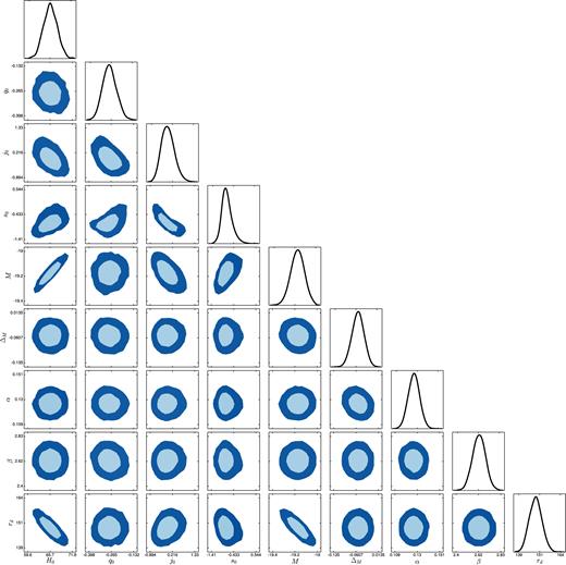
68 per cent and 95 per cent confidence level contours and posterior distributions from the MCMC analysis of SN+OHD+BAO data for the (2,1) rational Chebyshev approximation of the luminosity distance. H₀ is expressed in km s⁻¹ Mpc⁻¹, and r_d in Mpc.

Open in new tab Download slide

Table 1.

Open in new tab

Priors for parameters estimate in the MCMC numerical analysis. H₀ values are given in units of km s⁻¹ Mpc⁻¹, while r_d values in units of Mpc.

Parameters	Priors
H₀	(50, 90)
q₀	(−10, 10)
j₀	(−10, 10)
s₀	(−10, 10)
M	(−20, −18)
Δ_M	(−1, 1)
α	(0, 1)
β	(0, 5)
r_d	(140, 160)

Table 1.

Open in new tab

Priors for parameters estimate in the MCMC numerical analysis. H₀ values are given in units of km s⁻¹ Mpc⁻¹, while r_d values in units of Mpc.

Parameters	Priors
H₀	(50, 90)
q₀	(−10, 10)
j₀	(−10, 10)
s₀	(−10, 10)
M	(−20, −18)
Δ_M	(−1, 1)
α	(0, 1)
β	(0, 5)
r_d	(140, 160)

Table 2.

Open in new tab

68 per cent and 95 per cent confidence level parameter constraints from the MCMC analysis of SN+OHD+BAO data for the fourth-order Taylor, (2,2) Padé and (2,1) rational Chebyshev polynomial approximations of the luminosity distance. H₀ values are given in units of km s⁻¹ Mpc⁻¹, while r_d values in units of Mpc.

Parameter	Taylor			Padé			Rational Chebyshev
	Mean	1σ	2σ	Mean	1σ	2σ	Mean	1σ	2σ
H₀	65.80	\|$^{+2.09}_{-2.11}$\|	\|$^{+4.22}_{-4.00}$\|	64.94	\|$^{+2.11}_{-2.02}$\|	\|$^{+4.12}_{-4.13}$\|	64.95	\|$^{+1.89}_{-1.94}$\|	\|$^{+3.77}_{-3.77}$\|
q₀	−0.276	\|$^{+0.043}_{-0.049}$\|	\|$^{+0.093}_{-0.091}$\|	−0.285	\|$^{+0.040}_{-0.046}$\|	\|$^{+0.087}_{-0.084}$\|	−0.278	\|$^{+0.021}_{-0.021}$\|	\|$^{+0.041}_{-0.042}$\|
j₀	−0.023	\|$^{+0.317}_{-0.397}$\|	\|$^{+0.748}_{-0.685}$\|	0.545	\|$^{+0.463}_{-0.652}$\|	\|$^{+1.135}_{-1.025}$\|	1.585	\|$^{+0.497}_{-0.914}$\|	\|$^{+1.594}_{-1.453}$\|
s₀	−0.745	\|$^{+0.196}_{-0.284}$\|	\|$^{+0.564}_{-0.487}$\|	0.118	\|$^{+0.451}_{-1.600}$\|	\|$^{+3.422}_{-1.921}$\|	1.041	\|$^{+1.183}_{-1.784}$\|	\|$^{+3.388}_{-3.087}$\|
M	−19.16	\|$^{+0.07}_{-0.07}$\|	\|$^{+0.14}_{-0.14}$\|	−19.03	\|$^{+0.02}_{-0.02}$\|	\|$^{+0.05}_{-0.05}$\|	−19.17	\|$^{+0.07}_{-0.07}$\|	\|$^{+0.13}_{-0.13}$\|
Δ_M	−0.054	\|$^{+0.023}_{-0.022}$\|	\|$^{+0.044}_{-0.045}$\|	−0.054	\|$^{+0.022}_{-0.023}$\|	\|$^{+0.045}_{-0.045}$\|	−0.050	\|$^{+0.022}_{-0.022}$\|	\|$^{+0.044}_{-0.045}$\|
α	0.127	\|$^{+0.006}_{-0.006}$\|	\|$^{+0.012}_{-0.012}$\|	0.127	\|$^{+0.006}_{-0.006}$\|	\|$^{+0.012}_{-0.012}$\|	0.130	\|$^{+0.006}_{-0.006}$\|	\|$^{+0.012}_{-0.012}$\|
β	2.624	\|$^{+0.071}_{-0.068}$\|	\|$^{+0.136}_{-0.140}$\|	2.625	\|$^{+0.065}_{-0.069}$\|	\|$^{+0.137}_{-0.135}$\|	2.667	\|$^{+0.068}_{-0.069}$\|	\|$^{+0.137}_{-0.135}$\|
r_d	149.2	\|$^{+3.7}_{-4.1}$\|	\|$^{+7.7}_{-7.5}$\|	148.6	\|$^{+3.5}_{-3.8}$\|	\|$^{+7.5}_{-7.1}$\|	147.2	\|$^{+3.7}_{-4.0}$\|	\|$^{+7.8}_{-7.5}$\|

Parameter	Taylor			Padé			Rational Chebyshev
	Mean	1σ	2σ	Mean	1σ	2σ	Mean	1σ	2σ
H₀	65.80	\|$^{+2.09}_{-2.11}$\|	\|$^{+4.22}_{-4.00}$\|	64.94	\|$^{+2.11}_{-2.02}$\|	\|$^{+4.12}_{-4.13}$\|	64.95	\|$^{+1.89}_{-1.94}$\|	\|$^{+3.77}_{-3.77}$\|
q₀	−0.276	\|$^{+0.043}_{-0.049}$\|	\|$^{+0.093}_{-0.091}$\|	−0.285	\|$^{+0.040}_{-0.046}$\|	\|$^{+0.087}_{-0.084}$\|	−0.278	\|$^{+0.021}_{-0.021}$\|	\|$^{+0.041}_{-0.042}$\|
j₀	−0.023	\|$^{+0.317}_{-0.397}$\|	\|$^{+0.748}_{-0.685}$\|	0.545	\|$^{+0.463}_{-0.652}$\|	\|$^{+1.135}_{-1.025}$\|	1.585	\|$^{+0.497}_{-0.914}$\|	\|$^{+1.594}_{-1.453}$\|
s₀	−0.745	\|$^{+0.196}_{-0.284}$\|	\|$^{+0.564}_{-0.487}$\|	0.118	\|$^{+0.451}_{-1.600}$\|	\|$^{+3.422}_{-1.921}$\|	1.041	\|$^{+1.183}_{-1.784}$\|	\|$^{+3.388}_{-3.087}$\|
M	−19.16	\|$^{+0.07}_{-0.07}$\|	\|$^{+0.14}_{-0.14}$\|	−19.03	\|$^{+0.02}_{-0.02}$\|	\|$^{+0.05}_{-0.05}$\|	−19.17	\|$^{+0.07}_{-0.07}$\|	\|$^{+0.13}_{-0.13}$\|
Δ_M	−0.054	\|$^{+0.023}_{-0.022}$\|	\|$^{+0.044}_{-0.045}$\|	−0.054	\|$^{+0.022}_{-0.023}$\|	\|$^{+0.045}_{-0.045}$\|	−0.050	\|$^{+0.022}_{-0.022}$\|	\|$^{+0.044}_{-0.045}$\|
α	0.127	\|$^{+0.006}_{-0.006}$\|	\|$^{+0.012}_{-0.012}$\|	0.127	\|$^{+0.006}_{-0.006}$\|	\|$^{+0.012}_{-0.012}$\|	0.130	\|$^{+0.006}_{-0.006}$\|	\|$^{+0.012}_{-0.012}$\|
β	2.624	\|$^{+0.071}_{-0.068}$\|	\|$^{+0.136}_{-0.140}$\|	2.625	\|$^{+0.065}_{-0.069}$\|	\|$^{+0.137}_{-0.135}$\|	2.667	\|$^{+0.068}_{-0.069}$\|	\|$^{+0.137}_{-0.135}$\|
r_d	149.2	\|$^{+3.7}_{-4.1}$\|	\|$^{+7.7}_{-7.5}$\|	148.6	\|$^{+3.5}_{-3.8}$\|	\|$^{+7.5}_{-7.1}$\|	147.2	\|$^{+3.7}_{-4.0}$\|	\|$^{+7.8}_{-7.5}$\|

Table 2.

Open in new tab

68 per cent and 95 per cent confidence level parameter constraints from the MCMC analysis of SN+OHD+BAO data for the fourth-order Taylor, (2,2) Padé and (2,1) rational Chebyshev polynomial approximations of the luminosity distance. H₀ values are given in units of km s⁻¹ Mpc⁻¹, while r_d values in units of Mpc.

Parameter	Taylor			Padé			Rational Chebyshev
	Mean	1σ	2σ	Mean	1σ	2σ	Mean	1σ	2σ
H₀	65.80	\|$^{+2.09}_{-2.11}$\|	\|$^{+4.22}_{-4.00}$\|	64.94	\|$^{+2.11}_{-2.02}$\|	\|$^{+4.12}_{-4.13}$\|	64.95	\|$^{+1.89}_{-1.94}$\|	\|$^{+3.77}_{-3.77}$\|
q₀	−0.276	\|$^{+0.043}_{-0.049}$\|	\|$^{+0.093}_{-0.091}$\|	−0.285	\|$^{+0.040}_{-0.046}$\|	\|$^{+0.087}_{-0.084}$\|	−0.278	\|$^{+0.021}_{-0.021}$\|	\|$^{+0.041}_{-0.042}$\|
j₀	−0.023	\|$^{+0.317}_{-0.397}$\|	\|$^{+0.748}_{-0.685}$\|	0.545	\|$^{+0.463}_{-0.652}$\|	\|$^{+1.135}_{-1.025}$\|	1.585	\|$^{+0.497}_{-0.914}$\|	\|$^{+1.594}_{-1.453}$\|
s₀	−0.745	\|$^{+0.196}_{-0.284}$\|	\|$^{+0.564}_{-0.487}$\|	0.118	\|$^{+0.451}_{-1.600}$\|	\|$^{+3.422}_{-1.921}$\|	1.041	\|$^{+1.183}_{-1.784}$\|	\|$^{+3.388}_{-3.087}$\|
M	−19.16	\|$^{+0.07}_{-0.07}$\|	\|$^{+0.14}_{-0.14}$\|	−19.03	\|$^{+0.02}_{-0.02}$\|	\|$^{+0.05}_{-0.05}$\|	−19.17	\|$^{+0.07}_{-0.07}$\|	\|$^{+0.13}_{-0.13}$\|
Δ_M	−0.054	\|$^{+0.023}_{-0.022}$\|	\|$^{+0.044}_{-0.045}$\|	−0.054	\|$^{+0.022}_{-0.023}$\|	\|$^{+0.045}_{-0.045}$\|	−0.050	\|$^{+0.022}_{-0.022}$\|	\|$^{+0.044}_{-0.045}$\|
α	0.127	\|$^{+0.006}_{-0.006}$\|	\|$^{+0.012}_{-0.012}$\|	0.127	\|$^{+0.006}_{-0.006}$\|	\|$^{+0.012}_{-0.012}$\|	0.130	\|$^{+0.006}_{-0.006}$\|	\|$^{+0.012}_{-0.012}$\|
β	2.624	\|$^{+0.071}_{-0.068}$\|	\|$^{+0.136}_{-0.140}$\|	2.625	\|$^{+0.065}_{-0.069}$\|	\|$^{+0.137}_{-0.135}$\|	2.667	\|$^{+0.068}_{-0.069}$\|	\|$^{+0.137}_{-0.135}$\|
r_d	149.2	\|$^{+3.7}_{-4.1}$\|	\|$^{+7.7}_{-7.5}$\|	148.6	\|$^{+3.5}_{-3.8}$\|	\|$^{+7.5}_{-7.1}$\|	147.2	\|$^{+3.7}_{-4.0}$\|	\|$^{+7.8}_{-7.5}$\|

Parameter	Taylor			Padé			Rational Chebyshev
	Mean	1σ	2σ	Mean	1σ	2σ	Mean	1σ	2σ
H₀	65.80	\|$^{+2.09}_{-2.11}$\|	\|$^{+4.22}_{-4.00}$\|	64.94	\|$^{+2.11}_{-2.02}$\|	\|$^{+4.12}_{-4.13}$\|	64.95	\|$^{+1.89}_{-1.94}$\|	\|$^{+3.77}_{-3.77}$\|
q₀	−0.276	\|$^{+0.043}_{-0.049}$\|	\|$^{+0.093}_{-0.091}$\|	−0.285	\|$^{+0.040}_{-0.046}$\|	\|$^{+0.087}_{-0.084}$\|	−0.278	\|$^{+0.021}_{-0.021}$\|	\|$^{+0.041}_{-0.042}$\|
j₀	−0.023	\|$^{+0.317}_{-0.397}$\|	\|$^{+0.748}_{-0.685}$\|	0.545	\|$^{+0.463}_{-0.652}$\|	\|$^{+1.135}_{-1.025}$\|	1.585	\|$^{+0.497}_{-0.914}$\|	\|$^{+1.594}_{-1.453}$\|
s₀	−0.745	\|$^{+0.196}_{-0.284}$\|	\|$^{+0.564}_{-0.487}$\|	0.118	\|$^{+0.451}_{-1.600}$\|	\|$^{+3.422}_{-1.921}$\|	1.041	\|$^{+1.183}_{-1.784}$\|	\|$^{+3.388}_{-3.087}$\|
M	−19.16	\|$^{+0.07}_{-0.07}$\|	\|$^{+0.14}_{-0.14}$\|	−19.03	\|$^{+0.02}_{-0.02}$\|	\|$^{+0.05}_{-0.05}$\|	−19.17	\|$^{+0.07}_{-0.07}$\|	\|$^{+0.13}_{-0.13}$\|
Δ_M	−0.054	\|$^{+0.023}_{-0.022}$\|	\|$^{+0.044}_{-0.045}$\|	−0.054	\|$^{+0.022}_{-0.023}$\|	\|$^{+0.045}_{-0.045}$\|	−0.050	\|$^{+0.022}_{-0.022}$\|	\|$^{+0.044}_{-0.045}$\|
α	0.127	\|$^{+0.006}_{-0.006}$\|	\|$^{+0.012}_{-0.012}$\|	0.127	\|$^{+0.006}_{-0.006}$\|	\|$^{+0.012}_{-0.012}$\|	0.130	\|$^{+0.006}_{-0.006}$\|	\|$^{+0.012}_{-0.012}$\|
β	2.624	\|$^{+0.071}_{-0.068}$\|	\|$^{+0.136}_{-0.140}$\|	2.625	\|$^{+0.065}_{-0.069}$\|	\|$^{+0.137}_{-0.135}$\|	2.667	\|$^{+0.068}_{-0.069}$\|	\|$^{+0.137}_{-0.135}$\|
r_d	149.2	\|$^{+3.7}_{-4.1}$\|	\|$^{+7.7}_{-7.5}$\|	148.6	\|$^{+3.5}_{-3.8}$\|	\|$^{+7.5}_{-7.1}$\|	147.2	\|$^{+3.7}_{-4.0}$\|	\|$^{+7.8}_{-7.5}$\|

Table 3.

Open in new tab

68 per cent and 95 per cent relative uncertainties on the estimate of the cosmographic parameters from the MCMC analysis of SN+OHD+BAO data for the fourth-order Taylor, (2,2) Padé and (2,1) rational Chebyshev polynomial approximations of the luminosity distance.

Parameter	Taylor		Padé		Rational Chebyshev
	1σ( per cent)	2σ( per cent)	\|$1\sigma\,\,(\rm{per\,\,cent})$\|	\|$2\sigma\,\,(\rm{per\,\,cent})$\|	\|$1\sigma\,\,(\rm{per\,\,cent})$\|	\|$2\sigma\,\,(\rm{per\,\,cent})$\|
H₀	3.19	6.25	3.17	6.35	2.95	4.11
q₀	16.8	33.5	15.1	30.1	7.66	14.8
j₀	1534	3079	102	198	44.5	96.1
s₀	32.2	70.5	866	2258	142	311

Parameter	Taylor		Padé		Rational Chebyshev
	1σ( per cent)	2σ( per cent)	\|$1\sigma\,\,(\rm{per\,\,cent})$\|	\|$2\sigma\,\,(\rm{per\,\,cent})$\|	\|$1\sigma\,\,(\rm{per\,\,cent})$\|	\|$2\sigma\,\,(\rm{per\,\,cent})$\|
H₀	3.19	6.25	3.17	6.35	2.95	4.11
q₀	16.8	33.5	15.1	30.1	7.66	14.8
j₀	1534	3079	102	198	44.5	96.1
s₀	32.2	70.5	866	2258	142	311

Table 3.

Open in new tab

68 per cent and 95 per cent relative uncertainties on the estimate of the cosmographic parameters from the MCMC analysis of SN+OHD+BAO data for the fourth-order Taylor, (2,2) Padé and (2,1) rational Chebyshev polynomial approximations of the luminosity distance.

Parameter	Taylor		Padé		Rational Chebyshev
	1σ( per cent)	2σ( per cent)	\|$1\sigma\,\,(\rm{per\,\,cent})$\|	\|$2\sigma\,\,(\rm{per\,\,cent})$\|	\|$1\sigma\,\,(\rm{per\,\,cent})$\|	\|$2\sigma\,\,(\rm{per\,\,cent})$\|
H₀	3.19	6.25	3.17	6.35	2.95	4.11
q₀	16.8	33.5	15.1	30.1	7.66	14.8
j₀	1534	3079	102	198	44.5	96.1
s₀	32.2	70.5	866	2258	142	311

Parameter	Taylor		Padé		Rational Chebyshev
	1σ( per cent)	2σ( per cent)	\|$1\sigma\,\,(\rm{per\,\,cent})$\|	\|$2\sigma\,\,(\rm{per\,\,cent})$\|	\|$1\sigma\,\,(\rm{per\,\,cent})$\|	\|$2\sigma\,\,(\rm{per\,\,cent})$\|
H₀	3.19	6.25	3.17	6.35	2.95	4.11
q₀	16.8	33.5	15.1	30.1	7.66	14.8
j₀	1534	3079	102	198	44.5	96.1
s₀	32.2	70.5	866	2258	142	311

An alternative approach is to start from the cosmographic expansion series of the Hubble rate and, then, evaluate the luminosity distance by numerical integrations, as pointed out in Aviles, Klapp & Luongo (2017). However, it turns out that the analysis based on rational Chebyshev approximations of H(z) does not lead to further reduction of the error propagation with respect to our original approach. An interesting fact is that, by construction, one uses Chebyshev polynomials with lower orders than Taylor series and Padé approximants. This mostly reduces the computational difficulties in implementing cosmic data, although does not accurately fixes the highest-order parameter in the approximation. This is the case of s₀ whose error bars are not significatively improved adopting Chebyshev polynomials. To overcome this issue, it would be enough to increase the Chebyshev order to better fix s₀ than Taylor and Padé treatments.

6 SUMMARY AND CONCLUSIONS

In this work, we revised the convergence problem in cosmography, adopting a new method to reduce error uncertainties and bias propagations as high-redshift data are used. We set bounds on the cosmographic series, considering rational approximations of the luminosity distance and we demonstrated that such approximations are also valid for any cosmic distances. In particular, our novel procedure is based on approximating the luminosity distance d_L(z) with ratios of Chebyshev polynomials. Since, by definition, Chebyshev approximants are the most suitable polynomials in approximating functions, we expected to get fairly good outcomes in computing cosmographic series. Indeed, we found that our approach overcomes the convergence issues typical of standard cosmographic techniques based on Taylor approximations. This has been confirmed by computing convergence radii for different sets of cosmographic coefficients. We also compared our new approach with the consolidate procedure of Padé expansions. We showed that both numerical bounds and convergence radii are improved under precise conditions. This naturally showed that Chebyshev rational polynomials are more suitable to describe the cosmic dynamics at z > 1 than Padé series. Bearing this in mind, through the predictions of the concordance ΛCDM model, we calibrated the orders of Chebyshev rational polynomials, providing the recipe of a new Chebyshev cosmography, which turned out to be more predictive than Taylor series at all redshift domains. We evaluated the (2,1) Chebyshev series, corresponding to a fourth-order Tayor series and to a (2,2) Padé approximation. This showed that lower order Chebyshev series work better than higher ones constructed by Taylor and Padé recipes. We finally checked the goodness of our method, statistically combining the JLA supernova compilation, H(z) differential age data, and baryon acoustic oscillation measurements by performing Monte Carlo integrations based on the Metropolis–Hastings algorithm. To do so, we employed the free available Monte python code and we computed the corresponding contours up to the |$95\,\,\rm{per\,\,cent}$| confidence level. The numerical improvements have been reported in terms of percentages on 1σ and 2σ confidence levels. The error percentages are severely lowered, whereas the mean values are centred around intervals compatible with previous results on cosmography.

Our final outcomes forecast that the technique of Chebyshev cosmography substantially decreases the relative uncertainties on the estimates of cosmographic parameters respect to other previous approaches. This procedure candidates as a new way towards computing the cosmographic series and to better fix constraints on cosmography. Chebyshev cosmography is thus able to heal previous inconsistencies on convergence that plagued cosmography itself. Further, it enables to use high-redshift data surveys in cosmographic analyses with no large spreads overfitted coefficients.

Future efforts will be devoted to match Padé and Chebyshev techniques in different redshift domains. We will work on characterizing the cosmographic data over binning intervals in which one will be able to highly maximize both the convergence radii and mean values and to minimize both bias and uncertainties on free cosmographic coefficients. Hence, it will be possible to go further with our approximation, even investigating Chebyshev approximations using future data got for example from the cosmic microwave domain.

ACKNOWLEDGEMENTS

This paper is based upon work from COST action CA15117 (CANTATA), supported by COST (European Cooperation in Science and Technology). The authors warmly thank the anonymous referee for comments and suggestions that permitted to improve the quality of the paper. S.C. acknowledges the support of INFN (iniziativa specifica QGSKY). R.D. thanks Federico Tosone for useful discussions on the Monte python code.

Footnotes

1

The assumption of flatness overcomes problems of degeneracy amongst the cosmographic parameters entering the expression of the luminosity distance (Dunsby & Luongo 2016).

2

In principle, one may go further in the expansion and consider higher order coefficients. We limit our study up to the snap, since the next cosmographic parameters are poorly constrained by observations (Aviles et al. 2012).

3

Throughout the text, we refer to the Chebyshev polynomials of the first kind simply as Chebyshev polynomials.

4

We here truncate our analysis to the fifth order, since additional contributions go beyond our treatment. In so doing, we arrive to analyse up to snap parameter s₀.

REFERENCES

Anderson

L.

et al. ,

2014

,

MNRAS

,

441

,

24

Crossref

Search ADS

Arabsalmani

M.

,

Sahni

V.

,

2011

,

Phys. Rev. D

,

83

,

04350

Crossref

Search ADS

Audren

B.

,

Lesgourgues

J.

,

Benabed

K.

,

Prunet

S.

,

2013

,

J. Cosmol. Astropart. Phys.

,

02

,

001

Crossref

Search ADS

Aviles

A.

,

Gruber

C.

,

Luongo

O.

,

Quevedo

H.

,

2012

,

Phys. Rev. D

,

86

,

123516

Crossref

Search ADS

Aviles

A.

,

Bravetti

A.

,

Capozziello

S.

,

Luongo

O.

,

2014

,

Phys. Rev. D

,

90

,

043531

Crossref

Search ADS

Aviles

A.

,

Klapp

J.

,

Luongo

O.

,

2017

,

Phys. Dark Univ.

,

17

,

25

Crossref

Search ADS

Baker

G. A.

Jr,

Graves-Morris

P.

,

1996

,

Padé Approximants

.

Cambridge Univ. Press

Bamba

K.

,

Capozziello

S.

,

Nojiri

S.

,

Odintsov

S. D.

,

2012

,

Astroph. and Sp. Sci.

342

,

155

Crossref

Search ADS

Betoule

M.

et al. ,

2014

,

A&A

,

568

,

A22

Crossref

Search ADS

Beutler

F.

et al. ,

2011

,

MNRAS

,

416

,

3017

Crossref

Search ADS

Busti

V. C.

,

de la

Cruz-Dombriz A.

,

Dunsby

P. K. S.

,

Sez-Gmez

D.

,

2015

,

Phys. Rev. D

,

92

,

123512

Crossref

Search ADS

Cai

R.

,

Tuo

Z.

,

2011

,

Phys. Lett. B

,

706

,

116

Crossref

Search ADS

Capozziello

S.

,

Lazkoz

R.

,

Salzano

V.

,

2011

,

Phys. Rev. D

,

84

,

124061

Crossref

Search ADS

Capozziello

S.

,

Farooq

O.

,

Luongo

O.

,

Ratra

B.

,

2014

,

Phys. Rev. D

,

90

,

044016

Crossref

Search ADS

Capozziello

S.

,

Luongo

O.

,

Saridakis

E. N.

,

2015

,

Phys. Rev. D

,

91

,

124037

Crossref

Search ADS

Carvalho

J. C.

,

Alcaniz

J. S.

,

2011

,

MNRAS

,

418

,

1873

Crossref

Search ADS

Cattoën

C.

,

Visser

M.

,

2007

,

Class. Quant. Grav.

,

24

,

5985

Crossref

Search ADS

Cattoën

C.

,

Visser

M.

,

2008

,

Phys. Rev. D

,

78

,

063501

Crossref

Search ADS

Chebyshev

P. L.

,

1854

,

Mémoires des Savants étrangers présentés á l'Académie de Saint-Pétersbourg

,

7

,

539

Chuang

C. H.

,

Wang

Y.

,

2012

,

MNRAS

,

426

,

226

Crossref

Search ADS

Delubac

T.

et al. ,

2015

,

A&A

,

574

,

A59

Crossref

Search ADS

Demianski

M.

,

Piedipalumbo

E.

,

Rubano

C.

,

Scudellaro

P.

,

2012

,

MNRAS

,

426

,

1396

Crossref

Search ADS

Demianski

M.

,

Piedipalumbo

E.

,

Sawant

D.

,

Amati

L.

,

2017

,

A&A

,

598

,

A113

Crossref

Search ADS

Dunsby

P. K. S.

,

Luongo

O.

,

2016

,

Int. J. Geom. Meth. Mod. Phys.

,

13

,

1630002

Crossref

Search ADS

Eisenstein

D. J.

et al. ,

2005

,

AJ

,

633

,

560

Crossref

Search ADS

Font-Ribera

A.

et al. ,

2014

,

J. Cosmol. Astropart. Phys.

,

5

,

27

Crossref

Search ADS

Gerald

C. F.

,

Wheatley

P. O.

,

2003

,

Applied Numerical Analysis

.

Prentice Hall College Div

,

NJ

Google Scholar

Google Preview

OpenURL Placeholder Text

WorldCat

Gruber

C.

,

Luongo

O.

,

2014

,

Phys. Rev. D

,

89

,

103506

Crossref

Search ADS

Guimaraes

A. C. C.

,

Lima

J. A. S.

,

2011

,

Class. Quant. Grav.

,

28

,

125026

Crossref

Search ADS

Guy

J.

et al. ,

2007

,

A&A

,

466

,

11

Crossref

Search ADS

Harrison

E. R.

,

1976

,

Nature

,

260

,

591

Crossref

Search ADS

Jimenez

R.

,

Loeb

A.

,

2002

,

AJ

,

573

,

37

Crossref

Search ADS

Litvinov

G.

,

1993

,

Appl. Russ. J. Math. Phys.

,

1

,

313

Lukovic

V.

,

D'Agostino

R.

,

Vittorio

N.

,

2016

,

A&A

,

595

,

A109

Crossref

Search ADS

Luongo

O.

,

2011

,

Mod. Phys. Lett. A

,

26

,

1459

Crossref

Search ADS

Moresco

M.

,

2015

,

MNRAS

,

450

,

L16

Crossref

Search ADS

Moresco

M.

et al. ,

2012

,

J. Cosmol. Astropart. Phys.

,

8

,

006

Crossref

Search ADS

Moresco

M.

et al. ,

2016

,

J. Cosmol. Astropart. Phys.

,

05

,

014

Crossref

Search ADS

Perlmutter

S.

et al. ,

1999

,

ApJ

,

517

,

565

Crossref

Search ADS

Piedipalumbo

E.

,

Della Moglie

E.

,

Cianci

R.

,

2015

,

Int. J. Mod. Phys. D

,

24

,

1550100

Crossref

Search ADS

Planck Collaboration XIII

,

2016

,

A&A

,

594

,

A13

Crossref

Search ADS

Poplawski

N.

,

2006

,

Phys. Lett. B

,

640

,

135

Crossref

Search ADS

Poplawski

N.

,

2007

,

Class. Quant. Grav.

,

24

,

3013

Crossref

Search ADS

Riess

A. G.

et al. ,

1998

,

AJ

,

116

,

1009

Crossref

Search ADS

Ross

A. J.

,

Samushia

L.

,

Howlett

C.

,

Percival

W. J.

,

Burden

A.

,

Manera

M.

,

2015

,

MNRAS

,

449

,

835

Crossref

Search ADS

Saini

T. D.

,

Raychaudhury

S.

,

Sahni

V.

,

Starobinsky

A. A.

,

2000

,

Phys. Rev. Lett.

,

85

,

1162

Crossref

Search ADS

PubMed

Shafieloo

A.

,

2012

,

JCAP

,

05

,

024

;

and Shafieloo A., 2012, JCAP, 08, 002

Crossref

Search ADS

Simon

J.

,

Verde

L.

,

Jimenez

R.

,

2005

,

Phys. Rev. D

,

71

,

123001

Crossref

Search ADS

Stern

D.

,

Jimenez

R.

,

Verde

L.

,

Stanford

S. A.

,

Kamionkowski

M.

,

2010

,

ApJS

,

188

,

280

Crossref

Search ADS

Visser

M.

,

1997

,

Science

,

276

,

88

Crossref

Search ADS

PubMed

Visser

M.

,

2004

,

Class. Quant. Grav.

,

21

,

2603

Crossref

Search ADS

Visser

M.

,

2005

,

Gen. Rel. Grav.

,

37

,

1541

Crossref

Search ADS

Visser

M.

,

2015

,

Class. Quant. Grav.

,

32

,

135007

Crossref

Search ADS

Wei

H.

,

Yan

X. P.

,

Zhou

Y. N.

,

2014

,

J. Cosmol. Astropart. Phys.

,

1401

,

045

Crossref

Search ADS

Weinberg

S.

,

1972

,

Gravitation and Cosmology: Principles and Applications of the General Theory of Relativity

.

Wiley

,

Hoboken, NJ

Google Scholar

Google Preview

OpenURL Placeholder Text

WorldCat

Xu

L.

,

Wang

Y.

,

2011

,

Phys. Lett. B

,

702

,

114

Crossref

Search ADS

Zhang

C.

,

Zhang

H.

,

Yuan

S.

,

Liu

S.

,

Zhang

T. J.

,

Sun.

Y. C.

,

2014

,

Res. Astron. Astrophys.

,

14

,

1221

Crossref

Search ADS

APPENDIX A: RATIONAL CHEBYSHEV APPROXIMATIONS OF THE LUMINOSITY DISTANCE

In this appendix, we write the rational Chebyshev approximations of the luminosity distance up to the fourth degree:

\begin{eqnarray} R_{1,1}(z)&=&-\frac{c}{H_0}\left [(3 (2 - 2 q_0 - 15 q_0^2 - 15 q_0^3 + 5 j_0 (1 + 2 q_0) + s_0) +(1/(7 - j_0 + q_0 + 3 q_0^2))(-72 (7 - j_0 + q_0 + 3 q_0^2)^2\right. \nonumber \\ &&+\, 3 (18 + 5 j_0 (1 + 2 q_0) - 3 q_0 (6 + 5 q_0 (1 + q_0)) + s_0) (14 + 5 j_0 (1 + 2 q_0) - q_0 (14 + 15 q_0 (1 + q_0)) + s_0) \nonumber \\ &&+\,2 (14 + 5 j_0 (1 + 2 q_0) - q_0 (14 + 15 q_0 (1 + q_0)) + s_0)^2) z)\Big /(576 (1 - ((14 + 5 j_0 (1 + 2 q_0) - q_0 (14 + 15 q_0 (1 + q_0)) \nonumber \\ &&\left.+\, s_0) z)/( 3 (7 - j_0 + q_0 + 3 q_0^2))))\right], \end{eqnarray}

(A1)

\begin{eqnarray} R_{1,2}(z)&=&\frac{c}{H_0}(-((44184 + 5 j_0^3 (1 + 2 q_0) (1 + 10 q_0) (9 + 10 q_0) - 3 q_0 (32024 + q_0 (26948 + q_0 (4780+q_0 (-15938 + q_0 (2134 \nonumber \\ &&+\, 15 q_0 (565 + 3 q_0 (249 + 25 q_0 (3 + q_0))))))))+7148 s_0 + q_0 (-5272 + q_0 (-16 + 3 q_0 (-32 + 3 q_0 (439 + 75 q_0 (2 \nonumber \\ &&+\, q_0))))) s_0- 3 (-38 + q_0 (38 + 15 q_0 (1 + q_0))) s_0^2 + s_0^3+j_0 (49884 + q_0 (34880 + q_0 (-41632 + q_0 (-9472 \nonumber \\ &&+\, 135 q_0 (125 + q_0 (332 + 25 q_0 (5 + 2 q_0))))))+916 s_0 - 2 q_0 (-586 + 3 q_0 (439 + 75 q_0 (3 + 2 q_0))) s_0+15 (1 + 2 q_0) s_0^2) \nonumber \\ &&+\,j_0^2 (-222 + 59 s_0+ q_0 (8422 - 5 q_0 (17 + 15 q_0 (211 + 60 q_0 (2 + q_0)) - 60 s_0) + 300 s_0)))/(8 (-1 - j_0 + q_0 + 3 q_0^2) (7 \nonumber \\ &&-\, j_0 + q_0 + 3 q_0^2) +24 (7 - j_0 + q_0 + 3 q_0^2)^2 - (18 + 5 j_0 (1 + 2 q_0) - 3 q_0 (6 + 5 q_0 (1 + q_0)) + s_0)(14 + 5 j_0 (1 + 2 q_0) \nonumber \\ &&-\, q_0 (14 + 15 q_0 (1 + q_0)) s_0)))+4 (271 - 17 j_0 + 17 q_0 + 51 q_0^2+(4 (39106 - 56 j_0^3 + j_0^2 (1665 + q_0 (193 + 454 q_0)) \nonumber \\ &&+\, 5 s_0 - j_0 (14469 - 5 s_0+ q_0 (3492 + q_0 (10127 + q_0 (1033 + 1287 q_0)) + 5 s_0))+q_0 (14282 - 10 s_0 + q_0 (45365 \nonumber \\ &&-\, 10 s_0 + q_0 (10501 + 3 q_0 (5082+q_0 (479 + 429 q_0)) + 15 s_0)))))/(-868 + j_0^2 (-7 + 100 q_0 (1 + q_0)) + q_0 (-888 \nonumber \\ &&+\, q_0 (-1412 + 3 q_0 (-64 + q_0 (139 + 75 q_0 (2 + q_0))))) + 32 s_0 - 2 q_0 (16 + 15 q_0 (1 + q_0)) s_0+s_0^2 + j_0 (544 + 10 s_0 \nonumber \\ &&-\, 2 q_0 (q_0 (139 + 75 q_0 (3 + 2 q_0)) - 2 (56+ 5 s_0))))) z)\Big /(576 (1 - (4 (214 - 5 j_0^2 (1 + 2 q_0) + j_0 (65 + 5 q_0 (33 + q_0 (8 \nonumber \\ &&+\, 9 q_0)) - s_0) + 15 s_0 + q_0 (-204 - 5 q_0 (41+ 3 q_0 (18 + q_0 (4 + 3 q_0))) + s_0 + 3 q_0 s_0)) z)/(8 (-1 - j_0 + q_0 + 3 q_0^2) (7 \nonumber \\ &&-\,j_0 + q_0 + 3 q_0^2) + 24 (7 - j_0 + q_0 + 3 q_0^2)^2-(18 + 5 j_0 (1 + 2 q_0) - 3 q_0 (6 + 5 q_0 (1 + q_0)) + s_0) (14 + 5 j_0 (1 + 2 q_0) \nonumber \\ &&-\, q_0 (14 + 15 q_0 (1 + q_0)) + s_0)) -(4 (12 (-1-j_0 + q_0 + 3 q_0^2) (7 - j_0 + q_0 + 3 q_0^2) + 4 (1 + j_0 - q_0 (1 + 3 q_0))^2 \nonumber \\ &&-\, (14 + 5 j_0 (1 + 2 q_0) - q_0 (14 + 15 q_0 (1 + q_0)) + s_0)^2) (-1 + 2 z^2))/(3 (8 (-1 - j_0 + q_0 + 3 q_0^2) (7 - j_0 + q_0 + 3 q_0^2) \nonumber \\ &&+\, 24 (7 - j_0 + q_0 + 3 q_0^2)^2 - (18 + 5 j_0 (1 + 2 q_0) - 3 q_0 (6 + 5 q_0 (1 + q_0)) + s_0) (14 + 5 j_0 (1 + 2 q_0) - q_0 (14 \nonumber \\ &&+\, 15 q_0 (1 + q_0)) + s_0)))))\,, \end{eqnarray}

(A2)

\begin{eqnarray} R_{2,1}(z)&=&\frac{c}{H_0}(-((3 (16 (-1 - j_0 + q_0 + 3 q_0^2) (7 - j_0 + q_0 + 3 q_0^2) - (18 + 5 j_0 (1 + 2 q_0) - 3 q_0 (6 + 5 q_0 (1 + q_0)) + s_0) (14 \nonumber \\ &&+\, 5 j_0 (1 + 2 q_0) - q_0 (14 + 15 q_0 (1 + q_0)) + s_0)))/(14 + 5 j_0 (1 + 2 q_0) - q_0 (14 + 15 q_0 (1 + q_0)) + s_0))+4 (47 - j_0 \nonumber \\ &&+\, q_0 + 3 q_0^2 - (12 (-1 + q_0) (1 + j_0 - q_0 (1 + 3 q_0)))/(14 + 5 j_0 (1 + 2 q_0) - q_0 (14 + 15 q_0 (1 + q_0)) + s_0)) z \nonumber \\ &&-\,(4 (12 (-1- j_0 + q_0 + 3 q_0^2) (7 - j_0 + q_0 + 3 q_0^2) + 4 (1 + j_0 - q_0 (1 + 3 q_0))^2 - (14 + 5 j_0 (1 + 2 q_0) - q_0 (14 \nonumber \\ &&+\, 15 q_0 (1 + q_0))+ s_0)^2) (-1 + 2 z^2))/(14 + 5 j_0 (1 + 2 q_0) - q_0 (14 + 15 q_0 (1 + q_0)) + s_0))\Big /(192 (1 + (4 (1 + j_0 \nonumber \\ &&-\, q_0 (1 + 3 q_0)) z)/( 14+5 j_0 (1 + 2 q_0) - q_0 (14 + 15 q_0 (1 + q_0)) + s_0))) \,, \end{eqnarray}

(A3)

\begin{eqnarray} R_{1,3}(z)&=&-\frac{c}{H_0}\Big [(1561600 + 534784 s_0 + 41472 s_0^2 + 1344 s_0^3 + 143726992 z + 48790350 q_0^{10} z + 21262500 q_0^{11} z + 5315625 q_0^{12} z \nonumber \\ &&+\,15 j_0^4 (-489 - 840 q_0 + 69160 q_0^2 + 140000 q_0^3 + 70000 q_0^4) z - 14619744 s_0 z - 300520 s_0^2 z + 8232 s_0^3 z + 105 s_0^4 z \nonumber \\ &&-\,56700 q_0^9 (48 + (-843 + 25 s_0) z)-675 q_0^8 (16576 + (92213 + 6300 s_0) z) - 180 q_0^7 (106896 + 7 (195524 + 6633 s_0) z) \nonumber \\ &&-\,8 q_0 (584896 + s_0 (118144 - 620452 z) - 44133176 z + 1029 s_0^3 z + s_0^2 (5520 + 72838 z)) + 12 q_0^5 (677344 - 25916176 z \nonumber \\ &&+\, 23625 s_0^2 z + 6 s_0 (24080 + 153453 z))-4 q_0^2 (1575 s0^3 z + 12 s_0^2 (1372 + 9637 z) - 4 s_0 (-90320 + 653249 z) \nonumber \\ &&-\, 192 (-9337 + 762081 z))+2 q_0^4 (231903 s_0^2 z + 36 s_0 (27672 + 350209 z) + 4 (3013792 + 3194005 z))-4 q_0^3 (1575 s_0^3 z \nonumber \\ &&+\, 1008 s_0^2 (13 + 8 z) - 20 s_0 (3984 + 419287 z) - 32 (93610 + 3209821 z)) + 6 q_0^6 (23625 s0^2 z - 630 s_0 (-176 + 1205 z) \nonumber \\ &&-\, 4 (576840 + 17866679 z))-20 j_0^3 (-4592 + 878430 q_0^4 z + 787500 q_0^5 z + 315000 q_0^6 z + (-27002 + 63 s_0) z \nonumber \\ &&-\, 105 q_0^3 (512 + 5 (-277 + 40 s_0) z) - 2 q_0 (26144 + (374833 + 5187 s_0) z)-q_0^2 (100800 + (1004813 + 31500 s_0) z)) \nonumber \\ &&+\,2 j_0^2 (33693975 q_0^6 z + 21262500 q_0^7 z + 7087500 q_0^8 z + 5187 s_0^2 z + 348 (3456 + 52589 z) + s_0 (53600 + 751068 z) \nonumber \\ && -\, 3150 q_0^5 (704 + 25 (-191 + 12 s_0) z)-30 q_0^3 (187152 + (2523232 + 67095 s_0) z) - 15 q_0^4 (380800 + (3084503 \nonumber \\ &&+\, 126000 s_0) z) + 4 q_0 (587248 - 1747434 z + 7875 s_0^2 z + s_0 (53760 + 539493 z))+2 q_0^2 (15750 s_0^2 z + 105 s_0 (832 \nonumber \\ &&+\, 539 z) - 4 (114020 + 7726509 z)))-4 j_0 (24395175 q_0^8 z + 12403125 q_0^9 z + 3543750 q_0^10 z - 525 s_0^3 z - 2 s_0^2 (2856 \nonumber \\ &&+\, 28939 z) - 4 s_0 (40160 + 41679 z) + 24 (-42472 + 1941285 z)-23625 q_0^7 (64 + 5 (-149 + 6 s_0) z) - 225 q_0^6 (22288 \nonumber \\ &&+\, (150091+ 7875 s_0) z) - 30 q_0^5 (228144 + (2980493 + 92862 s_0) z)+q_0^3 (3597632 - 51966500 z + 70875 s_0^2 z \nonumber \\ &&+\, 48 s_0 (9590+ 74537 z)) +q_0^2 (4962368 + 22362652 z + 77301 s_0^2 z + 8 s_0 (44604 + 585577 z))-2 q_0 (525 s_0^3 z \nonumber \\ &&+\,21 s_0^2 (224 + 799 z) - 32 s_0 (-1111 + 59056 z) - 4 (65536 + 7419921 z))+q_0^4 (47250 s_0^2 z - 945 s_0 (-256 + 715 z) \nonumber \\ &&-\, 2 (1501320+ 59053033 z))))\Big /(384 (-247152 + 68112 s_0 + 2340 s_0^2 + 50376 z - 59124 s_0 z - 3114 s_0^2 z - 63 s_0^3 z \nonumber \\ &&-\, 556608 z^2 - 66624 s_0 z^2 - 2448 s_0^2 z^2 + 502496 z^3 + 94928 s_0 z^3+2856 s_0^2 z^3 + 60 s_0^3 z^3 - 10125 q_0^9 z (-21 + 20 z^2) \nonumber \\ &&-\, 2025 q_0^8 (-84 - 315 z + 80 z^2 + 300 z^3) - 135 q_0^7 (-2940 - 8955 z + 2800 z^2 + 8492 z^3)+27 q_0^6 (37440 - 25 (-1033 \nonumber \\ &&+\, 63 s_0) z - 36608 z^2 + 300 (-83 + 5 s_0) z^3)+q_0^3 (-716352 - 1083156 z + 438528 z^2 + 53072 z^3 - 135 s_0^2 z (-21 + 20 z^2) \nonumber \\ &&-\, 144 s_0 (681 - 40 z - 676 z^2 + 32 z^3))+18 q_0^5 (61530 - 32087 z - 64232 z^2 + 15388 z^3 + 15 s_0 (-84 - 315 z + 8_0 z^2 \nonumber \\ &&+\, 300 z^3))+3 j_0^3 (-820 - 1025 z + 976 z^2 + 1220 z^3 + 1000 q_0^3 z (-21 + 20 z^2) + 100 q_0^2 (-84 - 315 z + 80 z^2 + 300 z^3) \nonumber \\ &&+\, 10 q_0 (-840 - 1255 z + 800 z^2 + 1244 z^3))+q_0^2 (-1759344 + 571812 z + 933312 z^2 - 1082768 z^3 - 9 s_0^2 (-84 - 315 z \nonumber \\ &&+\, 80 z^2 + 300 z^3) - 24 s_0 (2361 - 2725 z - 2596 z^2 + 1812 z^3))-2 q_0 (643992 - 369876 z - 448608 z^2 + 555088 z^3 \nonumber \\ &&+\, 3 s_0^2 (-42 - 519 z + 40 z^2 + 476 z^3) + 4 s_0 (7668 - 13629 z - 7632 z^2 + 11188 z^3))+3 q_0^4 (238140 - 615186 z \nonumber \\ &&-\, 326640 z^2 + 428744 z^3 + 3 s_0 (-3360 - 14145 z + 3200 z^2 + 13252 z^3))+j_0^2 (-43692 - 90906 z + 6576 z^2 + 51944 z^3 \nonumber \\ &&-\, 13500 q_0^5 z (-21 + 20 z^2) - 1800 q_0^4 (-84 - 315 z + 80 z^2 + 300 z^3) + 3 s_0 (-840 - 1255 z + 800 z^2 + 1244 z^3) \nonumber \\ &&-\,75 q_0^3 (-2856 - 7917 z + 2720 z^2 + 7540 z^3) + 3 q_0^2 (116340 + (2825 - 6300 s_0) z - 116944 z^2 + 20 (-293 + 300 s_0) z^3) \nonumber \\ &&+\,2 q_0 (97470 - 169767 z - 106872 z^2 + 124508 z^3 + 30 s_0 (-84 - 315 z + 80 z^2 + 300 z^3)))+j_0 (692832 - 537540 z \nonumber \\ &&-\, 418176 z^2 + 631312 z^3 + 20250 q_0^7 z (-21 + 20 z^2) + 3375 q_0^6 (-84 - 315 z + 80 z^2 +300 z^3) + 3 s_0^2 (-84 - 315 z \nonumber \\ &&+\, 80 z^2+ 300 z^3)+4 s_0 (4158 - 9609 z - 4728 z^2 + 7268 z^3) + 180 q_0^5 (-2940 - 8955 z + 2800 z^2 + 8492 z^3) \nonumber \\ &&-\,9 q_0^4 (131820 - 225 (-229 + 28 s_0) z - 130224 z^2 + 100 (-509 + 60 s_0) z^3)+2 q0 (45 s0^2 z (-21 + 20 z^2) + 6 s_0 (4674 \nonumber \\ &&-\, 2755 z - 4744 z^2 + 2508 z^3) + 16 (18483 + 4656 z - 15180 z^2 + 12160 z^3))-6 q_0^3 (45 s_0 (-84 - 315 z + 80 z^2 + 300 z^3) \nonumber \\ &&+\, 8 (20580 - 20033 z - 21968 z^2 + 12932 z^3))-6 q_0^2 (s_0 (-3360 - 14145 z + 3200 z^2 + 13252 z^3) + 4 (17241 - 59711 z \nonumber \\ &&-\, 25508 z^2 + 43004 z^3)))))\Big ]\,, \end{eqnarray}

(A4)

\begin{eqnarray} R_{2,2}(z)&=&-\frac{c}{H_0}\Big [(2808 + 3828 s_0 + 474 s_0^2 + 15 s_0^3 + 891712 z + 115776 s_0 z + 4560 s_0^2 z + 753744 z^2 + 142392 s_0 z^2 + 4284 s_0^2 z^2 \nonumber \\ &&+\,90 s_0^3 z^2 - 50625 q_0^9 (1 + 6 z^2) -10125 q_0^8 (15 - 16 z + 90 z^2) - 135 q_0^7 (1723 - 2800 z + 12738 z^2) + 135 q_0^6 (-845 \nonumber \\ &&+\, 10688 z - 7470 z^2 + 75 s_0 (1 + 6 z^2))-q_0^3 (-13140 + 440320 z - 79608 z^2 + 675 s_0^2 (1 + 6 z^2) + 576 s_0 (2 + 275 z \nonumber \\ &&+\, 12 z^2)) + 18 q_0^5 (4463 + 117160 z + 23082 z^2 + 75 s_0 (15 - 16 z + 90 z^2))+5 j_0^3 (183 - 688 z + 1098 z^2 + 3000 q_0^3 (1 \nonumber \\ &&+\, 6 z^2) + 300 q_0^2 (15 - 16 z + 90 z^2) + 6 q_0 (311 - 800 z + 1866 z^2))-3 q_0^2 (9420 + 555072 z + 541384 z^2 + 15 s_0^2 (15 - \nonumber \\ &&\times 16 z + 90 z^2) + 8 s_0 (385 + 5300 z + 2718 z^2)) + 9 q_0^4 (15158 + 229520 z + 214372 z^2 + s_0 (2513 - 3200 z + 19878 z^2)) \nonumber \\ &&-\,6 q_0 (s_0^2 (79 - 40 z + 714 z^2) + 4 s_0 (319 + 4624 z + 5594 z^2) + 4 (351 + 61768 z + 69386 z^2))-3 j_0^2 (s_0 (-311 + 800 z \nonumber \\ &&-\, 1866 z^2) + 22500 q_0^5 (1 + 6 z^2) + 3000 q_0^4 (15 - 16 z + 90 z^2) + 125 q_0^3 (313 - 544 z + 2262 z^2) - 2 (1079 + 6040 z \nonumber \\ &&+\, 12986 z^2)-5 q_0^2 (-293 + 37264 z - 1758 z^2 + 300 s_0 (1 + 6 z^2)) - 2 q_0 (6181 + 71720 z + 62254 z^2 + 50 s_0 (15 - 16 z \nonumber \\ &&+\, 90 z^2)))+3 j_0 (33750 q_0^7 (1 + 6 z^2) + 5625 q_0^6 (15 - 16 z + 90 z^2) + 5 s_0^2 (15 - 16 z + 90 z^2) + 4 s_0 (363 + 3400 z \nonumber \\ &&+\, 3634 z^2) + 60 q_0^5 (1723 - 2800 z + 12738 z^2)+4 (1019 + 62496 z + 78914 z^2) - 15 q_0^4 (-1745 + 39664 z - 15270 z^2 \nonumber \\ &&+\, 300 s_0 (1 + 6 z^2))+2 q_0 (75 s_0^2 (1 + 6 z^2) + 64 (36 + 1895 z + 1520 z^2) + 2 s_0 (427 + 8200 z + 3762 z^2)) - 2 q_0^3 (225 s_0 (15 \nonumber \\ &&-\, 16 z + 90 z^2) + 8 (2477 + 42040 z + 19398 z^2))-2 q_0^2 (s_0 (2513 - 3200 z + 19878 z^2) + 12 (1433 + 18780 z \nonumber \\ &&+\, 21502 z^2))))\Big /(384 (-2348 - 324 s0 - 15 s_0^2 - 784 z - 200 s_0 z + 104 z^2 + 136 s_0 z^2 + 10 s_0^2 z^2 + 1125 q0^6 (-3 + 2 z^2) \nonumber \\ &&+\, 90 q_0^5 (-75 - 4 z + 50 z^2) + q_0^4 (-6795 - 480 z + 3138 z^2)-6 q_0^3 (25 s_0 (-3 + 2 z^2) + 8 (-20 - 35 z + 16 z^2)) \nonumber \\ &&-\, 4 q_0 (-982 - 296 z + 52 z^2 + s_0 (-81 - 2 z + 34 z^2))+j_0^2 (-215 - 40 z + 122 z^2 + 500 q_0^2 (-3 + 2 z^2) + 20 q_0 (-75 \nonumber \\ &&-\, 4 z + 50 z^2)) + q_0^2 (8 (578 + 475 z - 146 z^2) - 6 s_0 (-75- 4 z + 50 z^2))-2 j_0 (1034 + 700 z - 212 z^2 + s_0 (75 + 4 z \nonumber \\ &&-\,50 z^2) + 750 q_0^4 (-3 + 2 z^2) + 45 q_0^3 (-75 - 4 z + 50 z^2) + q_0^2 (-2265 - 160 z + 1046 z^2)+q_0 (970 + 780 z - 468 z^2 \nonumber \\ &&-\, 50 s_0 (-3 + 2 z^2)))))\Big ]\,, \end{eqnarray}

(A5)

\begin{eqnarray} R_{3,1}(z)&=& \frac{c}{H_0}(-((24 (-(((-1 - j_0 + q_0 (1 + 3 q_0)) (18 + 5 j_0 (1 + 2 q_0) - 3 q_0 (6 + 5 q_0 (1 + q_0)) + s_0))/1536) + ((7 - j_0 + q_0 \nonumber \\ &&+ 3 q_0^2) (2 + 5 j_0 (1 + 2 q_0) - q_0 (2 + 15 q_0 (1 + q_0)) + s_0))/1536))/(-1 - j_0 + q_0 (1 + 3 q_0)))-(1/(-1 - j_0 + q_0 (1 \nonumber \\ &&+ 3 q_0))) 24 (-(1/192) (7 - j_0 + q_0 + 3 q_0^2) (-1 - j_0 + q_0 (1 + 3 q_0)) + ((18 + 5 j_0 (1 + 2 q_0) - 3 q_0 (6 + 5 q_0 (1 + q_0)) \nonumber \\ &&+ s_0) (2 + 5 j_0 (1 + 2 q_0) - q_0 (2 + 15 q_0 (1 + q_0)) + s_0))/6144+(((2 + 5 j_0 (1 + 2 q_0) - q_0 (2 + 15 q_0 (1 + q_0)) + s_0) (14 \nonumber \\ &&+ 5 j_0 (1 + 2 q_0) - q_0 (14 + 15 q_0 (1 + q_0)) + s_0))/9216)) z-(1/(-1 - j_0 + q_0 (1 + 3 q_0))) 24 (((7 - j_0 + q_0 + 3 q_0^2) (2 \nonumber \\ &&+ 5 j_0 (1 + 2 q_0) - q_0 (2 + 15 q_0 (1 + q_0)) + s_0))/1536+(((-1 - j_0 + q_0 (1 + 3 q_0)) (2 + 5 j_0 (1 + 2 q_0) - q_0 (2 + 15 q_0 (1 \nonumber \\ &&+ q_0)) + s_0))/4608) - ((-1 - j_0 + q_0 (1 + 3 q_0)) (14 + 5 j_0 (1 + 2 q_0) - q_0 (14 + 15 q_0 (1 + q_0)) + s_0))/1152)(-1 + 2 z^2) \nonumber \\ &&- 1/(-1 - j_0 + q_0 (1 + 3 q_0))24 (-(1/576) (-1 - j_0 + q_0 (1 + 3 q_0))^2 + (2 + 5 j_0 (1 + 2 q_0) - q_0 (2 + 15 q_0 (1 + q_0)) \nonumber \\ &&+ s_0)^2/36864+(((2 + 5 j_0 (1 + 2 q_0) - q_0 (2 + 15 q_0 (1 + q_0)) + s_0) (14 + 5 j_0 (1 + 2 q_0) - q_0 (14 + 15 q_0 (1 + q_0)) \nonumber \\ &&+ s_0))/9216)) (-3 z + 4 z^3))\Big /(1 - ((2 + 5 j_0 (1 + 2 q_0) - q_0 (2 + 15 q_0 (1 + q_0)) + s_0) z)/( 4 (-1 - j_0 + q_0 (1 + 3 q_0))))\,. \end{eqnarray}

(A6)

APPENDIX B: (2,2) PADÉ APPROXIMANT OF THE LUMINOSITY DISTANCE

We report here the (2,2) Padé approximation of the luminosity distance:

\begin{eqnarray} P_{2,2}(z)&=&\frac{c}{H_0}(6 z (10 + 9 z - 6 q_0^3 z + s_0 z - 2 q_0^2 (3 + 7 z) - q_0 (16 + 19 z) + j_0 (4 + (9 + 6 q_0) z))\Big /(60 + 24 z + 6 s_0 z - 2 z^2 \nonumber \\ &&+ 4 j_0^2 z^2 - 9 q_0^4 z^2 - 3 s_0 z^2 + 6 q_0^3 z (-9 + 4 z) + q_0^2 (-36 - 114 z + 19 z^2)\,. \end{eqnarray}

(B1)

APPENDIX C: EXPERIMENTAL DATA

In Tables C1 and C2, we list the compilations of OHD data and BAO data used to perform the Monte Carlo analysis.

Table C1.

Open in new tab

Differential age H(z) data used in this work. The Hubble rate is given in units of km s⁻¹ Mpc⁻¹.

z	H ± σ_H	Reference
0.0708	69.00 ± 19.68	Zhang et al. (2014)
0.09	69.0 ± 12.0	Jimenez & Loeb (2002)
0.12	68.6 ± 26.2	Zhang et al. (2014)
0.17	83.0 ± 8.0	Simon, Verde & Jimenez (2005)
0.179	75.0 ± 4.0	Moresco et al. (2012)
0.199	75.0 ± 5.0	Moresco et al. (2012)
0.20	72.9 ± 29.6	Zhang et al. (2014)
0.27	77.0 ± 14.0	Simon et al. (2005)
0.28	88.8 ± 36.6	Zhang et al. (2014)
0.35	82.1 ± 4.85	Chuang & Wang (2012)
0.352	83.0 ± 14.0	Moresco et al. (2016)
0.3802	83.0 ± 13.5	Moresco et al. (2016)
0.4	95.0 ± 17.0	Simon et al. (2005)
0.4004	77.0 ± 10.2	Moresco et al. (2016)
0.4247	87.1 ± 11.2	Moresco et al. (2016)
0.4497	92.8 ± 12.9	Moresco et al. (2016)
0.4783	80.9 ± 9.0	Moresco et al. (2016)
0.48	97.0 ± 62.0	Stern et al. (2010)
0.593	104.0 ± 13.0	Moresco et al. (2012)
0.68	92.0 ± 8.0	Moresco et al. (2012)
0.781	105.0 ± 12.0	Moresco et al. (2012)
0.875	125.0 ± 17.0	Moresco et al. (2012)
0.88	90.0 ± 40.0	Stern et al. (2010)
0.9	117.0 ± 23.0	Simon et al. (2005)
1.037	154.0 ± 20.0	Moresco et al. (2012)
1.3	168.0 ± 17.0	Simon et al. (2005)
1.363	160.0 ± 33.6	Moresco (2015)
1.43	177.0 ± 18.0	Simon et al. (2005)
1.53	140.0 ± 14.0	Simon et al. (2005)
1.75	202.0 ± 40.0	Simon et al. (2005)
1.965	186.5 ± 50.4	Moresco (2015)

z	H ± σ_H	Reference
0.0708	69.00 ± 19.68	Zhang et al. (2014)
0.09	69.0 ± 12.0	Jimenez & Loeb (2002)
0.12	68.6 ± 26.2	Zhang et al. (2014)
0.17	83.0 ± 8.0	Simon, Verde & Jimenez (2005)
0.179	75.0 ± 4.0	Moresco et al. (2012)
0.199	75.0 ± 5.0	Moresco et al. (2012)
0.20	72.9 ± 29.6	Zhang et al. (2014)
0.27	77.0 ± 14.0	Simon et al. (2005)
0.28	88.8 ± 36.6	Zhang et al. (2014)
0.35	82.1 ± 4.85	Chuang & Wang (2012)
0.352	83.0 ± 14.0	Moresco et al. (2016)
0.3802	83.0 ± 13.5	Moresco et al. (2016)
0.4	95.0 ± 17.0	Simon et al. (2005)
0.4004	77.0 ± 10.2	Moresco et al. (2016)
0.4247	87.1 ± 11.2	Moresco et al. (2016)
0.4497	92.8 ± 12.9	Moresco et al. (2016)
0.4783	80.9 ± 9.0	Moresco et al. (2016)
0.48	97.0 ± 62.0	Stern et al. (2010)
0.593	104.0 ± 13.0	Moresco et al. (2012)
0.68	92.0 ± 8.0	Moresco et al. (2012)
0.781	105.0 ± 12.0	Moresco et al. (2012)
0.875	125.0 ± 17.0	Moresco et al. (2012)
0.88	90.0 ± 40.0	Stern et al. (2010)
0.9	117.0 ± 23.0	Simon et al. (2005)
1.037	154.0 ± 20.0	Moresco et al. (2012)
1.3	168.0 ± 17.0	Simon et al. (2005)
1.363	160.0 ± 33.6	Moresco (2015)
1.43	177.0 ± 18.0	Simon et al. (2005)
1.53	140.0 ± 14.0	Simon et al. (2005)
1.75	202.0 ± 40.0	Simon et al. (2005)
1.965	186.5 ± 50.4	Moresco (2015)

Table C1.

Open in new tab

Differential age H(z) data used in this work. The Hubble rate is given in units of km s⁻¹ Mpc⁻¹.

z	H ± σ_H	Reference
0.0708	69.00 ± 19.68	Zhang et al. (2014)
0.09	69.0 ± 12.0	Jimenez & Loeb (2002)
0.12	68.6 ± 26.2	Zhang et al. (2014)
0.17	83.0 ± 8.0	Simon, Verde & Jimenez (2005)
0.179	75.0 ± 4.0	Moresco et al. (2012)
0.199	75.0 ± 5.0	Moresco et al. (2012)
0.20	72.9 ± 29.6	Zhang et al. (2014)
0.27	77.0 ± 14.0	Simon et al. (2005)
0.28	88.8 ± 36.6	Zhang et al. (2014)
0.35	82.1 ± 4.85	Chuang & Wang (2012)
0.352	83.0 ± 14.0	Moresco et al. (2016)
0.3802	83.0 ± 13.5	Moresco et al. (2016)
0.4	95.0 ± 17.0	Simon et al. (2005)
0.4004	77.0 ± 10.2	Moresco et al. (2016)
0.4247	87.1 ± 11.2	Moresco et al. (2016)
0.4497	92.8 ± 12.9	Moresco et al. (2016)
0.4783	80.9 ± 9.0	Moresco et al. (2016)
0.48	97.0 ± 62.0	Stern et al. (2010)
0.593	104.0 ± 13.0	Moresco et al. (2012)
0.68	92.0 ± 8.0	Moresco et al. (2012)
0.781	105.0 ± 12.0	Moresco et al. (2012)
0.875	125.0 ± 17.0	Moresco et al. (2012)
0.88	90.0 ± 40.0	Stern et al. (2010)
0.9	117.0 ± 23.0	Simon et al. (2005)
1.037	154.0 ± 20.0	Moresco et al. (2012)
1.3	168.0 ± 17.0	Simon et al. (2005)
1.363	160.0 ± 33.6	Moresco (2015)
1.43	177.0 ± 18.0	Simon et al. (2005)
1.53	140.0 ± 14.0	Simon et al. (2005)
1.75	202.0 ± 40.0	Simon et al. (2005)
1.965	186.5 ± 50.4	Moresco (2015)

z	H ± σ_H	Reference
0.0708	69.00 ± 19.68	Zhang et al. (2014)
0.09	69.0 ± 12.0	Jimenez & Loeb (2002)
0.12	68.6 ± 26.2	Zhang et al. (2014)
0.17	83.0 ± 8.0	Simon, Verde & Jimenez (2005)
0.179	75.0 ± 4.0	Moresco et al. (2012)
0.199	75.0 ± 5.0	Moresco et al. (2012)
0.20	72.9 ± 29.6	Zhang et al. (2014)
0.27	77.0 ± 14.0	Simon et al. (2005)
0.28	88.8 ± 36.6	Zhang et al. (2014)
0.35	82.1 ± 4.85	Chuang & Wang (2012)
0.352	83.0 ± 14.0	Moresco et al. (2016)
0.3802	83.0 ± 13.5	Moresco et al. (2016)
0.4	95.0 ± 17.0	Simon et al. (2005)
0.4004	77.0 ± 10.2	Moresco et al. (2016)
0.4247	87.1 ± 11.2	Moresco et al. (2016)
0.4497	92.8 ± 12.9	Moresco et al. (2016)
0.4783	80.9 ± 9.0	Moresco et al. (2016)
0.48	97.0 ± 62.0	Stern et al. (2010)
0.593	104.0 ± 13.0	Moresco et al. (2012)
0.68	92.0 ± 8.0	Moresco et al. (2012)
0.781	105.0 ± 12.0	Moresco et al. (2012)
0.875	125.0 ± 17.0	Moresco et al. (2012)
0.88	90.0 ± 40.0	Stern et al. (2010)
0.9	117.0 ± 23.0	Simon et al. (2005)
1.037	154.0 ± 20.0	Moresco et al. (2012)
1.3	168.0 ± 17.0	Simon et al. (2005)
1.363	160.0 ± 33.6	Moresco (2015)
1.43	177.0 ± 18.0	Simon et al. (2005)
1.53	140.0 ± 14.0	Simon et al. (2005)
1.75	202.0 ± 40.0	Simon et al. (2005)
1.965	186.5 ± 50.4	Moresco (2015)

Table C2.

Open in new tab

BAO data used in this work.

z	\|$d_V \pm \sigma _{d_V}$\|	Survey	Reference
0.106	0.336 ± 0.015	6dFGS	Beutler et al. (2011)
0.15	0.2239 ± 0.0084	SDSS DR7	Ross et al. (2015)
0.32	0.1181 ± 0.0023	BOSS DR11	Anderson et al. (2014)
0.57	0.0726 ± 0.0007	BOSS DR11	Anderson et al. (2014)
2.34	0.0320 ± 0.0016	BOSS DR11	Delubac et al. (2015)
2.36	0.0329 ± 0.0012	BOSS DR11	Font-Ribera et al. (2014)

z	\|$d_V \pm \sigma _{d_V}$\|	Survey	Reference
0.106	0.336 ± 0.015	6dFGS	Beutler et al. (2011)
0.15	0.2239 ± 0.0084	SDSS DR7	Ross et al. (2015)
0.32	0.1181 ± 0.0023	BOSS DR11	Anderson et al. (2014)
0.57	0.0726 ± 0.0007	BOSS DR11	Anderson et al. (2014)
2.34	0.0320 ± 0.0016	BOSS DR11	Delubac et al. (2015)
2.36	0.0329 ± 0.0012	BOSS DR11	Font-Ribera et al. (2014)

Table C2.

Open in new tab

BAO data used in this work.

z	\|$d_V \pm \sigma _{d_V}$\|	Survey	Reference
0.106	0.336 ± 0.015	6dFGS	Beutler et al. (2011)
0.15	0.2239 ± 0.0084	SDSS DR7	Ross et al. (2015)
0.32	0.1181 ± 0.0023	BOSS DR11	Anderson et al. (2014)
0.57	0.0726 ± 0.0007	BOSS DR11	Anderson et al. (2014)
2.34	0.0320 ± 0.0016	BOSS DR11	Delubac et al. (2015)
2.36	0.0329 ± 0.0012	BOSS DR11	Font-Ribera et al. (2014)

z	\|$d_V \pm \sigma _{d_V}$\|	Survey	Reference
0.106	0.336 ± 0.015	6dFGS	Beutler et al. (2011)
0.15	0.2239 ± 0.0084	SDSS DR7	Ross et al. (2015)
0.32	0.1181 ± 0.0023	BOSS DR11	Anderson et al. (2014)
0.57	0.0726 ± 0.0007	BOSS DR11	Anderson et al. (2014)
2.34	0.0320 ± 0.0016	BOSS DR11	Delubac et al. (2015)
2.36	0.0329 ± 0.0012	BOSS DR11	Font-Ribera et al. (2014)

Download all slides

Parameter	Taylor			Padé			Rational Chebyshev
	Mean	1σ	2σ	Mean	1σ	2σ	Mean	1σ	2σ
H₀	65.80	\|$^{+2.09}_{-2.11}$\|	\|$^{+4.22}_{-4.00}$\|	64.94	\|$^{+2.11}_{-2.02}$\|	\|$^{+4.12}_{-4.13}$\|	64.95	\|$^{+1.89}_{-1.94}$\|	\|$^{+3.77}_{-3.77}$\|
q₀	−0.276	\|$^{+0.043}_{-0.049}$\|	\|$^{+0.093}_{-0.091}$\|	−0.285	\|$^{+0.040}_{-0.046}$\|	\|$^{+0.087}_{-0.084}$\|	−0.278	\|$^{+0.021}_{-0.021}$\|	\|$^{+0.041}_{-0.042}$\|
j₀	−0.023	\|$^{+0.317}_{-0.397}$\|	\|$^{+0.748}_{-0.685}$\|	0.545	\|$^{+0.463}_{-0.652}$\|	\|$^{+1.135}_{-1.025}$\|	1.585	\|$^{+0.497}_{-0.914}$\|	\|$^{+1.594}_{-1.453}$\|
s₀	−0.745	\|$^{+0.196}_{-0.284}$\|	\|$^{+0.564}_{-0.487}$\|	0.118	\|$^{+0.451}_{-1.600}$\|	\|$^{+3.422}_{-1.921}$\|	1.041	\|$^{+1.183}_{-1.784}$\|	\|$^{+3.388}_{-3.087}$\|
M	−19.16	\|$^{+0.07}_{-0.07}$\|	\|$^{+0.14}_{-0.14}$\|	−19.03	\|$^{+0.02}_{-0.02}$\|	\|$^{+0.05}_{-0.05}$\|	−19.17	\|$^{+0.07}_{-0.07}$\|	\|$^{+0.13}_{-0.13}$\|
Δ_M	−0.054	\|$^{+0.023}_{-0.022}$\|	\|$^{+0.044}_{-0.045}$\|	−0.054	\|$^{+0.022}_{-0.023}$\|	\|$^{+0.045}_{-0.045}$\|	−0.050	\|$^{+0.022}_{-0.022}$\|	\|$^{+0.044}_{-0.045}$\|
α	0.127	\|$^{+0.006}_{-0.006}$\|	\|$^{+0.012}_{-0.012}$\|	0.127	\|$^{+0.006}_{-0.006}$\|	\|$^{+0.012}_{-0.012}$\|	0.130	\|$^{+0.006}_{-0.006}$\|	\|$^{+0.012}_{-0.012}$\|
β	2.624	\|$^{+0.071}_{-0.068}$\|	\|$^{+0.136}_{-0.140}$\|	2.625	\|$^{+0.065}_{-0.069}$\|	\|$^{+0.137}_{-0.135}$\|	2.667	\|$^{+0.068}_{-0.069}$\|	\|$^{+0.137}_{-0.135}$\|
r_d	149.2	\|$^{+3.7}_{-4.1}$\|	\|$^{+7.7}_{-7.5}$\|	148.6	\|$^{+3.5}_{-3.8}$\|	\|$^{+7.5}_{-7.1}$\|	147.2	\|$^{+3.7}_{-4.0}$\|	\|$^{+7.8}_{-7.5}$\|

Parameter	Taylor			Padé			Rational Chebyshev
	Mean	1σ	2σ	Mean	1σ	2σ	Mean	1σ	2σ
H₀	65.80	\|$^{+2.09}_{-2.11}$\|	\|$^{+4.22}_{-4.00}$\|	64.94	\|$^{+2.11}_{-2.02}$\|	\|$^{+4.12}_{-4.13}$\|	64.95	\|$^{+1.89}_{-1.94}$\|	\|$^{+3.77}_{-3.77}$\|
q₀	−0.276	\|$^{+0.043}_{-0.049}$\|	\|$^{+0.093}_{-0.091}$\|	−0.285	\|$^{+0.040}_{-0.046}$\|	\|$^{+0.087}_{-0.084}$\|	−0.278	\|$^{+0.021}_{-0.021}$\|	\|$^{+0.041}_{-0.042}$\|
j₀	−0.023	\|$^{+0.317}_{-0.397}$\|	\|$^{+0.748}_{-0.685}$\|	0.545	\|$^{+0.463}_{-0.652}$\|	\|$^{+1.135}_{-1.025}$\|	1.585	\|$^{+0.497}_{-0.914}$\|	\|$^{+1.594}_{-1.453}$\|
s₀	−0.745	\|$^{+0.196}_{-0.284}$\|	\|$^{+0.564}_{-0.487}$\|	0.118	\|$^{+0.451}_{-1.600}$\|	\|$^{+3.422}_{-1.921}$\|	1.041	\|$^{+1.183}_{-1.784}$\|	\|$^{+3.388}_{-3.087}$\|
M	−19.16	\|$^{+0.07}_{-0.07}$\|	\|$^{+0.14}_{-0.14}$\|	−19.03	\|$^{+0.02}_{-0.02}$\|	\|$^{+0.05}_{-0.05}$\|	−19.17	\|$^{+0.07}_{-0.07}$\|	\|$^{+0.13}_{-0.13}$\|
Δ_M	−0.054	\|$^{+0.023}_{-0.022}$\|	\|$^{+0.044}_{-0.045}$\|	−0.054	\|$^{+0.022}_{-0.023}$\|	\|$^{+0.045}_{-0.045}$\|	−0.050	\|$^{+0.022}_{-0.022}$\|	\|$^{+0.044}_{-0.045}$\|
α	0.127	\|$^{+0.006}_{-0.006}$\|	\|$^{+0.012}_{-0.012}$\|	0.127	\|$^{+0.006}_{-0.006}$\|	\|$^{+0.012}_{-0.012}$\|	0.130	\|$^{+0.006}_{-0.006}$\|	\|$^{+0.012}_{-0.012}$\|
β	2.624	\|$^{+0.071}_{-0.068}$\|	\|$^{+0.136}_{-0.140}$\|	2.625	\|$^{+0.065}_{-0.069}$\|	\|$^{+0.137}_{-0.135}$\|	2.667	\|$^{+0.068}_{-0.069}$\|	\|$^{+0.137}_{-0.135}$\|
r_d	149.2	\|$^{+3.7}_{-4.1}$\|	\|$^{+7.7}_{-7.5}$\|	148.6	\|$^{+3.5}_{-3.8}$\|	\|$^{+7.5}_{-7.1}$\|	147.2	\|$^{+3.7}_{-4.0}$\|	\|$^{+7.8}_{-7.5}$\|

Parameter	Taylor			Padé			Rational Chebyshev
	Mean	1σ	2σ	Mean	1σ	2σ	Mean	1σ	2σ
H₀	65.80	\|$^{+2.09}_{-2.11}$\|	\|$^{+4.22}_{-4.00}$\|	64.94	\|$^{+2.11}_{-2.02}$\|	\|$^{+4.12}_{-4.13}$\|	64.95	\|$^{+1.89}_{-1.94}$\|	\|$^{+3.77}_{-3.77}$\|
q₀	−0.276	\|$^{+0.043}_{-0.049}$\|	\|$^{+0.093}_{-0.091}$\|	−0.285	\|$^{+0.040}_{-0.046}$\|	\|$^{+0.087}_{-0.084}$\|	−0.278	\|$^{+0.021}_{-0.021}$\|	\|$^{+0.041}_{-0.042}$\|
j₀	−0.023	\|$^{+0.317}_{-0.397}$\|	\|$^{+0.748}_{-0.685}$\|	0.545	\|$^{+0.463}_{-0.652}$\|	\|$^{+1.135}_{-1.025}$\|	1.585	\|$^{+0.497}_{-0.914}$\|	\|$^{+1.594}_{-1.453}$\|
s₀	−0.745	\|$^{+0.196}_{-0.284}$\|	\|$^{+0.564}_{-0.487}$\|	0.118	\|$^{+0.451}_{-1.600}$\|	\|$^{+3.422}_{-1.921}$\|	1.041	\|$^{+1.183}_{-1.784}$\|	\|$^{+3.388}_{-3.087}$\|
M	−19.16	\|$^{+0.07}_{-0.07}$\|	\|$^{+0.14}_{-0.14}$\|	−19.03	\|$^{+0.02}_{-0.02}$\|	\|$^{+0.05}_{-0.05}$\|	−19.17	\|$^{+0.07}_{-0.07}$\|	\|$^{+0.13}_{-0.13}$\|
Δ_M	−0.054	\|$^{+0.023}_{-0.022}$\|	\|$^{+0.044}_{-0.045}$\|	−0.054	\|$^{+0.022}_{-0.023}$\|	\|$^{+0.045}_{-0.045}$\|	−0.050	\|$^{+0.022}_{-0.022}$\|	\|$^{+0.044}_{-0.045}$\|
α	0.127	\|$^{+0.006}_{-0.006}$\|	\|$^{+0.012}_{-0.012}$\|	0.127	\|$^{+0.006}_{-0.006}$\|	\|$^{+0.012}_{-0.012}$\|	0.130	\|$^{+0.006}_{-0.006}$\|	\|$^{+0.012}_{-0.012}$\|
β	2.624	\|$^{+0.071}_{-0.068}$\|	\|$^{+0.136}_{-0.140}$\|	2.625	\|$^{+0.065}_{-0.069}$\|	\|$^{+0.137}_{-0.135}$\|	2.667	\|$^{+0.068}_{-0.069}$\|	\|$^{+0.137}_{-0.135}$\|
r_d	149.2	\|$^{+3.7}_{-4.1}$\|	\|$^{+7.7}_{-7.5}$\|	148.6	\|$^{+3.5}_{-3.8}$\|	\|$^{+7.5}_{-7.1}$\|	147.2	\|$^{+3.7}_{-4.0}$\|	\|$^{+7.8}_{-7.5}$\|

Parameter	Taylor			Padé			Rational Chebyshev
	Mean	1σ	2σ	Mean	1σ	2σ	Mean	1σ	2σ
H₀	65.80	\|$^{+2.09}_{-2.11}$\|	\|$^{+4.22}_{-4.00}$\|	64.94	\|$^{+2.11}_{-2.02}$\|	\|$^{+4.12}_{-4.13}$\|	64.95	\|$^{+1.89}_{-1.94}$\|	\|$^{+3.77}_{-3.77}$\|
q₀	−0.276	\|$^{+0.043}_{-0.049}$\|	\|$^{+0.093}_{-0.091}$\|	−0.285	\|$^{+0.040}_{-0.046}$\|	\|$^{+0.087}_{-0.084}$\|	−0.278	\|$^{+0.021}_{-0.021}$\|	\|$^{+0.041}_{-0.042}$\|
j₀	−0.023	\|$^{+0.317}_{-0.397}$\|	\|$^{+0.748}_{-0.685}$\|	0.545	\|$^{+0.463}_{-0.652}$\|	\|$^{+1.135}_{-1.025}$\|	1.585	\|$^{+0.497}_{-0.914}$\|	\|$^{+1.594}_{-1.453}$\|
s₀	−0.745	\|$^{+0.196}_{-0.284}$\|	\|$^{+0.564}_{-0.487}$\|	0.118	\|$^{+0.451}_{-1.600}$\|	\|$^{+3.422}_{-1.921}$\|	1.041	\|$^{+1.183}_{-1.784}$\|	\|$^{+3.388}_{-3.087}$\|
M	−19.16	\|$^{+0.07}_{-0.07}$\|	\|$^{+0.14}_{-0.14}$\|	−19.03	\|$^{+0.02}_{-0.02}$\|	\|$^{+0.05}_{-0.05}$\|	−19.17	\|$^{+0.07}_{-0.07}$\|	\|$^{+0.13}_{-0.13}$\|
Δ_M	−0.054	\|$^{+0.023}_{-0.022}$\|	\|$^{+0.044}_{-0.045}$\|	−0.054	\|$^{+0.022}_{-0.023}$\|	\|$^{+0.045}_{-0.045}$\|	−0.050	\|$^{+0.022}_{-0.022}$\|	\|$^{+0.044}_{-0.045}$\|
α	0.127	\|$^{+0.006}_{-0.006}$\|	\|$^{+0.012}_{-0.012}$\|	0.127	\|$^{+0.006}_{-0.006}$\|	\|$^{+0.012}_{-0.012}$\|	0.130	\|$^{+0.006}_{-0.006}$\|	\|$^{+0.012}_{-0.012}$\|
β	2.624	\|$^{+0.071}_{-0.068}$\|	\|$^{+0.136}_{-0.140}$\|	2.625	\|$^{+0.065}_{-0.069}$\|	\|$^{+0.137}_{-0.135}$\|	2.667	\|$^{+0.068}_{-0.069}$\|	\|$^{+0.137}_{-0.135}$\|
r_d	149.2	\|$^{+3.7}_{-4.1}$\|	\|$^{+7.7}_{-7.5}$\|	148.6	\|$^{+3.5}_{-3.8}$\|	\|$^{+7.5}_{-7.1}$\|	147.2	\|$^{+3.7}_{-4.0}$\|	\|$^{+7.8}_{-7.5}$\|

Month:	Total Views:
February 2018	3
March 2018	6
April 2018	13
May 2018	9
July 2018	4
August 2018	7
September 2018	1
October 2018	8
November 2018	5
December 2018	11
January 2019	4
February 2019	2
March 2019	3
April 2019	5
May 2019	7
June 2019	4
July 2019	2
September 2019	1
October 2019	4
November 2019	2
December 2019	3
February 2020	3
March 2020	4
April 2020	1
June 2020	7
July 2020	16
August 2020	6
October 2020	4
January 2021	2
February 2021	3
March 2021	4
April 2021	7
May 2021	12
June 2021	11
July 2021	12
August 2021	16
September 2021	14
October 2021	15
November 2021	24
December 2021	19
January 2022	36
February 2022	29
March 2022	18
April 2022	47
May 2022	41
June 2022	47
July 2022	43
August 2022	35
September 2022	34
October 2022	43
November 2022	31
December 2022	25
January 2023	30
February 2023	27
March 2023	46
April 2023	31
May 2023	38
June 2023	33
July 2023	28
August 2023	24
September 2023	14
October 2023	26
November 2023	35
December 2023	23
January 2024	40
February 2024	24
March 2024	42
April 2024	144
May 2024	51
June 2024	34
July 2024	64
August 2024	32
September 2024	41
October 2024	41
November 2024	45
December 2024	47
January 2025	44
February 2025	32
March 2025	58
April 2025	32
May 2025	24

Article Contents

Cosmographic analysis with Chebyshev polynomials

Abstract

1 INTRODUCTION

2 THE COSMOGRAPHIC APPROACH

2.1 The convergence problem

3 RATIONAL CHEBYSHEV POLYNOMIALS

4 THE CHEBYSHEV COSMOGRAPHY

4.1 Calibrating Chebyshev polynomials with the concordance model

4.2 The convergence radius

5 OBSERVATIONAL CONSTRAINTS

5.1 Supernovae Ia

5.2 Observational Hubble data

5.3 Baryon acoustic oscillations

5.4 Results of the Monte Carlo analysis

6 SUMMARY AND CONCLUSIONS

ACKNOWLEDGEMENTS

Footnotes

REFERENCES

APPENDIX A: RATIONAL CHEBYSHEV APPROXIMATIONS OF THE LUMINOSITY DISTANCE

APPENDIX B: (2,2) PADÉ APPROXIMANT OF THE LUMINOSITY DISTANCE

APPENDIX C: EXPERIMENTAL DATA

Citations

Views

Altmetric

Email alerts

Astrophysics Data System

Citing articles via

Latest

Most Read

Most Cited

Article Contents

Cosmographic analysis with Chebyshev polynomials

Abstract

1 INTRODUCTION

2 THE COSMOGRAPHIC APPROACH

2.1 The convergence problem

3 RATIONAL CHEBYSHEV POLYNOMIALS

4 THE CHEBYSHEV COSMOGRAPHY

4.1 Calibrating Chebyshev polynomials with the concordance model

4.2 The convergence radius

5 OBSERVATIONAL CONSTRAINTS

5.1 Supernovae Ia

5.2 Observational Hubble data

5.3 Baryon acoustic oscillations

5.4 Results of the Monte Carlo analysis

6 SUMMARY AND CONCLUSIONS

ACKNOWLEDGEMENTS

Footnotes

REFERENCES

APPENDIX A: RATIONAL CHEBYSHEV APPROXIMATIONS OF THE LUMINOSITY DISTANCE

APPENDIX B: (2,2) PADÉ APPROXIMANT OF THE LUMINOSITY DISTANCE

APPENDIX C: EXPERIMENTAL DATA

Citations

Views

Altmetric

Email alerts

Astrophysics Data System

Citing articles via

Latest

Most Read

Most Cited

This Feature Is Available To Subscribers Only