


Abstract
Astrometric and spectroscopic monitoring of individual stars orbiting the supermassive black hole in the Galactic Center offer a promising way to detect general relativistic effects. While low-order effects are expected to be detected following the periastron passage of S2 in Spring 2018, detecting higher order effects due to black hole spin will require the discovery of closer stars. In this paper, we set out to determine the requirements such a star would have to satisfy to allow the detection of black hole spin. We focus on the instrument GRAVITY, which saw first light in 2016 and which is expected to achieve astrometric accuracies |$10\hbox{--}100 \, \mu$|as. For an observing campaign with duration T years, total observations Nobs, astrometric precision σx, and normalized black hole spin χ, we find that |$a_{\rm orb}(1-e^2)^{3/4} \lesssim 300 R_{\rm S} \sqrt{\frac{T}{4\, {\rm {yr}}}} \left(\frac{N_{\rm obs}}{120}\right)^{0.25} \sqrt{\frac{10\, \mu {\rm as}}{\sigma _x}} \sqrt{\frac{\chi }{0.9}}$| is needed. For χ = 0.9 and a potential observing campaign with |$\sigma _x = 10 \, \mu$|as, 30 observations yr−1 and duration 4–10 yr, we expect ∼0.1 star with K < 19 satisfying this constraint based on the current knowledge about the stellar population in the central 1 arcsec. We also propose a method through which GRAVITY could potentially measure radial velocities with precision ∼50 km s−1. If the astrometric precision can be maintained, adding radial velocity information increases the expected number of stars by roughly a factor of 2. While we focus on GRAVITY, the results can also be scaled to parameters relevant for future extremely large telescopes.
1 INTRODUCTION
The orbits of short period stars in the central 1 arcsec (S-stars) of the Milky Way Galaxy provide the best current evidence for the existence of supermassive black holes. Currently ≈40 orbits are known (Gillessen et al. 2017), including that of the star S2, reaching R ≈ 1300RS from the black hole, where RS = 2GM/c2. Such orbital monitoring has led to strong constraints on the black hole mass and distance to the Galactic centre (Ghez et al. 2008; Gillessen et al. 2009; Boehle et al. 2016; Gillessen et al. 2017).
The orbits are all currently compatible with Newtonian gravity. Lower order effects such as periastron advance and gravitational redshift are expected to be probed with the star S2 (Jaroszynski 1998; Fragile & Mathews 2000; Rubilar & Eckart 2001; Weinberg, Milosavljević & Ghez 2005; Zucker et al. 2006; Angélil & Saha 2010; Hees et al. 2017; Parsa et al. 2017; Grould et al. 2017) during or following its next closest approach in Spring 2018. However, Newtonian perturbations from a distribution of stars or remnants in the central region are very likely to dominate over higher order relativistic effects related to black hole spin for the currently known stars (e.g. Merritt et al. 2010; Zhang & Iorio 2017). Detection of black hole spin from Lense–Thirring precession therefore requires the discovery and monitoring of closer stars.
Several works have pointed to the possibility of using astrometric measurements of closer stars to constrain the black hole spin (e.g. Kraniotis 2007; Will 2008; Merritt et al. 2010; Sadeghian & Will 2011; Psaltis, Wex & Kramer 2016), but the technology to find such stars and achieve the required precision was lacking. This, however, has changed with the first light of the instrument GRAVITY at the Very Large Telescope Interferometer (VLTI, Gravity Collaboration 2017), one of whose main goals is to resolve the inner region around SgrA* at few mas resolution in search for closer stars, and to achieve |${\sim } 10\hbox{--}100 \, \mu$|as astrometric precision in the monitoring of stellar orbits (Eisenhauer et al. 2011).
Recent investigations have explored possible constraints on the black hole spin of SgrA* using closer stars (Zhang, Lu & Yu 2015; Yu, Zhang & Lu 2016) assuming a combination of astrometric |$1\hbox{--}30\, \mu$|as and redshift 0.1–10 km s−1 precisions. Although the latter could allow a spin constraint (Kannan & Saha 2009; Angélil, Saha & Merritt 2010), it is not achievable with current instruments, which are currently limited to ∼30 km s−1 even for a star as bright as S2 (Gillessen et al. 2017).
Here we extend these studies by providing an expression for the detectability of a non-zero black hole spin as a function of stellar orbital parameters for a realistic GRAVITY observing campaign (duration, number of observations, achievable errors in astrometry and radial velocity). We use a semi-analytic geodesics code (Section 2) to rapidly simulate and fit relativistic orbits and show that it can reproduce past work on the star S2 (Section 3). We then simulate GRAVITY campaigns for closer in stars using astrometric data to determine the necessary conditions for a spin detection (Section 4). From the current knowledge on the stellar distribution, we estimate the expected number of detectable stars satisfying these conditions (Section 4.3). We study improvements in the prospects of spin detection from combining astrometry with radial velocity measurements at a precision of ∼50 km s−1 (Section 5), more in line with what potentially could be reached with GRAVITY (Appendix A). Discussion and conclusions are presented in Section 6.
2 METHODS
We approximate the potential near the black hole as a Kerr space–time and stars as test particles. This is appropriate in the range 100RS ≲ a ≲ 5000RS, where the lower and upper limits are set by the tidal disruption radius and Newtonian perturbations from the underlying stellar/remnant distribution, respectively (Merritt et al. 2010; Psaltis, Li & Loeb 2013; Zhang & Iorio 2017). We can then use geodesic ray tracing to follow the orbits of stars. We note that the upper limit could be much more constraining depending on the properties of the stellar/remnant distribution (see Section 6).
2.1 Stellar orbits as timelike geodesics
We use the public ynogkm code (Yang & Wang 2014) to trace timelike geodesics in the Kerr metric. This code semi-analytically solves the geodesic equations in the Kerr metric by inverting the integral equation relating the r and θ coordinates that results from separating the Hamilton–Jacobi equation (Carter 1968). The ϕ and t coordinates are then given as elliptic integrals involving functions of r and θ (Rauch & Blandford 1994). The calculation of the many resulting elliptic integrals is sped up using the form developed by Carlson (Carlson 1992; Dexter & Agol 2009). The main difficulty with extending the method to timelike geodesics is accounting for the arbitrarily large number of r turning points along the orbit. Yang & Wang (2013, 2014) alleviate this problem by using a different independent variable, p, which monotonically increases from 0 to a maximum value along the geodesic.
To calculate the position of a star at coordinate time t from an initial coordinate position and velocity (see below), we choose an initial guess of p which is either equal to half of the maximum value along the geodesic (first point), or to the value used at the previous time (subsequent points). From the initial guess, a coordinate time is calculated, and the solution is then iterated until the observed time is found to the desired accuracy. Typically convergence to 10−6GM/c3 is reached in ≲10 iterations.
The ynogkm code takes input initial position (r0, θ0) in the coordinate frame, and the locally non-rotating frame (Bardeen, Press & Teukolsky 1972) three-velocity, v(i). For comparison of our orbits with known and expected stars in the GC, it is most convenient to parametrize in terms of the Keplerian orbital elements (aorb, e, iorb, ω, Ω, Tp). We calculate approximate coordinate positions and velocities corresponding to the orbit by assuming that the star is non-relativistic near apocentre. The orbital elements are specified relative to the sky plane, while the input position and velocity to ynogkm are relative to the black hole coordinate frame. We rotate the sky coordinates of the star to allow for arbitrary position angle and inclination of the black hole spin axis. With the convention that sky coordinates (x, y, z) point along the RA, Dec., and line of sight (away from the observer) directions, we define the black hole spin angles ispin ([0, π]) and εspin ([0, 2π]) as the angle between the spin axis and z and between the projection of the spin axis on to the sky plane and −x, respectively.
This semi-analytic geodesic method is particularly efficient here. Each sample of a stellar orbit is independent, and so sampling at irregular, sparse observing epochs does not require integrating the orbit over many periods. This is the limit where analytic codes can be significantly faster than numerical integration while maintaining machine precision (Dexter & Agol 2009).
2.2 Redshift calculation
The four-velocity |$\boldsymbol {u}_*$| is computed from the stellar orbits code, while |$\boldsymbol {p}_*$| can be computed from the impact parameters of the photon (Cunningham & Bardeen 1973).
2.3 The photon orbit
Light bending of photons affects both the measured position of the star as well as the redshift. Since the impact parameters of the photon are not known a priori, an exact calculation is costly and requires an iterative approach, in which e.g. the photon is propagated back from the observer until it passes close enough to the star (e.g. Zhang et al. 2015). We can simplify the problem considerably by noting that the effect of black hole spin on the photon orbit for the stars of interest in this paper (aorb ≳ 100RS) is |${\ll}1 \, \mu$|as (Bozza & Mancini 2012; Zhang et al. 2015) and <3 km s−1 (Angélil et al. 2010; Zhang et al. 2015), corresponding to |${\lesssim } 0.1\,\,\rm{per\,\,cent}$| and |${\lesssim } 10\,\,\rm{per\,\,cent}$| of the spin effects on the stellar orbit (Zhang et al. 2015). Therefore, for the purposes of this paper, we can compute the photon orbit in the Schwarzschild metric.
Furthermore, the weak-field approximation is valid for the orbits considered here, except for stars with extremely high inclinations as they pass behind the black hole. An upper limit to the closest approach distance of the photon to the black hole can be estimated as d ∼ Rpcos (iorb), where Rp = aorb(1 − e) is the periastron distance. For Rp = 100RS, the photon could pass closer than 20RS from the black hole for inclination |$i_{\rm orb} \gtrapprox 78 ^{\circ }$|. For randomly oriented orbits, the probability of such high inclinations is very small at |$1-\cos (90 ^{\circ }- 78 ^{\circ }) \sim 2 \,\,\rm{per\,\,cent}$|. It is interesting to note, however, that if such a star is indeed found, light bending effects on astrometry and redshift during its passage behind the black hole could be quite significant and could potentially allow probing the black hole spin (Bozza & Mancini 2012).
3 CODE VALIDATION WITH THE STAR S2
Of the currently known S-stars, S2 is the one with the closest approach to the black hole (Rp ≈ 1300RS), and the potential to detect relativistic effects through the monitoring of its orbit has been the subject of numerous works as mentioned in Section 1. It therefore offers an opportunity to validate our code by comparing the measured relativistic effects with results from previous work. In all of the following, we adopt the mass of the black hole MBH = 4.3 × 10⁶ M⊙, the distance to the Galactic Center R0 = 8.3 kpc and the following orbital parameters for S2: semimajor axis aorb = 111.1 mas, eccentricity e = 0.881, inclination iorb = 131.9°, argument of periastron ω = 65.4°, longitude of ascending node Ω = 225.0°, and time of periastron passage Tp = 2002.33 yr (Gillessen et al. 2009, 2017). We will also consider a hypothetical star with the same orbital parameters as S2 but a 10 times smaller semimajor axis (‘S2/10’).
3.1 Low-order relativistic effects
We checked that the orbit and redshift curves we obtain for S2 match the observed ones (Gillessen et al. 2017). For a zero spin orbit, we checked that the periastron shift for S2 and S2/10 match the expected values |$\delta \omega|_{\rm orbit} \approx 0.22 ^{\circ }$| and 2.2°, respectively.
Fig. 1 shows an example of successive periastron shifts for S2/10 over a period of 5 yr. Fig. 2 shows the effect of periastron shift compared to a purely Keplerian orbit for S2 as a function of time near periastron passage, with the characteristic ‘kink’ during periastron followed by the continuous increase of the effect over the following years. These curves are simply the difference between the relativistic and the Keplerian orbits for the same initial parameters. Similarly, we also tested the effects of transverse Doppler shift and gravitational redshift on the orbit of S2 during periastron, which amount to a maximum deviation of ≈100 km s−1 each. These effects are all consistent with previous work (e.g. Weinberg et al. 2005; Zucker et al. 2006; Angélil et al. 2010; Grould et al. 2017).
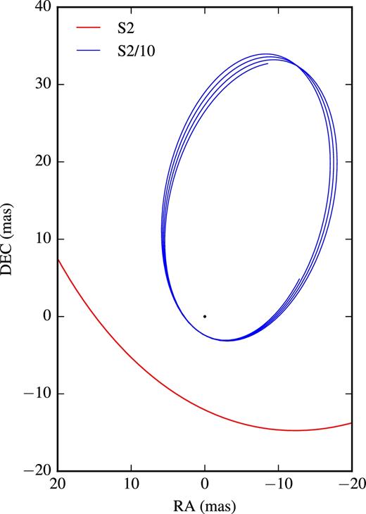
Example of Schwarzschild precession for the hypothetical star ‘S2/10’ during 5 yr. A portion of the S2 orbit is also shown.
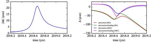
Left: The effect of light bending during periastron passage of S2 peaks at |${\approx } 20\, \mu$|as 12 d after periastron. This is the difference between an orbit with and without light bending. Right: Effect of periastron shift alone and with light bending around periastron passage of S2. Light bending enhances the periastron ‘kink’ and could help in the early detection of the combined effect, before having to wait for the continuous growth in the years following periastron passage. In both cases, the curves are the difference between the relativistic (without or with light bending) and the Keplerian orbits.
3.2 Photon orbit
In order to test the implementation of our solution for the photon orbit, we computed the effect of light bending on the astrometric position of the star S2. This is done by computing the difference |$|\sqrt{{\rm RA}^2+{\rm D{ec.}}^2}|$| as a function of time between bent and non-bent photon orbits. As shown in Fig. 2, the effect amounts to a deviation of |${\approx } 20\, \mu$|as during periastron passage. This is consistent with previous results (Bozza & Mancini 2012; Grould et al. 2017). In Fig. 2, we also show the superimposed effects of periastron shift and light bending; the latter amplifies the former during the periastron ‘kink’, enhancing the chances of an early detection of the combined effect.
3.3 Spin effect
We also computed the equivalent spin effects on the redshift. Again, the spin-angle dependence and size of the effects (0.01–0.3 and 3–30 km s−1 per orbit for S2 and S2/10, respectively) are consistent with Yu et al. (2016).
4 REQUIRED ORBITAL PARAMETERS FOR A BLACK HOLE SPIN MEASUREMENT
4.1 Simulated stellar orbits
The astrometric deviations due to spin cited above were calculated as the difference between models with zero and maximum black hole spin when keeping all other parameters (initial positions and velocities of the star, BH mass, and distance) constant. In practice, such parameters are not exactly known and have to be fit together with the black hole spin, which leads to masking of the spin-related effects.
We simulate stellar orbits across a grid of (aorb, e), with aorb ∈ (200RS, 5000RS) and e ∈ (0.1, 0.9). The other Keplerian parameters (ω, Ω, iorb) are taken to be the same as for S2. They only matter in relation to the black hole spin angles as far as spin-related effects are concerned. We choose ispin = εspin = 0°, which give astrometric shifts close to the average over the spin angles (specifically, 9.6 and |$31.7 \, \mu$|as per orbit for S2 and S2/10, respectively, compared to the averages of 8.5 and |$27.5 \, \mu$|as referred above). We use χ = 0.9 and the canonical MBH and R0 as above. The observing campaign is set to a total duration of T = 4 yr, with observations taken in three consecutive months per year over a period of 10 consecutive days per month, for a total of Norb = 120 observations. Gaussian errors with σx = 10 and |$100 \, \mu$|as are added representing canonical astrometric accuracies that could be achieved with GRAVITY.
In order to find the best-fitting zero-spin solution, we used a downhill simplex algorithm (Nelder & Mead 1965) which does not require numerical derivatives (as opposed to gradient methods such as Levenberg–Marquardt) and was found to be more stable and less sensitive to local minima. The method is based on constructing simplexes (polytopes of n + 1 vertices in n dimensions) and updating the vertices with operations (reflection, expansion, contraction, shrinkage) which result in successively better solutions. Because the method is not completely immune to local minima, we used 10 initial simplexes distributed around the initial parameters for each fit. This number was found to be sufficient in order to avoid local minima. We also note that no priors were used for MBH and R0. Even though they are constrained by the currently known S-stars, the best-fitting zero-spin solution is always within a few per cent of the initial value and therefore the currently known bounds would not lead to a change in significance.
4.2 Results
Fig. 3 (top row) shows the resulting significance contours σ(aorb, e) for |$\sigma _x = 10 \, \mu$|as. The graininess arises due to different error instantiations between simulated orbits. There is a region of low spin significance (σ ≲ 2) and of high spin significance (σ ≳ 5) separated by a relatively narrow transition region. The white contour lines show analytic estimates for the shape of this region based on equation (11).
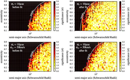
Contour plots for the significance σ of a black hole spin detection through monitoring of stellar orbits as a function of (aorb, e) for an observing campaign of 4 yr with a total of N = 120 observations. The black hole normalized spin is χ = 0.9 and spin angle parameters that lead to an average astrometric deviation are assumed. The white lines show the expected contour for astrometric deviations due to spin effects, aorb(1 − e2)3/4 = constant, which separates the regions of low and high significance. The left-hand panels show σ before finding the best-fitting zero-spin solution, i.e. simply setting χ = 0, whereas the right-hand panels show σ after fitting for the best zero-spin solution. The upper panels are for a purely astrometric campaign with precision |$\sigma _x = 10\, \mu$|as, while the lower panels contain additional radial velocity measurements with precision σrv = 50 km s−1. Having to fit all parameters leads to masking of the spin-related relativistic effects and leads to more stringent limits on the required star for a spin detection. The additional radial velocity measurements do not lead to an increase in significance before fitting, but help with constraining the non-spin parameters during the fit, ameliorating their masking of the spin effects.
The left-hand panel shows the significance before fitting, i.e. using the initial parameters but setting χ = 0, whereas the right-hand panel shows the significance after finding the best-fitting zero-spin solution. The pure size of the effect would suggest a star with aorb(1 − e2)3/4 ≲ 900RS is needed to detect spin at high significance, but in practice when fitting for all parameters a star with aorb(1 − e2)3/4 ≲ 300RS (i.e. ∼3 × closer in) is required.
4.3 Expected number of stars
In order to translate the constraint on orbital parameters from the previous section into an expected number of stars for which GRAVITY would be able to detect black hole spin, it is necessary to estimate the probability densities of semimajor axis, n(aorb), and eccentricity, n(e), and the K-band luminosity function (KLF, |$\frac{{\rm d}\log N(K)}{{\rm d}K} = \beta$|) in the central 1 arcsec/0.04 pc.
The latter has been estimated by several works with the consistent result β ≈ 0.20 (Genzel et al. 2003; Buchholz, Schödel & Eckart 2009; Sabha et al. 2012). The most recent analysis of the S-stars orbits is consistent with a ‘thermal’ eccentricity distribution (Gillessen et al. 2017); we therefore adopt n(e) de = 2e de. For such a distribution, if the energy distribution function follows a power-law, f(ε) ∝ εp, then the space density distribution n(r) ∝ r−γ and |$n(a_{\rm orb}) \propto a_{\rm orb}^{-\gamma +2}$| (Schödel et al. 2003). Estimates of γ from stellar counts in the region r ≲ 10 arcsec consistently find γ ≈ 1.2–1.4 (Genzel et al. 2003; Schödel et al. 2007; Do et al. 2009). We therefore adopt |$n(a_{\rm orb})\, {\rm d}a_{\rm orb} \propto a_{\rm orb}^{0.7} \,{\rm d}a_{\rm orb}$|, which is also in accord with the estimated semimajor axis distribution directly from the orbits of S-stars (Gillessen et al. 2009).
As mentioned, we set amax = 10 arcsec since n(aorb) would otherwise diverge. There is evidence from stellar counts that γ ∼ 2 for r > 10 arcsec (Genzel et al. 2003; Schödel et al. 2007; Fritz et al. 2016), so that n(aorb) = constant for r > 10 arcsec. Furthermore, beyond the radius of influence of the black hole ∼75 arcsec (Alexander 2005, we also note the direct measurements of a half-light radius of the nuclear star cluster ∼100 arcsec/178 arcsec by Schödel et al. (2014) and Fritz et al. (2016)), the orbits are significantly perturbed and not dominated by the gravitational potential of the black hole anymore. To check whether the chosen amax leads to a bias, we simulate the contribution from stars with 10 arcsec < aorb < 75 arcsec to the region r < 1 arcsec, which is found to be |${\lesssim } 1\,\,\rm{per\,\,cent}$|, since stars that do have the potential to reach r < 1 arcsec due to their higher eccentricities spend a very small portion of their orbital periods in this region.
We choose K < 19 as the upper limit on a star which could be detected with GRAVITY (Eisenhauer et al. 2011). The simulation predicts ∼1 such star within a radius r < 50 mas (∼ FOV of GRAVITY), in agreement with previous estimates (Genzel et al. 2003). The median (aorb, e) of such a star from the simulations is ≈(80 mas, 0.8). Because we have included the eccentricity distribution, we can also predict the expected number of stars that satisfy the contours for measuring spin derived in the previous section. We include an additional cut-off in aorb in order to ensure that at least one orbit is covered by the observing campaign (aorb < 5000RS for T = 4 yr).
Table 1 shows the expected number of stars which would allow a detection of spin. The masking of the relativistic effects by other parameters (‘Fit’ versus ‘No Fit’) leads to a significant reduction in the expected number of stars. For our canonical observing campaign of T = 4 yr, Nobs = 30 × 4 = 120 and |$\sigma _x = 10\, \mu$|as, we expect 0.035 star that would allow a significant detection of black hole spin. The median (aorb, e) of such stars is ≈(1200RS, 0.95).
Expected number of stars with K < 19 within given contour regions for measuring black hole spin for an observing campaign of duration T with 30 observations/yr, χ = 0.9 and spin angle parameters that lead to an average astrometric deviation.
| No Fit | Fit | Fit | |
|---|---|---|---|
| T = 4 yr | T = 4 yr | T = 10 yr | |
| |$\sigma _x = 10 \, \mu$|as No rv | 0.15 | 0.035 | 0.12 |
| |$\sigma _x=10 \, \mu$|as σrv = 50 km s−1 | 0.15 | 0.07 | 0.23 |
| No Fit | Fit | Fit | |
|---|---|---|---|
| T = 4 yr | T = 4 yr | T = 10 yr | |
| |$\sigma _x = 10 \, \mu$|as No rv | 0.15 | 0.035 | 0.12 |
| |$\sigma _x=10 \, \mu$|as σrv = 50 km s−1 | 0.15 | 0.07 | 0.23 |
We note that more recent papers have studied the faint population of stars in the Galactic Center in more detail, both using stellar counts going down to fainter limits (Gallego-Cano et al. 2018) as well as the faint diffuse light (Schödel et al. 2018). It is important to compare the estimated numbers above (which used assumptions on the stellar population based on brighter stars) to the ones based on the faint population alone. They found σ0 = 20 stars arcsec−2 and σ0 ∼ 72 stars arcsec−2 at R0 = 0.25 arcsec for stars with 17.5 ≤ K ≤ 18.5 and 18.5 ≤ K ≤ 19.5, respectively, and a surface density exponent Γ ∼ −0.4. From that we estimate ≈0.5 and ≈2 stars within 50 mas in the two magnitude ranges above, compared to the ≈1 star with K < 19 we found before. In this case, it is possible that our numbers above are pessimistic to within a factor of ∼2. We also note that Schödel et al. (2018) and Gallego-Cano et al. (2018) conclude that the population of faint stars is likely to be dominated by the old star population, and in that case a possible faint star found by GRAVITY is more likely to be part of the old cusp rather than a faint, typically young S-star of type A.
One of the consequences of equation (10) is that increasing T and Nobs or decreasing σx does not strongly increase the limit on aorb(1 − e2)3/4 (and therefore the number of stars). If we instead consider an observing campaign of 10 yr with Nobs = 30 × 10 = 300 total observations, then using equation (10) (and requiring aorb < 9000RS so that at least one orbital period is covered), the expected number of stars for measuring black hole spin increases to 0.12, with the median (aorb, e) of such stars ≈(2400RS, 0.96). The fraction of such stars with aorb > 5000RS (for which a spin measurement would very likely start to suffer from Newtonian perturbations) is |${\approx } 25\,\,\rm{per\,\,cent}$|.
We can also use these scalings to estimate the potential of future extremely large telescopes for measuring black hole spin from stellar orbits. The main advantage is the large increase in sensitivity. Assuming a limit K < 22, the numbers above should be multiplied by a factor of 4 based on the KLF. However, if the astrometric precision cannot reach the |$10\, \mu$|as level, the number of stars would be reduced accordingly. Also, if such telescopes could reach radial velocity precisions ∼1–10 km s−1 on faint stars, those could also be used to probe the black hole spin. Because the radial velocity changes are strongest near periastron (as opposed to apastron for the astrometric changes), they should be more robust to Newtonian perturbations (e.g. Psaltis et al. 2016). Finally, in the case of a large FOV there is the possibility of measuring relativistic effects from the collective motions of many further out stars (e.g. Do et al. 2017), but such an approach may be a challenge for measuring spin due to Newtonian perturbations.
We note that these estimates should be taken with caution since they are based on an extrapolation to the very inner region around the black hole which has been beyond the resolution limits of any instrument before GRAVITY. A cusp of massive stars in the immediate vicinity of the black hole (Alexander & Hopman 2009), precursors of stellar-mass black holes, for example could increase the expected number. Alternatively, a break in the KLF from bursts of star formation history (Pfuhl et al. 2011) could decrease it.
5 EFFECT OF RADIAL VELOCITIES
In the above analysis for detecting black hole spin, we have not so far considered radial velocity measurements, which could potentially be made by measuring the redshifts of spectral lines as is traditionally done for S-stars in the Galactic Center (Gillessen et al. 2009). In order to probe redshift effects on a stellar orbit due to spin, however, a very high redshift precision would be needed. As mentioned above, the maximum redshift difference (assuming the most optimistic spin angles) over a full orbit between models with χ = 0 and χ = 0.99 is ≈0.3 and 30 km s−1 for S2 and S2/10, respectively. The effect is also extremely sharped around periastron passage, and would require very targeted observing campaigns in order to be detected.
Previous work (Zhang et al. 2015; Yu et al. 2016) assumed redshift errors 1–10 km s−1 combined with astrometry when estimating spin errors. Such precision allows redshift probes of spin for potential stars in close orbits around SgrA*, but could only be achieved with future facilities such as E-ELT or TMT (Do et al. 2017). Current redshift measurements for the star S2 (significantly brighter than any potential close star, Gravity Collaboration 2017) have uncertainties ∼30 km s−1. Therefore, a natural question to ask is the extent to which potential radial velocity measurements with errors σv > 30 km s−1 could help in detecting spin. Although such precision would likely not be enough to measure spin by itself, it should help in better constraining the other parameters and therefore prevent the masking of spin effects to some extent, alleviating the constraints on the required stellar orbits.
Besides direct spectroscopy, we suggest a potential method to measure radial velocities of close orbit stars directly with GRAVITY using spectral differential interferometry in medium resolution. The method is outlined in Appendix A and we estimate a radial velocity precision σv ∼ 50 km s−1. In order to test the effect of adding the radial velocity measurements, we selected two example orbits near the transition region in Fig. 3, (aorb, e) = (500RS, 0.3) and (1600RS, 0.9), corresponding to a(1 − e2)3/4 ≈ 460RS, and ran a series of 240 fits using (i) only astrometric measurements with |$\sigma _x = 10 \, \mu$|as; (ii) astrometric and radial velocity measurements with |$\sigma _x = 10 \, \mu$|as and σv = 50 km s−1; and (iii) same as previous but with |$\sigma _x = 50 \, \mu$|as. The latter covers the case of radial velocity measurements at the expense of astrometric precision. Fig. 4 shows the histograms for the significance σ of spin detection for each case. The spread in σ (related to the graininess of the contour plots shown before) is natural due to the different error instantiations. A clear trend is observed, in the sense that adding the radial velocities increases the significance of a spin detection only if the astrometric precision can be maintained. Otherwise, if the astrometric precision is degraded by a factor of a few, the significance is severely lessened as the radial velocities themselves do not probe spin effects, but rather lead to a better constraint on the other parameters. Moreover, the increase in significance when adding radial velocities is stronger for the more eccentric orbit.
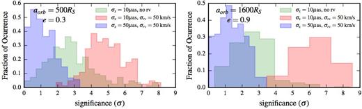
Effect of radial velocity measurements on the significance σ of black hole spin. We used the canonical observing campaign discussed previously, selected two orbits near the contour line (a(1 − e2)3/4 ≈ 460RS) of the upper right plot of Fig. 3, and ran 240 simulations to determine the significance after finding the best-fitting zero-spin solution. This was repeated for three cases: only astrometry with |$\sigma _x = 10\, \mu$|as (i), and including radial velocity measurements with σrv = 50 km s−1 with (ii) and without (iii) degradation of the astrometric precision to |$\sigma _{x}=50\, \mu$|as. The spread in σ for each case is due to the different error instantiations. Adding radial velocity measurements increases the significance by better constraining the orbital parameters, as long as the astrometric precision can be maintained. Notice also that the increase in σ due to radial velocities is more pronounced for the eccentric orbit.
In order to estimate how the required number of stars changes when including radial velocities, we created (aorb, e) contour plots with the same parameters as before but with additional redshift measurement σrv = 50 km s−1 at each observation. The result is shown in Fig. 3 (lower row) and Table 1. Whereas the contour line does not change before fitting for the zero-spin solution (since radial velocities with this precision are not probing spin effects), it does move outwards after performing the zero-spin solution fit, consistent with the behaviour observed in the two specific examples above. For the canonical observing campaign we use, this means aorb(1 − e2)3/4 ≲ 500RS, with the expected number of stars increasing by a factor of 2–0.07. Increasing the observing campaign to T = 10 yr increases the number of stars to 0.23.
6 DISCUSSION AND CONCLUSION
In this paper, the main goal was to determine the requirements that a hypothetical star would need to satisfy in order to allow a detection of black hole spin through the astrometric monitoring of its orbit around the supermassive black hole in the Galactic Center. In order to do this, we made use of a semi-analytical Kerr geodesics code to calculate stellar orbits close to SgrA*. Given the sparse sampling of the orbits and the large number of simulations needed, avoiding the numerical integration of the orbits leads to a significant improvement in computational time. For the photon orbit, because the spin effects on both astrometry and redshift are negligible compared to realistic precisions, we have used a weak-field Schwarzschild approximation.
We tested the validity of our code by checking it reproduces the expected relativistic effects on the star S2 and a hypothetical star S2/10. In particular, we noticed that the light bending when S2 passes behind the black hole during periastron passage enhances the signature from periastron advance and could lead to an early detection of the combined effect.
We have also shown the effect that radial velocities with precision ∼50 km s−1 would have in the detection of spin. Although such redshift precision does not allow to probe spin directly, it helps by providing stronger constraints on the other parameters. The number of expected stars increases by a factor of 2 if radial velocities at this precision are also available. It is therefore important to consider the possibility of radial velocity measurements in parallel to astrometry, and we give an example of a potential method to do this with GRAVITY.
In the above analysis, we have assumed that the black hole always lies at the origin. In practice, fitting S-star orbits requires the inclusion of offset and linear drift parameters of the black hole (Boehle et al. 2016; Gillessen et al. 2017). In the case of GRAVITY, astrometric measurements are taken relative to a reference star that is used to fringe track (Eisenhauer et al. 2011). Detecting relativistic effects would then require measuring its orbital parameters. However, Gravity Collaboration (2017) showed that it may be possible to reference stellar positions directly to SgrA*, removing the need for reference frame parameters as long as the near-infrared emission originates close to the black hole. In the case of upcoming extremely large telescopes, the results obtained here still apply except that the reference frame parameters should be included.
We have assumed a pure Kerr metric for the space–time around SgrA*, corresponding to the most optimistic case. In practice, a distribution of stars/remnants introduces perturbations that could mask the precession due to black hole spin. Even though these two effects could potentially be separated (e.g. astrometric deviations due to spin are maximum at apastron whereas Newtonian perturbations peak during periastron, Zhang & Iorio 2017), disentangling them with limited observations and without prior knowledge on the perturbers would be very challenging. From the diffuse light background from faint stars that cannot be currently resolved, Schödel et al. (2018) estimated a total enclosed stellar mass of ∼180 M⊙ within 250 mas. Using their measured 3D power-law density profile γ ≈ 1.1, this translates to only ∼2 M⊙ within 25 mas. From fig. 1 of Merritt et al. (2010), this would put an upper limit on aorb ∼ 10 000RS for frame dragging dominating over Newtonian perturbations, which the stellar orbits considered in this paper are well within. However, both theoretical considerations as well as simulations predict an accumulation of stellar-mass black holes (∼10 M⊙) in a steep cusp (γ ≈ 1.75–2.0) close to SgrA* through mass segregation (Freitag, Amaro-Seoane & Kalogera 2006; Hopman & Alexander 2006; Alexander & Hopman 2009; Preto & Amaro-Seoane 2010; Amaro-Seoane & Preto 2011). Current upper limits on the total mass within 25 mas (1.3 × 10⁵ M⊙, Boehle et al. 2016) or 13 mas (4 × 10⁴ M⊙, Gillessen et al. 2017) from fitting of stellar orbits cannot exclude the presence of a more massive dark cusp, and therefore it is important to consider its potential disturbance for the measurement of black hole spin with a closer star.
Both Merritt et al. (2010) and Zhang & Iorio (2017) consider a variety of stellar/remnant distributions with different perturber masses, total masses and density profiles to compare the effect of Newtonian perturbations to black hole precession. While Merritt et al. (2010) used N-body simulations to study the overall evolution of an entire cluster, Zhang & Iorio (2017) studied the detailed evolution of a test star in response to the perturbers. We can use their results to assess how much a black hole spin measurement for our two example stars in Section 5 with (aorb, e) = (500RS, 0.3) and (1600RS, 0.9) would suffer from Newtonian perturbations for different cluster properties. Considering stars with e = 0.88 and e = 0.3 with χ = 1 and spin angles such that the spin-induced astrometric changes are average (as we consider here), Zhang & Iorio (2017) find that the critical semimajor axes are 1440–2040RS and 1200–1560RS for a cluster of 10 M⊙ black hole perturbers with density profile γ = 1.75 and total mass of 30 and 100 M⊙ within 25 mas, respectively. Therefore, the more eccentric star would start to suffer from Newtonian perturbations for cluster masses ≳100 M⊙. Since Zhang & Iorio (2017) found that the effect of Newtonian perturbations is much less dependent on eccentricity than frame dragging, the advantage of a more eccentric star in terms of allowing for a larger semimajor axis is balanced by a higher sensitivity to Newtonian perturbations. Alternatively, from fig. 3 of Merritt et al. (2010), for a cusp of 10 M⊙ black holes with γ = 2 and a total mass ≲100 M⊙ within 25 mas and χ = 1, the critical radius is ≳5000RS, assuming the most optimistic black hole spin angles. Although the exact value depends on the black hole spin parameters, these results show that a steep cusp of black holes with total mass ≳100 M⊙ within 25 mas could start to compromise the measurement of black hole spin with a potential closer star.
Other methods could also be used to detect the black hole spin of SgrA*. Pulsar timing could reach much higher precision (e.g. Liu et al. 2012; Psaltis et al. 2016; Zhang & Saha 2017), but the lack of ordinary pulsar detections in deep surveys of the central parsec (Johnston et al. 1995; Macquart et al. 2010; Wharton et al. 2012; Dexter & O'Leary 2014) poses a significant challenge to this approach. Direct imaging of emission surrounding the ‘black hole shadow’ of SgrA* with radio VLBI (Doeleman et al. 2009; Falcke, Melia & Agol 2000; Goddi et al. 2017) could also potentially constrain spin, but so far suffers from complicated model-dependence (e.g. Broderick et al. 2009; Dexter, Agol & Fragile 2009). Finally, depending on the mechanism behind the NIR flares of SgrA*, astrometric monitoring of e.g. an orbiting hotspot could also allow a measurement of spin (e.g. Broderick & Loeb 2006; Hamaus et al. 2009; Vincent et al. 2011). All these methods are complementary. Although each is challenging, their combination could probe the space–time around SgrA* on scales ranging from ∼1 to 3000 Schwarzschild radii.
ACKNOWLEDGEMENTS
JD thanks Yang & Wang (2014) for making the ynogkm code public and D. Psaltis and J. Stone for useful discussions. This work was supported in part by a Sofja Kovalevskaja Award from the Alexander von Humboldt Foundation of Germany. OP acknowledges the support from ERC synergy grant No. 610058 ‘BlackHoleCam: Imaging the Event Horizon of Black Holes’. SG and PP acknowledge the support from ERC starting grant No. 306311.
REFERENCES
APPENDIX A: MEASURING RADIAL VELOCITIES OF A FAINT STAR WITH GRAVITY
Here, we explore the possibility of measuring radial velocities of a faint star with GRAVITY using differential visibility signatures across spectral lines. This would require the use of medium resolution (R ≈ 500). Although low resolution (R ≈ 22) has been the envisioned mode of operation in the Galactic Center due to SNR considerations, a bright flare state (K ∼ 15) or partial coupling of S2 (K ≈ 14) into the GRAVITY fibre (Gravity Collaboration 2017) could provide the necessary SNR for medium resolution, together with long integration times.
A possible faint star is expected to have absorption lines in its spectrum. The faintest early-type stars observed spectroscopically in the Galactic Center (K ≲ 17.5) are compatible with a A0/B9V classification and contain a Brγ absorption line (Pfuhl et al. 2011). For a fast moving star with vr ∼ 10 000 km s−1, such a line would be significantly displaced from its rest wavelength; therefore, discovering differential visibility signatures at unexpected wavelengths could allow to identify such stars and measure their radial velocity. We focus on an early-type star since they dominate the current spectroscopically identified stars in the S-star cluster (Eisenhauer et al. 2005; Habibi et al. 2017); however, we note that late-type giants are also a possibility for faint stars (Pfuhl et al. 2011), and could very well dominate the population of faint stars close to the centre (Gallego-Cano et al. 2018; Schödel et al. 2018). In the latter case, the series of sharp CO bands could provide even more convincing differential visibility signatures.
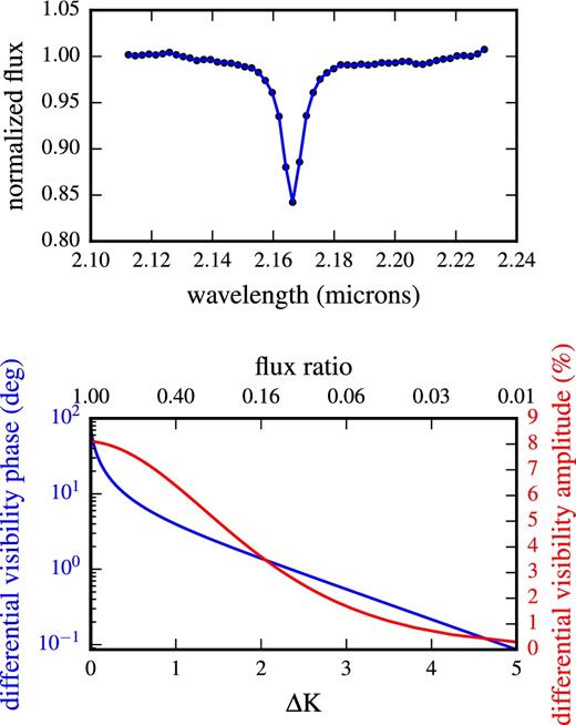
Top: Brγ line of an A0V star (Wallace & Hinkle 1997) with sampling appropriate to GRAVITY's medium resolution (R = 500) mode. Bottom: Maximum differential visibility phase and amplitude across a spectral line for a binary as a function of the flux ratio or near-infrared K-band magnitude difference. We assume a line depth 0.85 of the continuum corresponding to the spectrum above.
While the maximum differential visibility amplitude is |${\approx } 8\,\,\rm{per\,\,cent}$|, the differential visibility phase is strongly non-linear and could be >80° for an equal-brightness binary. Such a large signature could be used, for example, to test whether the quiescent emission from SgrA* has a contribution from a stellar component.
Here, we consider the case ΔK = 2 (|$f=16\,\,\rm{per\,\,cent}$|), which could correspond for e.g. to a faint star K = 18 with a brighter component (flare or S2). We set the binary separation σ = (10, 10) mas and onsider again the above case for the Brγ line with depth 0.85. Fig. A2 shows the differential visibility amplitude and phase as a function of |$\boldsymbol {u}\cdot \boldsymbol {\sigma }$|, as well as the points sampled by the six VLTI UT baselines, simulated assuming LST = 18 h as appropriate for observing the Galactic Center. The maximum differential phase and amplitude signals are ≈1.5° and |$4\,\,\rm{per\,\,cent}$|, respectively. GRAVITY has already achieved a differential precision 0.2°/|$0.4\,\,\rm{per\,\,cent}$| and 0.5°/|$1\,\,\rm{per\,\,cent}$| on K ≈ 6 and K ≈ 10 sources with short integration times ∼1 h, respectively (Gravity Collaboration 2017).
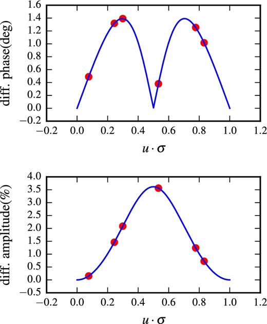
Differential visibility phase and amplitude across the Brγ spectral line as a function of |$\boldsymbol {u}\cdot \boldsymbol {\sigma }$| for the case ΔK = 2. The six red points show a possible sampling with the VLTI UT baselines with binary separation vector σ = (10, 10) mas.
In order to estimate the radial velocity precision that could be potentially achieved with such a method, we simulate differential signals on the six baselines assuming precisions σϕ = 0.3° and |$\sigma _{{\rm amp}} = 0.6\,\,\rm{per\,\,cent}$|, and fit all baselines simultaneously with Lorentzian profiles for the differential signatures. The resulting statistical error in redshift is σrv ≈ 30 km s−1. Considering additional systematic errors of comparable order, we adopt σrv = 50 km s−1 for our simulations.
