Gravitational instability and star formation in NGC 628

Abstract

1 INTRODUCTION

The disc gravitational instability is often thought to play an important role in the large-scale star formation in galaxies. The theory of this subject is well developed (Quirk 1972; Jog & Solomon 1984; Elmegreen 1995; Efstathiou 2000; Rafikov 2001; Romeo & Wiegert 2011; Romeo & Falstad 2013) and the existence of the relationship between disc instability and star formation was demonstrated by observations (Kennicutt 1989; Hunter, Elmegreen & Baker 1998; Boissier et al. 2003; Leroy et al. 2008; Romeo & Wiegert 2011; Hunter et al. 2013; Zheng et al. 2013; Yim et al. 2014; Romeo & Fathi 2015, 2016; Hallenbeck et al. 2016; Garg & Banerjee 2017; Romeo & Mogotsi 2017) and simulations (e.g. Li, Mac Low & Klessen 2005, 2006; Goldbaum, Krumholz & Forbes 2015, 2016; Inoue et al. 2016; Fiacconi et al. 2017). Recent investigations (e.g. Krumholz, Dekel & McKee 2012) have shown that this link is rather indirect. The processes involved in the formation of stars are multiple, very complex and operate on atomic to galactic size scales (see e.g. McKee & Ostriker 2007). Even so, the regions, which are gravitationally unstable according to the simple one-fluid gravitational criterion by Goldreich & Lynden-Bell (1965), can be rather easily calculated and compared with the regions of the ongoing star formation (Kennicutt 1989; Hunter et al. 1998; Martin & Kennicutt 2001).

The predictions of gravitational instability diagnostics are not always accurate. For example, half of galaxies in the sample by Martin & Kennicutt (2001) demonstrate the perceptible star formation rate (SFR) and stable gaseous discs. One reason is that stars affect the instability level and a gaseous disc should be considered with stellar one simultaneously, as was shown by Jog & Solomon (1984). Another reason lies in the fact that real galaxies are not axisymmetric systems and this effect is very difficult to take into account in the instability analysis. Finally, most of the works mentioned examine one-dimensional data, which are placed along the spectrograph's long slit (e.g. Marchuk & Sotnikova 2018) or more often azimuthally averaged (e.g. Kennicutt 1989; Hunter et al. 1998; Boissier et al. 2003; Leroy et al. 2008). As galaxies usually demonstrate non-axisymmetric or irregular structure and a small filling factor for gas, azimuthally averaged data can lead to large uncertainties. There are a small number of works which examine data maps, rather than one-dimensional data profiles (Yang et al. 2007; Elson, de Blok & Kraan-Korteweg 2012), because applying gravitational instability criterion needs many independent types of observational data or various assumptions if data are missed.

Even in the era of massive integral field unit (IFU) surveys, galaxies with all available data of interest are rare, because these surveys either cover only central parts of galaxies or have low spatial resolution. NGC 628 is one of the few exceptions. It is close, face-one well-studied galaxy, which is listed in many surveys. Instability analysis in Leroy et al. (2008) (hereafter L08) shows that azimuthally averaged disc is marginally stable within r < 0.5r₂₅ and can be unstable at r > 0.5r₂₅. At the same time, a lot of star-forming regions are located in central parts of the galaxy. Thus, NGC 628 is a good candidate to apply reasonable two-component model and find how the model can predict the location of star-forming areas, which are scattered unevenly across the disc. Recently, Dib, Hony & Blanc (2017) have done similar analysis for almost the same data cubes, but they applied a modified criterion using Larson scaling laws and only focused on the SFR prediction. They also treated stars as an isothermal fluid and took only 90 data points with a lower resolution of 750 pc.

In this work, the relationship between two-component gravitational instability and large-scale star formation for NGC 628 using a small number of assumptions and a huge number of data points in the galaxy image is investigated. The performed analysis is similar to that in previous work of Marchuk & Sotnikova (2018). In Section 2, the data sources and necessary formulas are presented along with short method description. Section 3 contains obtained results and discussion about them.

2 DATA AND METHOD

NGC 628 (M74) is an SA(s)c galaxy with two grand-design spiral arms. The galaxy is visible almost face-on under inclination i = 7°. Herrmann et al. (2008) compared different estimates of the distance and found that D = 8.6 Mpc is the most accurate estimate (see fig. 5 in Herrmann et al. 2008 and more recent paper by Kreckel et al. 2017), while L08 used D = 7.3 Mpc. In this work, more precise 8.6 Mpc distance and scale 24 arcsec kpc⁻¹ are used. The galaxy visual size is r₂₅ = 294 arcsec according to L08. NGC 628 was studied intensively and included in more than 1200 works according to NASA ADS. A complete overview of other unmentioned properties may be found in Zou et al. (2011) and references therein.

Provided analysis is based on VENGA (Blanc et al. 2013a,b) data cubes and utilizes the same area sized 5.2 × 1.7 arcmin across the centre. It extends to 1–2 exponential stellar scales in every direction from the galaxy centre assuming the exponential scale value is equal to 65 arcsec (L08). In paragraphs below, every type of needed data is described and conversion formulas are given. For comparison reasons, data conversion methods in this work follow a scheme by L08 except the formulas for the velocity dispersion of stars.

|${H\,\small {I}\ data}$|⁠. Both atomic hydrogen surface densities |$\Sigma _{\mathrm{H\, \small {I}}}$| and velocity dispersions |$\sigma _{\mathrm{H\, \small {I}}}$| were obtained using THINGS (Walter et al. 2008) data cube. In this work, the data cube with a natural weighting (NA) is used, which has a size equal to 1024 × 1024 pixels and a spatial resolution equal to 1.5 arcsec, or 62 pc. The integrated intensity was converted into |$\Sigma _{\mathrm{H\, \small {I}}}$| according to formula (A1) from L08. The procedure includes helium correction factor 1.36. Obtained |$\Sigma _{\mathrm{H\, \small {I}}}$| and |$\sigma _{\mathrm{H\, \small {I}}}$| maps were compared with images in Walter et al. (2008) and L08 and found to be exactly the same. The maximal atomic hydrogen velocity dispersion value in the area of interest was around 23 km s⁻¹ and the mean value was close to 11 km s⁻¹, which L08 used as a constant sound speed value for both atomic and molecular gases.

A first moment map from THINGS was also used to construct a ‘cold’ gas rotation curve υ_c. Velocities along the major axis were extracted from the cube, bent across the centre, and corrected for the inclination and systemic velocity. The obtained profile was fitted by the cubic smoothing spline up to 200 arcsec. The resulting υ_c fit shown in Fig. 1 is in good agreement with the results of other works by Suwannajak, Tan & Leroy (2014), Herrmann & Ciardullo (2009), and Vollmer & Leroy (2011), among which only the latter demonstrates the rotation curve which is long enough.

Figure 1.

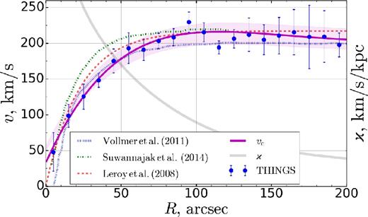
Rotation curve. Points with errors represent THINGS velocity data, averaged over 10 arcsec bins. Solid magenta line shows gas rotation curve υ_c fit. Solid grey line shows epicyclic frequency ϰ. Other types of lines represent various approximations from the literature.

Open in new tabDownload slide

The rotation curve was used to calculate the epicyclic frequency |$\varkappa = \displaystyle \sqrt{2}\frac{\upsilon _\mathrm{c}}{R}\sqrt{1+\frac{R}{\upsilon _\mathrm{c}}\frac{\text{d}\upsilon _\mathrm{c}}{\text{d}R}}$|⁠, which is also presented in Fig. 1. The derivative in this formula was calculated numerically and tested for stability by another fit using small degree polynomial and by using data from Vollmer & Leroy (2011). As ϰ, we actually use an azimuthally averaged characteristic. But there is no inconsistency in this approach. The epicyclic frequency is a derivative of the rotation curve, which, in turn, is a characteristic of the total potential. The potential is determined not by local fluctuations of the gas density, but by global massive subsystems.

H₂ data. Molecular gas surface densities were derived from HERACLES map (Leroy et al. 2009) in the line CO(J = 2 → 1). This map was obtained using beam size 13.6 arcsec. Molecular gas follows spiral arms pattern (fig. 17 in Leroy et al. 2009). HERACLES map for NGC 628 demonstrates better sensitivity than data of BIMA-SONG (Helfer et al. 2003) and CARMA (Rahman et al. 2012) surveys (see fig. 1 in Blanc et al. 2013b). This figure also shows good agreement between all three surveys. The formula (A3) from L08 was used to convert intensities into |$\Sigma _\mathrm{H_2}$|⁠, where a constant CO-to-H₂ factor X_CO = 2 × 10²⁰ cm⁻² (K km s⁻¹)⁻¹ was assumed and resulting densities were corrected for helium. Map for part of analysed region from Rebolledo et al. (2015) demonstrates values similar to those obtained here for H₂. It should be noted that it is difficult to compare obtained map directly with central upper map in L08. While azimuthally averaged |$\Sigma _\mathrm{H_2}$| profile is similar with that in L08 (see table 7 in L08 for exact values), the same is not true for |$\Sigma _\mathrm{H\, \small {I}}$| profile. The source of this difference is unclear. It seems that in fig. 35 in L08 one profile was corrected for helium and another was not (see Fig. 2 in comparison). In this work, non-constant CO-to-H₂ gradients from Blanc et al. (2013b) were also tested.

Figure 2.

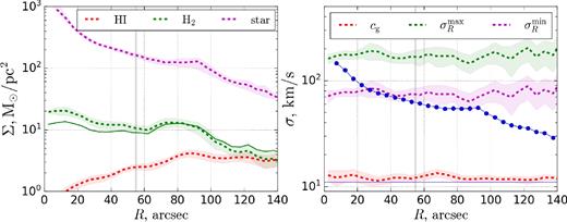
Azimuthally averaged profiles for calculated data, where dashed lines represent mean values and filled areas show three standard deviations. Annuli are formed for 5 arcsec bins. Left plot shows surface densities Σ and right plot shows velocity dispersions σ. Gaseous densities are not corrected for helium. Vertical grey line demonstrates radius of last full annulus (55 arcsec). Solid green line on the left shows change in mean |$\Sigma _\mathrm{H_2}$| for another CO-to-H₂ conversion factor (see the text). Points on the right show σ_R from L08 and horizontal line shows commonly accepted level c_g = 11 km s⁻¹.

Open in new tabDownload slide

A molecular gas velocity dispersion map was found only in Wilson et al. (2011) with inappropriate resolution. A comparison of radially averaged dispersions |$\sigma _{\mathrm{H\, \small {I}}}$| and σ_CO in Mogotsi et al. (2016) and Caldú-Primo et al. (2013) suggests that both components are well mixed and justifies to use |$\sigma _\mathrm{H_2}=\sigma _{\mathrm{H\, \small {I}}}$|⁠. The colder molecular gas with |$\sigma _{\mathrm{H\, \small {I}}} = 1.5\times \sigma _\mathrm{H_2}$| was also tested for a three-component model (see below).

Stellar surface density. Stellar surface densities Σ_s were obtained using the same technique as in L08. They adopt a constant mass-to-light ratio in K band equal to 0.5 M_⊙/L_{⊙, K} and then apply an empirical conversion from |$3.6\,\rm{\mu m}$| to K-band intensity using formula (C1). L08 calculated stellar surface densities using data from SINGS (Kennicutt et al. 2003), while in this analysis the same formula was applied to more recent |$3.6\,\rm{\mu m}$| data from S⁴G (Sheth et al. 2010). A spatial resolution of data is near the same as in THINGS and is equal to 1.66 arcsec. A resulting Σ_s map agrees well with a radial profile in L08 if azimuthal averaging is used (fig. 35 in their work and Fig. 2 here). Note that a more precise method for surface densities estimation from |$3.6\,\rm{\mu m}$| (e.g. Querejeta et al. 2015) has been introduced recently, but it is difficult to compare directly with previous results.

SFR. L08 suggested to use FUV data along with |$24\,\rm{\mu m}$| line intensity as an SFR tracer. In this work corrected for dust, an H α map from Blanc et al. (2013b) was used instead. This map has the same spatial resolution and size as VENGA data cube. Formula (2) from Murphy et al. (2011) was used for the map conversion into SFR. Blanc et al. (2013b) also provide an SFR map constructed from FUV and |$24\,\rm{\mu m}$| data, which shows good agreement with the H α map, but has a slightly lower resolution. L08 also found that both methods coincide well.

Azimuthal profiles. Azimuthally averaged profiles for calculated data are shown in Fig. 2. The uncertainty in these profiles was calculated using formula (E1) from L08 and beam size for VENGA data cubes. It can be seen that relative scatter in surface densities is rather small in comparison with velocity dispersions. Note that Σ profiles are in good agreement with L08 data except |$\mathrm{H\, \small {I}}$| and that σ_R velocity dispersions from L08 follow lower boundary of |$\sigma _R^{\mathrm{min}}$| in this work. Notice also that all annuli for R > 55 arcsec constructed not for the whole ellipses due to rectangular form of area under consideration. Probably this is the reason why scatter increased for large distances.

Method. From all data cubes described above, the same VENGA rectangle was extracted (see fig. 1 in Blanc et al. 2013a). Then coordinates of the centre of a 155 × 55 pixels grid in the VENGA cube were found and all needed data (⁠|$\Sigma _{\mathrm{H\, \small {I}}}$|⁠, |$\sigma _{\mathrm{H\, \small {I}}}$|⁠, |$\Sigma _\mathrm{H_2}$|⁠, Σ_s, |$\sigma _{R}^\mathrm{max}$|⁠, |$\sigma _{R}^\mathrm{min}$|⁠, Σ_SFR, ϰ) were collected for each pixel. In following instability analysis, pixels masked as foreground stars in VENGA cube were not used. In order to avoid the bulge influence, all points closer than the bulge effective radius r_b,eff = 15 arcsec (Möllenhoff & Heidt 2001; Fisher & Drory 2010; Zou et al. 2011) were excluded from the analysis. Finally, outer regions R > 140 arcsec of extracted area were also excluded because of significant uncertainties.

3 RESULTS AND DISCUSSION

Fig. 3 demonstrates the results of gravitational instability diagnostics for NGC 628. The two-component model with smaller stellar radial dispersions |$Q_\mathrm{eff}^\mathrm{min}$| shows a good agreement with observed star formation for a threshold |$Q_\mathrm{eff}^\mathrm{min} < 2\hbox{--}3$| all over the area studied. On the other hand, the parameter Q_g for gas only can explain star formation for distant areas R > 80 arcsec but shows a stable disc inside this radius. The model with |$Q_\mathrm{eff}^\mathrm{max}$| represents an intermediate case between two mentioned. Unstable regions follow the spiral arms, which according to Foyle et al. (2010) just gather more gas inside and are not a trigger of star formation themselves.

Figure 3.

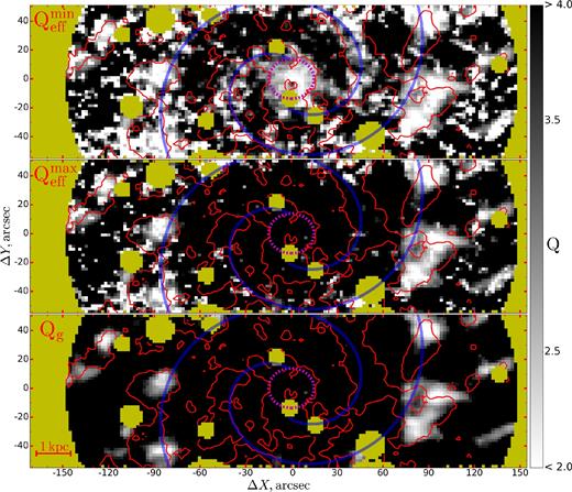
Q-parameter for two components with |$\sigma _R^\mathrm{min}$| (upper), |$\sigma _R^\mathrm{max}$| (middle), and gas-only (lower) models. Star-forming regions Σ_SFR > 0.007 M_⊙ yr⁻¹ kpc⁻² are shown by red contours. Masked stars are yellow. Bulge effective radius (magenta dashed) and logarithmic spirals (transparent blue, parameters from Gusev & Efremov 2013) are marked.

Open in new tabDownload slide

3.1 Uncertainties

Correctness and stability of obtained results were tested in several ways. The analysis performed is correct only for a short-wavelength approximation, which should be checked. Even taking into account that some star-forming areas show the most unstable wavelength λ ≈ 3 kpc, corresponding regions always have the same or large length at least at one direction, as can be seen in Fig. 4 for |$Q_\mathrm{eff}^\mathrm{min}$| model. Secondly, uncertainties of Q were checked. For H₂ and σ_los, error values are given in separated data cubes. For |$\Sigma _{\mathrm{H\, \small {I}}}$|⁠, the uncertainties were taken equal to 1 M_⊙ pc⁻² as THINGS sensitivity limit. The rotation curve was varied within 7 per cent to account for differences between approaching and receding parts (transparent area in Fig. 1). Stellar surface density uncertainties were obtained by varying the mass-to-light ratio for the K band within 0.48–0.6 M_⊙/L_⊙ as L08 suggested. Applying all uncertainties together did not affect the results much and a root mean square error in Q levels changes is around 15 per cent.

Figure 4.

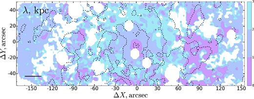
The most unstable wavelengths λ in kpc for |$Q_\mathrm{eff}^\mathrm{min}$| model. Three different levels up to 3 kpc are shown. White areas demonstrate masked stars or regions with λ > 3 kpc. Black dashed lines represent areas of star formation. Black segment in the lower left corner shows a 1 kpc linear scale.

Open in new tabDownload slide

A common weakness in all such diagnostics is the adoption of a constant conversion factor X_CO, since it can significantly change (Oka et al. 1998; Pineda et al. 2010). Fortunately, an attempt to measure the radial profile of X_CO was done in Blanc et al. (2013b) and Aniano et al. (2012). The resulting stability levels were tested using the results by Blanc et al. (2013b), as the authors mention large uncertainties in Aniano et al. (2012) and caution against accepting a single X_CO. Both provided profiles of X_CO for their parameters N = 1 and N = 1.5 almost coincided within the uncertainties and led to a change in the conversion factor of about 50 per cent, making it smaller in the centre and larger outside (see solid line in Fig. 2, left subplot). Despite the noticeable changes in |$\Sigma _\mathrm{H_2}$|⁠, taking into account the gradient X_CO does not significantly affect the values of Q, but slightly decreases it on the periphery. The next paragraph can shed light on this behaviour.

Disc thickness can significantly affect the disc stability and makes it more stable (Romeo & Wiegert 2011; Romeo & Falstad 2013). In order to account for this effect, the approximation with individual components for atomic and molecular gas as in equation (19) in Romeo & Falstad (2013) was used. This approximation shows a good accuracy (see e.g. Marchuk & Sotnikova 2018). Two cases |$\sigma _{\mathrm{H\, \small {I}}} = \sigma _\mathrm{H_2}$| and |$\sigma _{\mathrm{H\, \small {I}}} = 1.5\times \sigma _\mathrm{H_2}$| were tested. A comparison between Q_RF obtained for three-component thick model and exact Q_eff for a thin disc shows noticeable change. Taking thickness into account makes |$Q_\mathrm{RF}^\mathrm{min}$| close to |$Q_\mathrm{eff}^\mathrm{max}$| and |$Q_\mathrm{RF}^\mathrm{max}$| becomes similar to Q_g for both gas dispersion suggestions. Fig. 9 partially demonstrates this results, where |$Q_\mathrm{RF}^\mathrm{min}$| is plotted. However, the thickness stabilization effect can be compensated by the dissipation effect (Elmegreen 2011) up to its complete neglection in extreme cases. Unfortunately, the dissipation effect is hard to account for. Note that used approximation from Romeo & Falstad (2013) can also show which component is most unstable. In central parts of NGC 628, stars determine the dynamic status of a disc while molecular gas determines the instability for outer parts where Q_g model works well. This is the reason of result in previous paragraph, where change in CO-to-H₂ factor does not affect the central parts.

3.2 Star formation relations

Some well-known facts about star formation (Kennicutt & Evans 2012) were also tested. First one is the so-called Kennicutt–Schmidt star formation law (Schmidt 1959; Kennicutt 1989), which describes the relationship between SFR and the total gas density in |$\Sigma _\mathrm{SFR} \propto \Sigma _\mathrm{g}^{N}$| form, where N = 1.4–1.5 (Kennicutt 1989). This and other relations are shown in Fig. 5. Kennicutt–Schmidt law on the left subplot is fulfilled with large scatter. It probably shows some evidences of more complex behaviour due to bended form. Best-fitting line is shown for N = 1.48.

Figure 5.

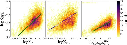
Star formation laws. All plots represent point counts in hexagon binning with 50 bins. Left plot shows original Kennicutt–Schmidt law; line slope is 1.48. Central plot shows the same law for molecular gas only, dashed line represents a constant depletion time t_dep = 2 Gyr. On the right image dependence proposed in Ostriker, McKee & Leroy (2010) is shown; line slope is 1.

Open in new tabDownload slide

Central plot in Fig. 5 demonstrates an expected correlation between star formation and the amount of molecular gas. Values |$\Sigma _\mathrm{H_2}$| on this plot are corrected for helium presence. Clearly Kennicutt–Schmidt law in NGC 628 is determined by molecular gas mostly. Also, expectation about no clear correlation between SFR density and atomic hydrogen is held (Bigiel et al. 2008). No pixels were found with |$\Sigma _{\mathrm{H\, \small {I}}}$| higher than 10 M_⊙ pc⁻², which is known as hydrogen molecularization threshold, as can be seen in Fig. 2.

Many other forms of Kennicutt–Schmidt law were developed in recent works. They are found from observations fits like |$\Sigma _\mathrm{SFR} \propto \Sigma _\mathrm{g}^{1.13\pm 0.05}\Sigma _\mathrm{s}^{0.36\pm 0.04}$| (Shi et al. 2011), |$\Sigma _\mathrm{SFR} \propto (\Sigma _\mathrm{s}^{0.5}\Sigma _\mathrm{g})^{1.09}$| (Shi et al. 2018) as well as from sophisticated models like |$\Sigma _\mathrm{SFR} \propto \Sigma _\mathrm{g} \Sigma _\mathrm{s}^{0.5}$| (Ostriker et al. 2010) or Σ_SFR ∝ Σ_gΣ_s (see references in Krumholz 2015). The trend suggested by model in Ostriker et al. (2010), where contribution to the vertical gravitational field of the stellar disc plays important role in star formation, was checked. This law for analysed data is represented on the right plot in Fig. 5. It shows smaller scatter than original Kennicutt–Schmidt relation. The good confirmation of this trend also has been found recently in Westfall et al. (2014).

Finally, the map of molecular gas depletion time was studied. Many recent works (Leroy et al. 2013 and references therein and in Kennicutt & Evans 2012) have found that depletion time to be almost constant, t_dep = 2 Gyr, and this value already often has been referenced as fiducial. In this work, selected star formation areas (see below) are in excellent agreement with regions of constant depletion time in Fig. 6. However, this only allows us to conclude that in selected areas of star formation all molecular gas can be consumed faster than 2 Gyr if recent SFR persists. This constant level t_dep=2 Gyr is also shown by a line for the central plot in Fig. 5.

Figure 6.

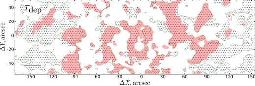
Molecular gas depletion time in comparison with star-forming areas. Colour filled areas correspond to the level Σ_SFR > 0.007 M_⊙ yr⁻¹ kpc⁻². Hatched regions correspond to t_dep < 2 Gyr. Black segment in the lower left corner shows a 1 kpc linear scale.

Open in new tabDownload slide

3.3 Azimuthal averaging

All tests suggest that obtained two-component model is reliable and can associate the observed star formation regions with Q ≈ 2–3 areas. However, this is not true if azimuthally averaged data are used. Azimuthal averaging is often used in works, because it has a physical justification that the whole disc is considered to be in an equilibrium state. Note, however, that the uneven distribution of gas has a little effect on the equilibrium, since its mass is relatively small. At the same time, regions with a larger gas density can be more unstable than others. Thus, spatial maps of the Q stability parameter, although not fully consistent with the axisymmetric approximation, are a useful complement to radial profiles of Q and can provide further insight between star formation and gravitational instability, for instance by revealing prominent local minima of Q that would be suppressed by azimuthal averaging. In Fig. 7, the same obtained results for models |$Q_\mathrm{eff}^\mathrm{min}$|⁠, |$Q_\mathrm{eff}^\mathrm{max}$|⁠, and Q_g are shown after azimuthal averaging procedure. Notice, how stable the discs become even within 55 arcsec, where annuli were formed correctly. The uncertainties of Q profiles are small and cannot affect the results. The disc for all models in Fig. 7 is stable, except central parts of |$Q_\mathrm{eff}^\mathrm{min}$| profile and the location of massive bright spirals at 90 arcsec. Such a stable disc does not allow predicting the location of star-forming regions.

Figure 7.

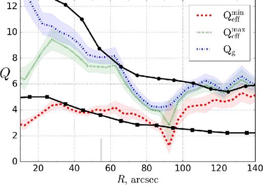
Azimuthally averaged profiles for Q data, where dashed lines represent mean values and filled areas show uncertainty, obtained for one standard deviation in data. Annuli are formed for 10 arcsec bins. Vertical grey segment on lower axis shows radius of the last full annulus (55 arcsec). Solid black lines show Q profiles from L08 for gas only (upper, circles) and for two-component (lower, squares) models.

Open in new tabDownload slide

To summarize, discs appear to be more stable after averaging. Even for |$Q_\mathrm{eff}^\mathrm{min}$| model mean values equal 3–4 almost everywhere except central region and spirals at 90 arcsec. Such artificially cold discs are not allowing to predict regions of star formation correctly and only usage of two-dimensional maps like in Fig. 3 can do it. Conclusion that azimuthal averaging can strongly affect the obtained values of Q should be fulfilled for galaxies similar to NGC 628, where the matter distribution is patchy.

3.4 Best match with SFR threshold

It is interesting to see how well the different instability levels can be associated with star-forming regions. This question addresses two threshold values Q_lim and |$\Sigma _\mathrm{SFR}^\mathrm{lim}$|⁠. The best matching between gravitationally unstable Q < Q_lim regions and noticeable star formation areas |$\Sigma _\mathrm{SFR} > \Sigma _\mathrm{SFR}^\mathrm{lim}$| is searched for. Thereafter, pixels with SFR density lower than threshold will be called ‘without signal’ and ‘with signal’ otherwise. Pixels where Q < Q_lim will be mentioned as ‘with predicted signal’ and ‘without predicted signal’ else. The whole problem was treated as a binary classification task where the exact values of Q or SFR in pixels are not important, but only agreement between signal presence or absence and its correct prediction.

Commonly accepted criteria for coincidence like χ² are not appropriate, because high Q_lim and low |$\Sigma _\mathrm{SFR}^\mathrm{lim}$| along with low Q_lim and large |$\Sigma _\mathrm{SFR}^\mathrm{lim}$| show better matching than intermediate values. This point is illustrated on the central subplot in Fig. 8, where solid lines represent ratio of correctly founded pixels for Q_lim = 3 case. This is so-called accuracy metric in machine learning field. It is equal to the number of matches between observations and model predictions (i.e. the number of pixels ‘with signal’ and ‘with predicted signal’ or ‘without signal’ and ‘without predicted signal’ accordingly) divided by number of pixels. Accuracy by definition cannot be larger than unity. From the central subplot in Fig. 8, it seems like Q_g model explains data better than two-component models for some |$\Sigma _\mathrm{SFR}^\mathrm{lim}$| thresholds. However, as mentioned above, this is not completely true, because areas with and without star formation are highly imbalanced for some thresholds values and one can actually get lower total error if predicts no star formation at all. This can be also seen from additional dashed lines on the same figure, which show how many star-forming regions are predicted well. This line represents so-called recall, which equals to the number of correctly predicted pixels with signal divided by the total number of pixels with signal. Obviously |$Q_\mathrm{eff}^\mathrm{min}$| model makes correct signal prediction more often than other models. Note that both types of lines converge on the left border, because there are no pixels without signal anymore and accuracy becomes the same as recall.

Figure 8.

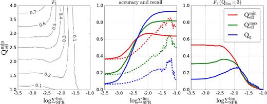
Lines of the best coincidence between star formation and gravitational instability thresholds. On the left picture F₁ score contour map for |$Q_\mathrm{eff}^\mathrm{min}$| model is shown. Central plot demonstrates accuracy (solid) and recall (dashed) scores for Q_lim = 3 (see the text for details). Colours are the same as for the right plot. On the right plot, F₁ scores with Q_lim = 3 are presented.

Open in new tabDownload slide

Thus, the problem of finding best match is not straightforward and needs to be balanced somehow for two types of errors: predicts nothing where signal exists and does not predict anywhere it actually is. One needs to find limits which lower both mentioned types of errors simultaneously. For this reason, a well-known machine learning approach was used instead. These limits are searched in order to maximize so-called F₁ score, which represents balanced metric and equals to harmonic mean between precision (ratio of correctly predicted pixels with signal to the total number of pixels with predicted signal) and recall for predicted and observed classes (Rijsbergen 1979). An additional limitation is that a correction for non-axisymmetric perturbations cannot lead to the Q threshold larger than 3 (see e.g. Marchuk & Sotnikova 2018 and references therein).

Measured F₁ scores for different |$Q_\mathrm{eff}^\mathrm{min}$| levels are shown in the left plot in Fig. 8. The higher score is better. It can be seen from the plot that increasing Q_lim allows us to find higher score. As possible Q_lim values are limited by an upper value, one should search the best score for Q_lim = 3 case. Corresponding F₁ scores for all models are shown on the right plot in Fig. 8. As expected, one-fluid model is less precise than two-component model and |$Q_\mathrm{eff}^\mathrm{min}$| shows higher scores than |$Q_\mathrm{eff}^\mathrm{max}$|⁠. Last mentioned model demonstrates maximum for log Σ_SFR ≈ −2.25. Better model |$Q_\mathrm{eff}^\mathrm{min}$| did not reveal clear maximum score, but became flat at level F₁ ≈ 0.56 after log Σ_SFR ≈ −2.5, which means that model does not become better for lower |$\Sigma _\mathrm{SFR}^\mathrm{lim}$| thresholds. Taking into account that solid accuracy line for |$Q_\mathrm{eff}^\mathrm{min}$| model on the left plot shows maximum near log Σ_SFR ≈ −2.0, it must be concluded that best searched match should lie between −2.5 and −2.0 boundaries.

Hence, the best obtained fit is for |$Q_\mathrm{eff}^\mathrm{min}$| model with Q_lim = 3 and |$\Sigma _\mathrm{SFR}^\mathrm{lim}=0.007\, \mathrm{M}_{\odot }$| yr⁻¹ kpc⁻², which is the average value between boundaries above. Star formation contours in all map figures (Figs 3, 4, 6, 9) in this work are also not arbitrary and represent this best fit. Corresponding areas for best match thresholds are shown in Fig. 9. Notice a good agreement between the model and observations even inside the bulge effective radius. As before, the gaseous disc alone can explain star formation only in outer regions even for Q_g ≈ 3. Note also that unstable regions according to |$Q_\mathrm{eff}^\mathrm{max}$| model lie inside those for |$Q_\mathrm{eff}^\mathrm{min}$| model and |$Q_\mathrm{RF}^\mathrm{min}$| model is similar to |$Q_\mathrm{eff}^\mathrm{max}$| one as was mentioned above. Two-component model of gravitational instability |$Q_\mathrm{eff}^\mathrm{min}$| can correctly explain selected regions of star formation for a vast radii range. An implicit evidence that founded match is reasonable also comes from depletion time map agreement.

Figure 9.

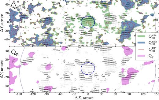
Levels of the best coincidence between star formation and gravitational instability. Upper plot shows data for two-component models and bottom for gas only. Colour filled areas and red contours correspond to the level Q ≤ 3 of the appropriate model. Hatched regions correspond to Σ_SFR > 0.007 M_⊙ yr⁻¹ kpc⁻². Bulge effective radius is marked by the dashed blue line and the area R ≤ 140 arcsec is enclosed by the blue solid line.

Open in new tabDownload slide

4 SUMMARY

In this work, a large number of two-dimensional data were collected for grand-design galaxy NGC 628 and the connection between two-component gravitational instability and large-scale star formation was analysed. An additional support for such relationship came from recent works about self-shielding (Orr et al. 2017; Stark et al. 2018) and from idea of global Toomre regime (Krumholz et al. 2012). A small number of assumptions were used and the performed analysis is mainly similar to that in previous work of Marchuk & Sotnikova (2018), but adjusted for maps. Various tests of obtained results were performed including azimuthal averaging and accounting for disc thickness effect. Some star formation relations were testified. The best explainable |$\Sigma _\mathrm{SFR}^\mathrm{lim}$| threshold was found.

In summary, next results were obtained:

• the two-component gravitational instability model for NGC 628 shows a good agreement with observable large-scale star formation;

• previous result also stays true if the model is accounted for X_CO gradients or disc thickness effect;

• the parameter Q_g for gas-only model can explain star formation only in distant regions and thus, the destabilizing effect of a stellar component cannot be neglected;

• an azimuthal averaging procedure makes disc more stable and cannot predict the location of star-forming regions;

• the relationship between disc instability and star formation is perhaps tighter than currently believed at least for one model;

• the largest area of star formation in NGC 628 which can be explained by gravitational instability is determined by the condition |$\Sigma _\mathrm{SFR}^\mathrm{lim}>0.007\, \mathrm{M}_{\odot }$| yr⁻¹ kpc⁻².

ACKNOWLEDGEMENTS

Author thanks Alessandro Romeo for his great review and highly appreciate the comments and suggestions that significantly contributed to improving the quality of this paper. Author is grateful to Guillermo Blanc for providing VENGA data and acknowledge the hard work of the THINGS, HERACLES, S⁴G, and VENGA teams and thanks them for making their data publicly available.

This research makes use of the NASA/IPAC Extragalactic Database (NED) which is operated by the Jet Propulsion Laboratory, California Institute of Technology, under contract with the National Aeronautics and Space Administration and the LEDA data base (http://leda.univ-lyon1.fr).

REFERENCES