


Abstract
The δ Sct stars are a diverse group of intermediate-mass pulsating stars located on and near the main sequence within the classical instability strip in the Hertzsprung–Russell diagram. Many of these stars are hybrid stars pulsating simultaneously with pressure and gravity modes that probe the physics at different depths within a star's interior. Using two large ensembles of δ Sct stars observed by the Kepler Space Telescope, the instrumental biases inherent to Kepler mission data and the statistical properties of these stars are investigated. An important focus of this work is an analysis of the relationships between the pulsational and stellar parameters, and their distribution within the classical instability strip. It is found that a non-negligible fraction of main-sequence δ Sct stars exist outside theoretical predictions of the classical instability boundaries, which indicates the necessity of a mass-dependent mixing length parameter to simultaneously explain low and high radial order pressure modes in δ Sct stars within the Hertzsprung–Russell diagram. Furthermore, a search for regularities in the amplitude spectra of these stars is also presented, specifically the frequency difference between pressure modes of consecutive radial order. In this work, it is demonstrated that an ensemble-based approach using space photometry from the Kepler mission is not only plausible for δ Sct stars, but that it is a valuable method for identifying the most promising stars for mode identification and asteroseismic modelling. The full scientific potential of studying δ Sct stars is as yet unrealized. The ensembles discussed in this paper represent a high-quality data set for future studies of rotation and angular momentum transport inside A and F stars using asteroseismology.
1 INTRODUCTION
The δ Sct stars are a diverse group of pulsating stars found at the intersection of the main sequence (MS) and the classical instability strip in the Hertzsprung–Russell (HR) diagram, which corresponds to spectral types between A2 V and F2 V for MS Population I stars, and effective temperatures approximately between 6400 ≤ Teff ≤ 8600 (Breger 2000b; Rodríguez & Breger 2001; Aerts, Christensen-Dalsgaard & Kurtz 2010; Uytterhoeven et al. 2011). This places δ Sct stars within an interesting transition region in the HR diagram between low-mass stars with radiative cores and thick convective envelopes (M ≲ 1 M⊙) and high-mass stars with large convective cores and radiative envelopes (M ≳ 2 M⊙) – see Bowman (2017) for a recent review of δ Sct stars. The observations of the physical properties of δ Sct stars provide useful constraints for stellar structure and evolutionary models, since the physical properties such as interior rotation, and the size and shape of the convective core have a significant impact on the evolution of intermediate and massive stars (Maeder 2009; Meynet et al. 2013).
The observation and modelling of stellar pulsations – known as asteroseismology – provides insight of the interior physics of stars for a wide range of stellar masses and evolutionary stages across the HR diagram (Aerts et al. 2010). The pulsation modes excited within a star are dependent on stellar structure, thus pulsation mode frequencies provide direct insight of physics within a star where traditional methods in astronomy, such as photometry and spectroscopy, are unable to probe directly. This makes asteroseismology unique, with its strong observational constraints of stellar physics used for improving theoretical models of stellar structure and evolution. The dominant pulsations in δ Sct stars are self-excited by the opacity (κ) mechanism operating in the He ii ionization zone (Cox 1963; Breger 2000b; Aerts et al. 2010), which produces pressure (p) modes with periods as long as 8 h and short as 15 min (Uytterhoeven et al. 2011; Holdsworth et al. 2014). These p modes typically have low radial orders and are most sensitive to the surface layers of a star. Another form of coherent mode excitation in δ Sct stars is from turbulent pressure, which is able to excite p modes with radial orders between 7 ≤ n ≤ 10 with higher pulsation mode frequencies for stars within the classical instability strip (Houdek 2000; Antoci et al. 2014; Xiong et al. 2016).
The instability regions of the δ Sct and the lower mass γ Dor stars are predicted to overlap in the HR diagram (Dupret et al. 2004, 2005; Houdek & Dupret 2015), with stars that simultaneously pulsate in p modes excited by the κ mechanism and gravity (g) modes excited by the convective flux blocking (modulation) mechanism commonly referred to as hybrid stars. The exact nature the excitation mechanism of g modes and its physical relationship with the κ mechanism in intermediate-mass stars is not fully understood (see e.g. Xiong et al. 2016), with a significant fraction of δ Sct stars hotter than the γ Dor instability region observed to pulsate with g modes (Uytterhoeven et al. 2011; Bowman 2016, 2017). Few hybrid stars were known prior to space photometry (see e.g. Handler 2009). The unprecedented photometric precision, duty cycle, and total length of the Kepler mission (Borucki et al. 2010; Koch et al. 2010) revealed that many δ Sct stars are hybrid stars (Grigahcène et al. 2010; Uytterhoeven et al. 2011; Balona & Dziembowski 2011; Balona 2014). On the other hand, it is also demonstrably true that pure δ Sct stars with no significant frequencies below 5 d−1, albeit rare, exist (Bowman 2017).
An analysis of 750 A and F stars was carried out by Uytterhoeven et al. (2011) using 1 yr (Q0–Q4) of Kepler data, and it was concluded that approximately 25 per cent were hybrid pulsators. Later analyses of A and F stars using longer time spans of Kepler data by Balona (2014) and Balona, Daszyńska-Daszkiewicz & Pamyatnykh (2015) have found much higher fractions of δ Sct stars with low frequencies in their amplitude spectra, but also demonstrate that less than 50 per cent of stars within the classical instability strip pulsate. This measured incidence of pulsation amongst δ Sct stars should be considered a lower limit with 50 per cent of A and F stars observed to pulsate using the detection threshold Kepler photometry, which is of order a few |$\mu$|mag in the best of cases. For many A and F pulsators, it is not established if observed low-frequency peaks are caused by pulsation modes, rotational modulation, combination frequencies, or have some other astrophysical cause (Bowman 2017). Recent studies by Van Reeth, Tkachenko & Aerts (2016) and Saio et al. (2018) have discovered that global normal modes of Rossby waves (r modes), which cause temperature perturbations in a rotating star, are visible in A and F stars in the Kepler data set. Specifically, r modes in rapidly rotating γ Dor stars exhibit a power excess at low frequency, such that r modes with azimuthal order m produce a group of frequencies slightly below m times a star's rotation frequency (Saio et al. 2018).
For chemically normal stars within the classical instability strip, it is not surprising that they are observed to pulsate from the nature of the driving mechanism in δ Sct stars (Murphy et al. 2015), although it is also known that approximately half of stars within the classical instability strip are not pulsating (Balona & Dziembowski 2011) at the photometric precision of order a few |$\mu$|mag in Kepler data. Further work is needed to study the interplay between the flux blocking mechanism and the κ mechanism in A and F stars, with a focus on understanding the synergy between the pulsation excitation mechanisms and the observed minority of δ Sct stars pulsating in purely p modes. This provides motivation for characterizing the pulsation properties of a large ensemble of δ Sct stars observed by Kepler presented in this work.
However, one of the main difficulties encountered when observing δ Sct stars is the issue of identifying pulsation modes in terms of their radial order, n, angular degree, ℓ, and azimuthal order, m. The typical low-order p modes in δ Sct stars often do not show any regular spacing in the amplitude spectrum, unlike the asymptotic high radial order p modes in low-mass solar-type stars – see Chaplin & Miglio (2013) and Hekker & Christensen-Dalsgaard (2017) for reviews of solar-like pulsators. The rapid rotation, mode visibility, and our incomplete understanding of mode excitation in δ Sct stars make them one of the more challenging groups of pulsating stars to study using asteroseismology (e.g. Reese et al. 2017). Despite these complexities, ongoing efforts to apply ensemble asteroseismology techniques to δ Sct stars are being made using similar methods to those used to study low-mass stars (García Hernández et al. 2009, 2013, 2015; Paparó et al. 2016; Michel et al. 2017).
Significant progress in understanding the physics of δ Sct stars has been made since the space photometry revolution facilitated by the COROT (Auvergne et al. 2009) and Kepler (Borucki et al. 2010) space missions. The rich pulsation spectra of δ Sct stars offer the potential to probe physics at different depths using asteroseismology, thus these stars can provide useful constraints of stellar structure and evolution theory in an important transition region on the MS (Breger 2000b; Aerts et al. 2010). The full scientific potential of studying pulsation modes in δ Sct stars with asteroseismology in the era of space photometry has yet to be exploited.
1.1 Regularities in the amplitude spectra of δ Sct stars
It has been the goal of various studies to search for regularities in the amplitude spectra of δ Sct stars (e.g. García Hernández et al. 2009, 2013, 2015; Paparó et al. 2016; Michel et al. 2017), with a particular focus of identifying the asymptotic frequency separation between modes of consecutive high radial order, known as the large-frequency separation Δν. However, δ Sct stars often have high-mode densities in their amplitude spectra caused by dozens, and sometimes hundreds, of pulsation mode frequencies making it difficult to distinguish intrinsic pulsation modes. This is complicated by non-linearity of pulsation modes in δ Sct stars in the form of harmonics, nνi, and combination frequencies, nνi ± mνj, where n and m take integer values (Pápics 2012; Kurtz et al. 2015; Bowman 2017). These non-linear combination frequencies can have high Fourier amplitudes but do not represent intrinsic pulsation modes since they describe the non-sinusoidal shape of a star's light curve in the Fourier domain, and can also create regularities in an amplitude spectrum (see chapter 6 from Bowman 2017).
Recently, Michel et al. (2017) searched for regularity in the amplitude spectra of 1860 δ Sct stars observed by COROT, using two observables which they termed fmin and fmax corresponding to the lower and upper limits for significant frequencies in a star's amplitude spectrum. Michel et al. (2017) define significant frequencies as those that have an amplitude larger than 10 times the mean amplitude in an amplitude spectrum. A subsample of approximately 250 of these stars were classified as young δ Sct stars since they had high-frequency pulsation modes with |$f_{\rm max} \ge 400 \, \mu$|Hz (≳35 d−1), such that they were consistent with theoretical modes of stars near the zero-age main sequence (ZAMS). Michel et al. (2017) found an agreement between the observed frequency distribution and the corresponding distribution caused by island modes from theoretical models using a non-perturbative treatment of fast rotation (Reese et al. 2009). Specifically, regularities in the amplitude spectra of these stars produced ridge-like structures with spacings of order a few tens of |$\, \mu$|Hz (of order a few d−1) consistent with consecutive radial order pulsation modes. Thus, the observables fmin and fmax were concluded to be potentially useful diagnostics to constrain the mass and evolutionary stage of a δ Sct star (Michel et al. 2017).
The ensemble approach of studying pulsating stars certainly has its advantages, especially for such diverse pulsators as δ Sct stars (Grigahcène et al. 2010; Uytterhoeven et al. 2011; Balona & Dziembowski 2011; Balona 2014; Bowman et al. 2016; Bowman 2017; Michel et al. 2017). In this paper, the statistical properties of a large number of δ Sct stars observed by the Kepler Space Telescope are investigated with a discussion of the target selection methods provided in Section 2, an evaluation of the edges of the classical instability strip presented in Section 3, an analysis of the correlations between the pulsational and stellar parameters given in Section 4, and the results for a search for regularities in the amplitude spectra given in Section 5. Finally, the conclusions are presented in Section 6.
2 COMPILING ENSEMBLES OF KEPLER δ S|$\bf ct$| STARS
The Kepler Space Telescope was launched on 2009 March 7 and has an Earth-trailing orbit with a period of 372.5 d (Borucki et al. 2010). Within its 115 deg2 field of view in the constellations of Cygnus and Lyra, it observed approximately 200 000 stars at photometric precision of order a few |$\mu$|mag (Koch et al. 2010). To maximize its goal of finding transiting Earth-like planets orbiting Sun-like stars, Kepler had two observing modes: a long cadence (LC) of 29.45 min and a short cadence (SC) of 58.5 s (Gilliland et al. 2010). From the limited onboard data storage capacity, only 512 stars could be observed in SC at a given epoch. The Kepler LC data were divided into quarters (from Q0 to Q17) covering a maximum length of 1470.5 d, whereas SC data were divided into 30-d segments, which was motivated by the rolling of the Kepler spacecraft and data downlink epochs approximately every 90 and 30 d, respectively. Kepler data are available from the Mikulski Archive for Space Telescopes (MAST1) in pre- and post-pipeline formats – see Smith et al. (2012) and Stumpe et al. (2012) for details of the Kepler science data pipeline. In this work, the post-pipeline data, known as multiscale Maximum A Posteriori Pre-search Data Conditioning (msMAP PDC) data, are used.
Previously, a large ensemble of 983 δ Sct stars with LC Kepler data was compiled by Bowman et al. (2016) to study amplitude modulation of pulsation modes. Later, Bowman (2016, 2017) used the same stars to investigate the relationship between the pulsation and stellar parameters in δ Sct stars. This ensemble of δ Sct stars was comprised of Kepler stars characterized by 6400 ≤ Teff ≤ 10 000 K in the Kepler Input Catalogue (KIC; Brown et al. 2011); were observed continuously in LC by Kepler for 4 yr; and had significant peaks in the p-mode frequency range (ν ≥ 4 d−1) with amplitudes above 0.10 mmag. Although an amplitude cut-off of 0.10 mmag is higher than the typical noise level observed for Kepler data, it was chosen by Bowman et al. (2016) to ensure that all extracted peaks had reasonable phase uncertainties, as these are dependent on the amplitude signal-to-noise (S/N) ratio (Montgomery & O'Donoghue 1999). The KIC ID numbers and stellar parameters such as effective temperature and surface gravity of these stars were provided as supplementary online data in Bowman et al. (2016), with a machine-readable table also available through CDS.
To evaluate the impact of these biases in the LC Kepler data for the analysis of δ Sct stars, specifically the amplitude visibility function suppressing high-frequency pulsation modes, a second ensemble of δ Sct stars compiled using SC Kepler data is also analysed independently in this work. The δ Sct stars in the SC ensemble of stars were selected using the same criteria as the LC ensemble, except no restriction was placed on the length of the SC data. The ensembles of SC and LC δ Sct stars have been filtered for known binarity using the Villanova binary catalogue2 (Prša et al. 2011; Abdul-Masih et al. 2016). It is important to note that δ Sct stars in eclipsing binaries and ellipsoidal variables have been excluded from the ensembles presented in this work because of the effects of contamination, which could significantly affect the Teff determination using photometry such as those included in the KIC (Brown et al. 2011).
These selection criteria produced an LC ensemble of 963 stars and an SC ensemble of 334 δ Sct stars. All stars in the LC ensemble have continuous Kepler observations spanning 4 yr, but the δ Sct stars in the SC ensemble have total time spans that range between 10 and 1470 d. The longest continuous light curve for each SC δ Sct star ranges between 10 and 1000 d, with approximately 50 per cent of stars having only 30 d of Kepler SC data. There are 218 stars that are duplicated in both ensembles, with 116 SC stars that are not included in the LC ensemble. It is easy to understand why additional SC δ Sct stars were not included in the LC ensemble, in terms of amplitude suppression from the amplitude visibility function given in equation (1), and because SC observing slots were at a premium during the Kepler mission. The duplicate stars are not removed from either ensemble, nor are the ensembles combined as each ensemble suffers from different biases which should not be compounded into unknown biases.
2.1 Extracting δ Sct stellar parameters
The vast majority of the 200 000 Kepler target stars were characterized with values of Teff and logg using griz and Two Micron All-Sky Survey (2MASS) JHK broad-band photometry in the KIC (Brown et al. 2011). This catalogue has since been revised by Huber et al. (2014) with values of Teff being accurate in a statistical sense for such a large number of stars.
High-resolution and high S/N spectroscopy using the HERMES spectrograph mounted on the Mercator telescope (Raskin et al. 2011) was obtained and analysed by Niemczura et al. (2015) for 117 bright (V ≲ 10 mag) A and F stars observed by Kepler. Accurate values for fundamental stellar parameters including Teff, logg, rotational and microturbulent velocities, and their respective uncertainties were determined for each star (Niemczura et al. 2015). An additional 44 A and F stars were also observed using the FIES spectrograph mounted on the Nordic Optical Telescope by Niemczura et al. (2017). Similar to the analysis by Huber et al. (2014), a 200 K systematic offset was found between the KIC and spectroscopic values of Teff (Niemczura et al. 2015, 2017) for A and F stars. High-resolution and high S/N spectroscopy of B, A, and F stars observed by Kepler was also obtained by Tkachenko et al. (2012, 2013) using the 2-m telescope of the Thüringer Landessternwarte Tautenburg in Germany.
However, not all the stars studied by Niemczura et al. (2015, 2017) and Tkachenko et al. (2012, 2013) are δ Sct stars, but those that are represent a subset of δ Sct stars for which accurate values of Teff and logg are known, with uncertainties for an individual star typically between 100 ≤ σ(Teff) ≤ 200 K and 0.1 ≤ σ(logg) ≤ 0.2 (cgs), respectively. Only 58 and 70 stars studied by Tkachenko et al. (2012, 2013) and Niemczura et al. (2015, 2017) are included in the LC and SC ensembles, respectively, but these stars are included in this work to show compatibility with the KIC and Huber et al. (2014) values.
2.2 Extracting δ Sct pulsation parameters
To characterize the pulsational properties for the δ Sct stars in both ensembles, the amplitude spectrum for each star was calculated from 0 ≤ ν ≤ 98 d−1, which has an upper frequency limit corresponding to four times the LC Nyquist frequency. The highest amplitude pulsation mode was extracted and optimized using a non-linear least-squares fit to the light curve using the function |$\Delta \,m = A\, \cos (2\pi \nu (t -t_0)+\phi )$|, where A, ν, and ϕ are the pulsation mode amplitude, frequency, and phase, respectively, calculated using the zero-point of the time-scale as t0 = 2 455 688.77 BJD. Each extracted pulsation mode frequency was checked to satisfy the commonly used significance criterion of S/N ≥ 4 in amplitude (Breger et al. 1993) and that it did not correspond to a known instrumental spurious frequency. 3 The amplitude spectrum over a large-frequency range for each star is useful for studying regularities in δ Sct stars, which is discussed later in Section 5.
By not correcting the amplitude spectra for the δ Sct stars in either ensemble for the amplitude visibility function given in equation (1) prior to extracting pulsation mode frequencies, it is ensured that the extracted peak is a pulsation mode frequency and not a Nyquist alias frequency, since Nyquist aliases have lower observed amplitudes than the corresponding real peaks (Murphy, Shibahashi & Kurtz 2013). Furthermore, this approach is to avoid dividing by zero for pulsation mode frequencies very close to the LC Kepler sampling frequency, which would cause some δ Sct stars to have extremely large and unphysical pulsation mode amplitudes. Instead, pulsation mode amplitudes are corrected for the amplitude visibility function after they have been extracted from an amplitude spectrum. The disadvantage of this approach is that the distribution of LC pulsation mode frequencies will be biased towards, on average, lower values, but this is a compromise that yields the most meaningful results. This also emphasizes the need to keep both ensembles of δ Sct stars separate in this analysis, since the amplitude visibility function has a negligible effect for stars in the SC Kepler ensemble.
3 REVISITING THE EDGES OF THE CLASSICAL INSTABILITY STRIP WITH KEPLER DATA
In this section, the observed boundaries of the classical instability strip are evaluated using the high-quality photometry provided by the Kepler Space Telescope using the two ensembles of δ Sct stars. Prior to space photometry from COROT and Kepler, evolutionary and pulsation models of δ Sct stars were calibrated to catalogues of δ Sct stars collated using ground-based observations, for example, Rodríguez & Breger (2001). Compared to space data, ground-based observations have higher noise levels and suffer from lower duty cycles and significant aliasing, which introduces strong selection effects when studying pulsating stars. These issues make it difficult to extract low-amplitude pulsation modes and thus a δ Sct star may be classified as a non-pulsating star from the ground if its pulsation mode amplitudes are lower than the noise level. Typically, the noise level in the amplitude spectrum of ground-based photometry is a few tenths of a mmag for a single observing site (e.g. Bowman et al. 2015; Holdsworth et al. 2018), but can be as low as tens of |$\mu$|mag in the best of circumstances (Kurtz et al. 2005). With Kepler data, we are afforded the luxury of 4 yr of continuous high-precision light curves resulting in a white-noise level of order a few |$\mu$|mag in an amplitude spectrum.
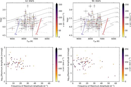
The distribution of the 963 LC and 334 SC δ Sct stars in Teff–logg diagrams using values from the KIC are shown in the top left and top right panels of Fig. 1, respectively. The location of each δ Sct star is shown by a black cross, with a typical error bar shown in bold in the bottom right corner of each panel. For comparison, the same ensembles using the revised parameters from Huber et al. (2014) are shown in bottom left and bottom-right panels of Fig. 1 as filled grey squares. Stellar evolutionary tracks using a metallicity of Z = 0.02 from Grigahcène et al. (2005), which are calculated from the ZAMS (indicated by a short-dashed purple line) to a post-MS effective temperature of Teff = 5900 K, for stars of 1.4, 1.8, 2.2, and 2.7 M⊙ are also shown in Fig. 1 as solid purple lines. The theoretical blue and red edges of the classical instability strip from Dupret et al. (2005) for radial p modes between 1 ≤ n ≤ 6 are shown as blue and red lines, with solid and dashed lines indicating the boundaries for n = 1 and 6 radial modes, respectively. The subgroup of δ Sct stars for which accurate spectroscopic values of Teff and logg from Tkachenko et al. (2012, 2013) and Niemczura et al. (2015, 2017) are also plotted as filled green circles in each panel with their respective 1σ uncertainties in Fig. 1.
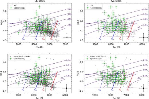
The Teff–logg diagrams for the ensemble of LC and SC δ Sct stars observed by Kepler are shown in the left- and right-hand panels, respectively. The locations of δ Sct stars using parameters from the KIC are shown by black crosses in the top row, and Huber et al. (2014) values are shown as grey squares in the bottom row, with a typical error bar shown in bold in the bottom right corner of each panel. Stellar evolutionary tracks using a metallicity of Z = 0.02 from Grigahcène et al. (2005) calculated between the ZAMS (shown as a short-dashed purple line) and a post-MS effective temperature of Teff = 5900 K are shown as solid purple lines. The subgroup of δ Sct stars with spectroscopic values of Teff and logg from Tkachenko et al. (2012, 2013) and Niemczura et al. (2015, 2017) are plotted as filled green circles. The theoretical blue and red edges of the classical instability strip from Dupret et al. (2005) for p modes with radial order of n = 1 are shown as solid blue and red lines, respectively, and radial order of n = 6 shown as dashed blue and red lines, respectively.
The majority of δ Sct stars shown in Fig. 1 are schematically consistent with the theoretical blue and red edges of the classical instability strip calculated by Dupret et al. (2005) if the lower and upper bounds of the uncertainties on Teff values are considered for hot and cool δ Sct stars, respectively. However, there is no evidence to indicate that temperatures of hot and cool δ Sct stars would be over- and underestimated in such a systematic fashion. When comparing the distribution of stars using the KIC and Huber et al. (2014) values in Fig. 1, it is clear that the Huber et al. (2014) values are shifted to temperatures approximately 200 K higher. However, this systematic increase in temperature of the Huber et al. (2014) compared to the KIC values produces more outliers beyond the blue edge. These outliers represent a small yet significant fraction of δ Sct stars in both ensembles, which includes stars with accurate spectroscopic Teff values obtained by Tkachenko et al. (2012, 2013) and Niemczura et al. (2015, 2017), that are significantly hotter than the blue edge for the n = 6 radial overtone p mode calculated by Dupret et al. (2005).
Many of the δ Sct stars in Fig. 1 have surface gravities between 3.5 ≤ logg ≤ 4.0, except for those near to the ZAMS and the red edge. Thus, the middle of the MS and the terminal-age main sequence (TAMS) are well sampled compared to the ZAMS for hot δ Sct stars observed by the Kepler Space Telescope. The high density of δ Sct stars shown in the left-hand panels of Fig. 1 that are near the ZAMS and red edge of the theoretical instability strip calculated by Dupret et al. (2005), implies that ZAMS stars cooler than Teff ≃ 6900 K are able to pulsate in p modes. Many of the outliers at the red edge of the classical instability strip can be explained as within 1σ of the classical instability strip, but equally importantly, many of these δ Sct stars are within 1σ of being cooler than the red edge. The lack of δ Sct stars with spectroscopic effective temperatures and surface gravities from Tkachenko et al. (2012, 2013) and Niemczura et al. (2015, 2017) that are cooler than the red edge is likely caused by a selection effect in these author's target lists.
A value of αMLT between 1.8 and 2.0 was determined to produce a reasonably good agreement between the theoretical models and observations of δ Sct stars by Dupret et al. (2004, 2005). However, it should be noted that the highest mass model used by Dupret et al. (2005) to investigate αMLT was 1.8 M⊙, but higher mass δ Sct stars exist within the Kepler data set, especially since stars with masses M > 2.7 M⊙ are included in Fig. 1 and have been confirmed by spectroscopy. It was discussed in detail by Dupret et al. (2005) that decreasing the value of αMLT to 1.0 has the effect of shifting the instability strip to lower values of effective temperature, and vice versa. Thus, a mass-dependent value of αMLT is needed to reproduce both the observed blue and red edges of the classical instability strip. It is important to note that the observed boundaries of the classical instability strip are purely empirical and are subsequently used to constrain theoretical models. Furthermore, the observed edges using ground-based observations of δ Sct stars, which span 7400 ≤ Teff ≤ 8600 K at logg ≃ 4.4 (Rodríguez & Breger 2001; Bowman 2017), are narrower than the theoretical boundaries shown in Fig. 1. Clearly, the theoretical red edge of the classical instability strip is more difficult to model compared to the blue edge because of the complex interaction of surface convection and the κ mechanism in cool δ Sct stars, with the convective envelope predicted to effectively damp pulsations in stars cooler than the red edge (Pamyatnykh 1999, 2000; Dupret et al. 2004, 2005; Houdek & Dupret 2015). These results indicate that further theoretical work is needed in understanding mode excitation in δ Sct stars, specifically those pulsating in higher radial orders (n ≥ 6), and the large temperature range of observed δ Sct stars.
In summary, it is concluded that a statistically non-negligible fraction of δ Sct stars are located cooler than the red edge and hotter than the blue edge of the classical instability strip calculated by Dupret et al. (2005), as shown in Fig. 1. A plausible explanation for the minority of δ Sct stars located outside of the classical instability strip using the KIC and Huber et al. (2014) values are that they have incorrect Teff and logg values, since these were determined using photometry, but outliers do exist with some stars having stellar parameters confirmed using spectroscopy. Therefore, these results demonstrate the need for a mass-dependent value of αMLT to reproduce all of the δ Sct stars observed by the Kepler Space Telescope. The δ Sct stars that lie outside the classical instability strip will be interesting to study further, as they lie in a region where the excitation of low radial order p modes by the κ mechanism is not expected to occur (Pamyatnykh 1999, 2000; Dupret et al. 2004, 2005).
4 CHARACTERIZING THE PULSATION PROPERTIES OF δ S|$\bf ct$| STARS OBSERVED BY KEPLER
In this section, correlations between the pulsation properties and stellar parameters of δ Sct stars are investigated using the LC and SC ensembles. The pulsation properties of δ Sct stars are diverse and, upon first inspection, little commonality is often found when comparing the amplitude spectra of individual δ Sct stars in terms of the number of excited pulsation modes, their amplitudes and the observed frequency range. Since the number of significant pulsation modes in δ Sct stars ranges from as small as a single mode4 to hundreds, it is difficult to characterize and compare the total pulsation energy in a systematic way for an ensemble of stars (Bowman 2016). This is complicated by the fact that the majority of δ Sct stars have variable pulsation mode amplitudes, with the total observable pulsational budget being unconserved on time-scales of order a few years (Bowman & Kurtz 2014; Bowman et al. 2016). Also, in a classical pre-whitening procedure, it is important to exclude harmonics and combination frequencies when quoting the range of observed pulsation mode frequencies as these frequencies are caused by the non-linear character of the pulsation modes and do not represent independent pulsation mode frequencies (Pápics 2012; Kurtz et al. 2015; Bowman 2017).
4.1 Pulsation mode amplitudes
Amongst the δ Sct stars, a subgroup of high-amplitude δ Sct (HADS) stars exists, which were originally defined by McNamara (2000) as δ Sct stars with peak-to-peak light amplitudes exceeding 0.3 mag. HADS stars are also typically slowly rotating (|$v$| sini ≲ 40 km s−1) and pulsate in the fundamental and/or first-overtone radial modes. These stars are known to be rare, making up less than one per cent of pulsating stars within the classical instability strip (Lee et al. 2008), but the physical cause of their differences to typical δ Sct stars remains unestablished, if any exists (Balona 2016).
To demonstrate the rarity of HADS stars in the Kepler mission data and examine the typical pulsation mode amplitudes in δ Sct stars, the (logarithmic) distributions of the amplitude of the highest amplitude pulsation mode for the LC and SC ensembles are shown in the top and bottom panels of Fig. 2, respectively. In each panel of Fig. 2, the amplitudes of the dominant pulsation modes have been approximately separated into p modes (ν ≥ 4 d−1) and g modes (ν < 4 d−1), and are showed as the filled grey and red areas respectively. It is possible for g-mode frequencies and combination frequencies of g modes to exceed 4 d−1, but typically they have lower amplitudes and do not represent the dominant pulsation mode in a star. Each amplitude is corrected for the amplitude visibility function given in equation (1), with the corrected distributions for p and g modes shown as the black- and red-hatched regions, respectively. As expected, the amplitude visibility function has a negligible effect on the SC ensemble. By separating δ Sct stars into if their dominant pulsation mode corresponds to g or p mode, it is demonstrated that a non-negligible fraction, more than 15 per cent, of δ Sct stars have their highest amplitude pulsation mode in the g-mode frequency range. We also investigated using a value of 7 d−1 to separate g- and p-mode-dominated δ Sct stars, which yielded similar results with a difference of order a few per cent.
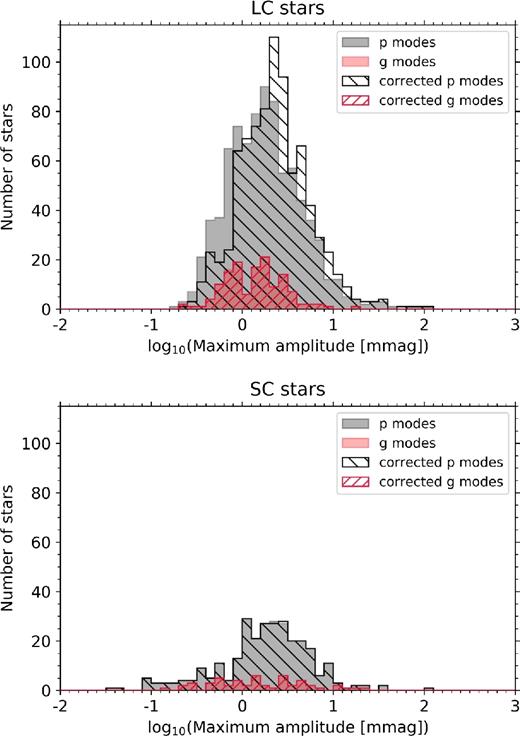
The distributions of the highest amplitude (i.e. dominant) pulsation mode for the ensemble of 963 LC and 334 SC δ Sct stars are shown in the top and bottom panels, respectively. The black and red regions represent the stars for which the dominant pulsation mode is in the p-mode (ν ≥ 4 d−1) or g-mode (ν < 4 d−1) frequency regimes, respectively. The filled regions represent the extracted pulsation mode amplitudes, with the hatched regions of the same colour representing each distribution after being corrected for the amplitude visibility function given in equation (1).
From inspection of Fig. 2, the amplitude of the dominant pulsation mode in a δ Sct star typically lies in between 0.5 and 10 mmag. In each panel, a tail extending from moderate (A ≃ 10 mmag) to high pulsation mode amplitudes (A ≃ 100 mmag) can be seen, which is caused by a small number of HADS stars in each ensemble. Since the SC ensemble contains all δ Sct stars irrespective of the length of data available, coupled with insignificant amplitude suppression described by the amplitude visibility function in equation (1), this demonstrates the intrinsic scarcity of HADS stars in the Kepler data set (Lee et al. 2008; Balona 2016; Bowman 2017).
It is known that the majority of δ Sct stars exhibit amplitude modulation over the 4-yr Kepler data set (Bowman et al. 2016; Bowman 2016), so it could be argued that a different dominant pulsation mode for each δ Sct star could be extracted when using different subsets of Kepler data. However, the amplitude distribution of δ Sct stars would largely remain similar. This can be understood by comparing the top and bottom panels of Fig. 2, calculated using LC and SC Kepler data, respectively. The SC observations of δ Sct stars are randomly distributed throughout the 4-yr Kepler mission, but the distributions in Fig. 2 have similar median and full width at half-maximum values. This demonstrates that the pulsation properties of an ensemble of δ Sct stars are less time-dependent than the pulsation properties of an individual δ Sct star.
4.2 Pulsation and effective temperature
A semi-empirical relationship exists between the effective temperature and the observed pulsation mode frequencies in a δ Sct star, which is caused by the depth of the He ii driving region in the stellar envelope being a function of Teff (Christensen-Dalsgaard 2000; Aerts et al. 2010). A ZAMS δ Sct star near the blue edge of the classical instability strip is expected to pulsate in higher radial overtone modes leading to higher observed pulsation mode frequencies compared to a ZAMS δ Sct star near the red edge of the classical instability strip (Pamyatnykh 1999, 2000; Dupret et al. 2004, 2005). This relationship between effective temperature and pulsation mode frequencies in δ Sct stars has been previously been demonstrated using ground-based observations (see e.g. Breger & Bregman 1975; Breger 2000b; Rodríguez & Breger 2001). Observationally, the blue and red edges are known for ground-based data (Rodríguez & Breger 2001), but the situation becomes less clear when the criterion of S/N ≥ 4 is applied to a data set with a noise level of order a few |$\mu$|mag such as Kepler mission data, as demonstrated in Section 3.
The frequency of the dominant pulsation mode in each δ Sct star in the LC and SC ensembles are shown in the left- and right-hand columns of Fig. 3, respectively. In the top row, the distributions of the dominant pulsation mode frequency are shown by the black region, with the subgroup of stars studied by Tkachenko et al. (2012, 2013) and Niemczura et al. (2015, 2017) shown as the green-hatched region for comparison. Although the LC ensemble suffers from a bias caused by the amplitude visibility function, a dearth of δ Sct stars with pulsation mode frequencies above 60 d−1 exists in both ensembles, such that 0 < ν ≤ 60 d−1 can be considered the typical frequency range of pulsation modes of δ Sct stars in the Kepler data set. These results are not necessarily representative of all δ Sct stars since the TAMS is better sampled compared to the ZAMS in the Kepler data set, with more-evolved δ Sct stars expected to have lower pulsation mode frequencies. The frequency of the dominant pulsation mode does not exceed 60 d−1 in any δ Sct star in either ensemble, which is in agreement with the expectations from theoretical models of MS δ Sct stars near the blue edge of the classical instability strip (Pamyatnykh 1999, 2000).
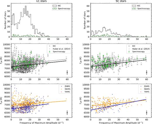
The top row shows the distribution of the frequency of maximum amplitude shown as the black region, with the subgroup of stars studied by Tkachenko et al. (2012, 2013) and Niemczura et al. (2015, 2017) plotted as the green-hatched area. The middle row shows the frequency of maximum amplitude versus the effective temperature, using the KIC, Huber et al. (2014) and spectroscopic values from Tkachenko et al. (2012, 2013) and Niemczura et al. (2015, 2017) as black crosses, grey squares and green circles, respectively, with statistically significant linear regressions shown as solid lines. The bottom row shows the same relationship as the middle row, but for only the KIC stars that have grouped based on their logg value into bins of logg ≥ 4.0 (ZAMS), 3.5 ≤ logg < 4.0 (MAMS), and logg < 3.5 (TAMS). For all rows, the left- and right-hand plots correspond to the LC and SC ensembles, respectively, which have been plotted using the same ordinate and abscissa scales for comparison.
The frequency of the highest amplitude pulsation mode is plotted against Teff for the ensemble of 963 LC and 334 SC δ Sct stars in the middle row of Fig. 3, in which the KIC parameters, the revised Huber et al. (2014) parameters and the subgroup of stars studied by Tkachenko et al. (2012, 2013) and Niemczura et al. (2015, 2017) are shown as black crosses, grey squares, and green circles, respectively. Statistically significant linear regressions are also shown as solid lines, with the gradient, m, intercept, c, coefficient of correlation, R, and p-value obtained from a t-test for each data set given in Table 1. Linear regressions of the frequency of maximum amplitude and effective temperature using either the KIC or Huber et al. (2014) values yield statistically significant positive correlations with R ≃ 0.2 and 0.3 for the LC and SC ensembles, respectively. The amplitude suppression of high-frequency pulsation modes in LC Kepler data explains the weaker correlation between pulsation and effective temperature found in the LC ensemble compared to the SC ensemble, since few δ Sct stars with pulsation mode frequencies above 40 d−1 are included. On the other hand, statistically significant correlations between pulsation and effective temperature for stars in the spectroscopic subgroup were not found. From the relatively large p-values calculated from the linear regression in the spectroscopic subgroup, we cannot claim that the positive correlation found between effective temperature and frequency of the highest amplitude pulsation mode is statistically significant. With few δ Sct stars available with high-resolution spectroscopy, more are needed to investigate this relationship further.
Statistics for linear regressions of the frequency of maximum amplitude and effective temperature for the δ Sct stars in this paper, using KIC values (Brown et al. 2011), the revised KIC values from Huber et al. (2014), and spectroscopic values from Tkachenko et al. (2012, 2013) and Niemczura et al. (2015, 2017). The column headers include the number of stars, Nstars, the gradient, m, the ordinate-axis intercept of the linear fit, c, the coefficient of correlation, R, and the corresponding p-value (obtained from a t-test). Separate regressions for the logg subgroups are given for KIC and Huber et al. (2014) values.
| LC ensemble | SC ensemble | ||||||||||
|---|---|---|---|---|---|---|---|---|---|---|---|
| Nstars | m | c | R | p-value | Nstars | m | c | R | p-value | ||
| (K d−1) | (K) | (K d−1) | (K) | ||||||||
| KIC | |||||||||||
| All | 963 | 12.8 ± 2.0 | 7195 ± 17 | 0.20 | <0.0001 | 334 | 14.1 ± 2.2 | 7229 ± 21 | 0.33 | <0.0001 | |
| ZAMS (logg ≥ 4.0) | 421 | 15.6 ± 3.0 | 6972 ± 16 | 0.24 | <0.0001 | 89 | 22.7 ± 4.0 | 6819 ± 21 | 0.52 | <0.0001 | |
| MAMS (3.5 ≤ logg < 4.0) | 494 | 9.8 ± 2.5 | 7396 ± 17 | 0.17 | 0.0001 | 221 | 11.4 ± 2.5 | 7375 ± 22 | 0.29 | <0.0001 | |
| TAMS (logg < 3.5) | 48 | −7.7 ± 9.9 | 7404 ± 14 | −0.11 | 0.4438 | 24 | 2.3 ± 11.5 | 7442 ± 14 | 0.04 | 0.8460 | |
| Revised KIC | |||||||||||
| All | 963 | 12.1 ± 2.0 | 7424 ± 17 | 0.19 | <0.0001 | 329 | 14.8 ± 2.2 | 7404 ± 21 | 0.34 | <0.0001 | |
| ZAMS (logg ≥ 4.0) | 423 | 15.5 ± 2.9 | 7215 ± 17 | 0.25 | <0.0001 | 85 | 23.0 ± 4.2 | 7027 ± 21 | 0.52 | <0.0001 | |
| MAMS (3.5 ≤ logg < 4.0) | 506 | 9.1 ± 2.6 | 7606 ± 17 | 0.16 | 0.0004 | 224 | 13.1 ± 2.5 | 7512 ± 21 | 0.33 | <0.0001 | |
| TAMS (logg < 3.5) | 34 | −0.5 ± 12.9 | 7525 ± 15 | −0.01 | 0.9710 | 20 | 4.6 ± 12.2 | 7662 ± 17 | 0.09 | 0.7114 | |
| Spectroscopy | |||||||||||
| All | 58 | 11.4 ± 6.7 | 7515 ± 17 | 0.22 | 0.0947 | 70 | 6.2 ± 4.4 | 7625 ± 21 | 0.17 | 0.1584 | |
However, it is important to distinguish that the expectation of hotter δ Sct stars having higher pulsation mode frequencies is predicted for ZAMS stars, with the relationship breaking down for TAMS and post-MS δ Sct stars. As for any star, the frequencies of its pulsation modes decrease, albeit slowly, during the MS because of the increase in stellar radius. This creates a degeneracy when studying an ensemble of stars, with pulsation mode frequencies expected to be correlated with Teff but also correlated with logg (i.e. inversely with age on the MS). In practice, the sensible approach is to test the relationship between the frequency of the dominant pulsation mode and effective temperature for different groups of stars based on their logg value. This is shown in the bottom row of Fig. 3 for stars in the LC and SC ensembles that have grouped into logg ≥ 4.0 (ZAMS), 3.5 ≤ logg < 4.0 (mid-age main sequence; MAMS), and logg < 3.5 (TAMS) using their KIC parameters.
Linear regressions for each of these logg subgroups for the KIC and Huber et al. (2014) values are also included in Table 1, which demonstrate the need to differentiate ZAMS and TAMS stars when studying the pulsational properties of δ Sct stars. For example, as shown in Fig. 3 and given in Table 1, ZAMS stars in the LC and SC ensembles show a statistically significant positive correlation between effective temperature and frequency of the highest amplitude pulsation, with values of R ≃ 0.3 and 0.5, respectively. As discussed previously, the lack of high-frequency pulsators in the LC ensemble explains the difference in these two values. Conversely, no statistically significant correlation was found for TAMS δ Sct stars in either the LC or SC ensembles.
Linear regressions for subgroups based on logg for the δ Sct stars with spectroscopic parameters from Tkachenko et al. (2012, 2013) and Niemczura et al. (2015, 2017) do not provide reliable results because most of these stars have surface gravities between 3.5 ≤ logg ≤ 4.0, and because no significant correlation was found for the subgroup as a whole. Clearly, the ZAMS δ Sct stars, shown in blue in the bottom row of Fig. 3, have the strongest statistical correlation between Teff and frequency of maximum amplitude with R ≃ 0.5, which is in agreement with theoretical models and previous observations (Pamyatnykh 1999, 2000; Breger 2000b; Rodríguez & Breger 2001; Dupret et al. 2004, 2005; Houdek & Dupret 2015).
4.3 Low-frequency variability in δ Sct stars
The incidence of g modes in stars that exceed Teff ≳ 8000 K, especially those with accurate stellar parameters obtained from high-resolution spectroscopy, are interesting cases. These stars are significantly hotter than typical γ Dor stars observed by Kepler, with effective temperatures of γ Dor stars determined using high-resolution spectroscopy typically between 6900 ≤ Teff ≤ 7400 K (Tkachenko et al. 2013; Van Reeth et al. 2015b). The excitation of g modes in δ Sct stars that are located hotter than the blue edge of the γ Dor instability region warrants further study, with such stars found in both LC and SC ensembles. These hot, low-frequency pulsators can be clearly seen in each panel of Fig. 3, in which a non-negligible fraction of stars (originally chosen because they contain only p modes, or p and g modes) have their dominant pulsation mode in the g-mode frequency regime.
A distinct bimodality is present in the top left panel of Fig. 3 with a minimum in the distribution at a frequency of approximately 7 d−1. This minimum in the distribution corresponds to the approximate upper limit of g-mode pulsation frequencies in fast-rotating stars (Bouabid et al. 2013; Van Reeth et al. 2016; Aerts, Van Reeth & Tkachenko 2017b) and an approximate lower limit of p-mode pulsation frequencies, although overlap of g and p modes and their combination frequencies is expected between 4 ≤ ν ≤ 7 d−1. Therefore, the stars with the dominant pulsation mode in the g-mode frequency regime shown in Fig. 3 represent hybrid stars in which the dominant pulsation mode corresponds to a g mode. However, it remains unclear how or why there should be a significant difference, if any, in the respective amplitudes of the p and g modes in a δ Sct star, with all stars in both ensembles selected to contain at least p modes.
The Kepler mission data have proven extremely useful for studying the interior physics of intermediate-mass stars, specifically concerning measurements of radial rotation and angular momentum transport (Aerts et al. 2017b). The first examples of hybrid MS A and F stars with measured interior rotation were by Kurtz et al. (2014) and Saio et al. (2015), and exemplify the power of asteroseismology when applied to hybrid stars such that model-independent measurements of rotation inside stars can be made. To date, a few dozen intermediate-mass MS stars have been found to be almost rigidly rotating or have weak differential rotation (Degroote et al. 2010; Kurtz et al. 2014; Pápics et al. 2014; Saio et al. 2015; Van Reeth et al. 2015a; Triana et al. 2015; Murphy et al. 2016; Ouazzani et al. 2017; Pápics et al. 2017; Zwintz et al. 2017; Van Reeth et al. 2018).
The full asteroseismic potential of studying the hybrid stars using the high-quality Kepler data has yet to be exploited. For example, the observed power excess at low frequencies in γ Dor stars has recently been interpreted as Rossby modes, which further inform our understanding of rotation (Van Reeth et al. 2016; Saio et al. 2018). Furthermore, expanding the systematic search for period spacing patterns beyond the γ Dor stars to the hybrid stars has the prospect of extending the studies of rotation and angular momentum transport to higher masses and fill the gap between the published cases of B and F stars in the literature. The hybrid stars in the LC ensemble have the necessary data quality to extract, identify and model g and p modes which provide valuable physical constraints of the near-core and near-surface regions within a star, respectively, with more observational studies of intermediate- and high-mass stars needed to address the large shortcomings in the theory of angular momentum transport when comparing observations of MS and evolved stars (Tayar & Pinsonneault 2013; Cantiello et al. 2014; Eggenberger et al. 2017; Aerts et al. 2017b).
The study of angular momentum transport in stars has revealed that internal gravity waves (IGWs) stochastically driven in stars with convective cores can explain the observed near-rigid rotation profiles in intermediate-mass stars (Rogers et al. 2013; Rogers 2015). The detection of IGWs can be inferred by the power excess at low frequencies in a star's amplitude spectrum. The few observational detections of IGWs in the literature have been for massive stars of spectral type O, and were made by matching the observed morphology of the low-frequency power excess with that predicted by state-of-the-art simulations of IGWs (Rogers et al. 2013; Rogers 2015; Aerts & Rogers 2015; Aerts et al. 2017a, 2018; Simón-Díaz et al. 2017). Any star with a convective core is predicted to excite IGWs, thus the ensemble of δ Sct stars presented in this work may contain observational signatures of IGWs (e.g. Tkachenko et al. 2014), and warrant further study.
The Kepler data set will remain unchallenged for the foreseeable future for studying δ Sct stars because of its total length, duty cycle, and photometric precision. Furthermore, it represents a homogeneous data set for detections of IGWs and the study of mixing and angular momentum transport in intermediate-mass A and F stars.
4.4 Pulsation within the classical instability strip
The relationships between pulsation mode frequencies and effective temperature and evolutionary stage (i.e. logg) are degenerate, with pulsation mode frequencies predicted and observed to be correlated with both effective temperature and surface gravity. Therefore, using a Teff–logg diagram is a sensible way to investigate these correlations further. The LC and SC ensembles of δ Sct stars are once again plotted in Teff–logg diagrams in the left- and right-hand columns of Fig. 4, respectively, using the KIC parameters for each star. However, unlike the previous diagrams (shown in Fig. 1), each star in Fig. 4 is plotted as a filled circle that has been colour coded by the frequency of its highest amplitude pulsation mode in the top row, and colour coded by the amplitude of its highest amplitude pulsation mode in the bottom row.
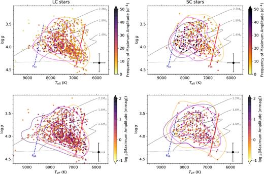
The left- and right-hand columns correspond to the LC and SC ensembles of δ Sct stars, respectively. The top row shows the location of each δ Sct in a Teff–logg diagram using the KIC parameters, with each star's location colour coded by the frequency of the highest amplitude pulsation mode. Similarly, the bottom row is colour coded by the amplitude of the highest amplitude pulsation mode using a logarithmic colour-bar scale. The same stellar evolutionary tracks, ZAMS line, typical KIC error bar, and theoretical edges of the classical instability strip as in Fig. 1 are also shown. In each panel, density contours are plotted for the stars contained within three parts of the shown colour-bar scale.
In each panel in Fig. 4, contour lines corresponding to the 10th, 50th, and 90th percentiles of the normalized probability density after applying a Gaussian kernel to the distribution of stars are shown for three subgroups of stars that fall into three parts of the colour-bar scale. For example, the density maxima in the top right panel of Fig. 4 correspond to approximate Teff values of 7000, 7500, and 8000 K for the 0 < νmax < 20 d−1, 20 ≤ νmax < 40 d−1, and νmax ≥ 40 d−1 subgroups, respectively. Note that since there are so few high-frequency pulsators in the LC ensemble, only two sets of contours are shown in the top left panel of Fig. 4. For the maximum amplitude distributions shown in the bottom row of Fig. 4, the three sets of contours correspond to log10(Amax) ≤ 0, 0 < log10(Amax) < 1 and log10(Amax) ≥ 1. The choice of these subgroups is somewhat arbitrary, but they demonstrate the average trends in each panel and help to guide the eye compared to the distribution using individual stars.
As expected and demonstrated using a subsample of ZAMS stars (logg > 4.0) in Fig. 3, the δ Sct stars with higher pulsation mode frequencies show higher effective temperatures and are found closer to the blue edge of the classical instability strip. The same relationship between effective temperature and pulsation mode frequencies can be seen in the top row of Fig. 4, with high-frequency δ Sct stars (shown in dark purple) being typically located nearer the blue edge of the classical instability strip. The situation is somewhat less clear when studying the relationship between the amplitude of the dominant pulsation mode and location in the Teff − logg, which is shown in the bottom row of Fig. 4. In the LC ensemble, the highest amplitude pulsators (shown in dark purple) are more centrally located in the classical instability strip, whereas the high-amplitude pulsators in the SC ensemble are located closer to the blue edge, but this discrepancy is likely caused by so few high-amplitude stars in each ensemble. It has been previously demonstrated using ground-based observations that HADS stars are often found in the centre of the classical instability strip (McNamara 2000; Breger 2000b), but with so few HADS stars in the Kepler data set and the uncertainties in Teff and logg values, it is difficult to make any meaningful conclusions.
It should be noted that these results may not be completely representative of all δ Sct stars, as only a single pulsation mode frequency was used to characterize each star. This in turn may explain the lack of significant correlation found between the frequency of maximum amplitude, νmax, and effective temperature for all subgroups except ZAMS stars, as described by the results in Table 1. Using space-based observations such as those from Kepler, many δ Sct stars have a large range of pulsation mode frequencies with small amplitudes. The density and range of the observed pulsation mode frequencies are not accounted for when extracting only a single pulsation mode – this is explored in more detail in Section 5. Nonetheless, the high-frequency δ Sct stars are typically located nearer the blue edge of the instability strip as shown in Fig. 4, which is in agreement with theoretical predictions and previous observations of δ Sct stars (Breger & Bregman 1975; Pamyatnykh 1999, 2000; Breger 2000b; Rodríguez & Breger 2001). An interesting result from this analysis is that δ Sct stars across the instability strip are able to pulsate in low and high pulsation mode frequencies, with no obvious explanation for which pulsation modes are excited in δ Sct stars. Further observational and theoretical study of this is needed, as it will provide constrains of mode selection mechanism(s) at work in these stars.
4.5 Pulsation and rotation
The effects of rotation modify the pulsation mode frequencies of a star by lifting the degeneracy of non-radial modes into their 2ℓ + 1 components (Aerts et al. 2010), which are observed as multiplets in a star's amplitude spectrum. The splitting of these component frequencies is significantly asymmetric for moderate and fast-rotating stars, with the Coriolis force acting against the direction of rotation and affects prograde and retrograde pulsation modes differently (Aerts et al. 2010). For a star with numerous non-radial pulsation modes, as is the case for numerous δ Sct stars, the effects of rotation act to increase the observed range of frequencies in an amplitude spectrum (see e.g. Breger et al. 2012). However, there is no expectation for the dominant pulsation mode frequency and/or amplitude of a δ Sct star to be correlated with rotation.
In Fig. 5, the subgroups of LC and SC δ Sct stars that have stellar parameters from Tkachenko et al. (2012, 2013) and Niemczura et al. (2015, 2017) are shown in Teff–logg diagrams in the left- and right-hand panels, respectively. The top row shows the location of each star in a Teff–logg diagram with each star shown as a filled circle colour coded by |$v$| sini determined from spectroscopy. There is no clear correlation amongst effective temperature, surface gravity, and rotation, with slow and fast rotators found across the classical instability strip. Of course, since the spectroscopic values of |$v$| sini are projected surface rotational velocities, they represent lower limits of the true rotation of the stars shown in Fig. 5.
The left- and right-hand columns correspond to the LC and SC ensembles of δ Sct stars, respectively, for which spectroscopic values of Teff, logg, and |$v$| sini are available. The top row shows the location of each δ Sct in a Teff–logg diagram using spectroscopic values from Tkachenko et al. (2012, 2013) and Niemczura et al. (2015, 2017), with each star's location colour coded by |$v$| sini. The same stellar evolutionary tracks, ZAMS line, and theoretical edges of the classical instability strip as in Fig. 1 are also shown in the top row. The bottom row shows the relationship between the frequency and amplitude of the dominant pulsation mode colour coded by |$v$| sini.
In the bottom row of Fig. 5, the relationship between the frequency and amplitude of the dominant pulsation mode is shown, with each star colour coded by |$v$| sini. This figure supports the findings of Breger (2000a) that δ Sct stars with high pulsation mode amplitudes are typically slow rotators (|$v$| sini ≲ 50 km s−1), but clearly not all slowly rotating δ Sct stars have high pulsation mode amplitudes. However, the lack of any significant correlation in the panels of Fig. 5 is not surprising with so few δ Sct stars having been observed with high-resolution spectroscopy.
5 REGULARITIES IN THE AMPLITUDE SPECTRA OF δ S|$\bf ct$| STAR STARS
In this section, a similar methodology as that employed by Michel et al. (2017), who searched for regularities in the amplitude spectra of approximately 1800 δ Sct stars observed by COROT, is applied to the SC ensemble of δ Sct stars presented in this work. It is not informative to perform this analysis using the LC ensemble of δ Sct stars because of the significantly longer integration times of LC Kepler data suppressing high-frequency signals. Consequently, few δ Sct stars exist in the LC ensemble that satisfy the required selection criteria of having high-frequency pulsation modes – i.e. young δ Sct stars. The SC Kepler data were not obtained using as short a cadence as the COROT data, but it is still significantly higher than the pulsation mode frequencies in δ Sct stars.
Following Michel et al. (2017), an amplitude significance criterion was chosen as 10 times the mean amplitude in each star's amplitude spectrum, with the frequency range of νhigh and νlow calculated as the frequency of the highest and lowest amplitude peaks that satisfied the amplitude significance criteria for frequencies above ν ≥ 4 d−1 (|${\gtrsim } 50 \, \mu$|Hz). This minimum in frequency is approximately twice the value chosen by Michel et al. (2017), but we use 4 d−1 in this study to reduce the chance that the extracted values of νlow represent g-mode pulsation frequencies. Each star's amplitude spectrum was interpolated on to a frequency resolution of 0.05 d−1 using the maximum amplitude value of each bin in the original spectrum. This downgrades each amplitude spectrum to the approximate Rayleigh resolution criterion for a data set of approximately 20 d in length, but preserves the amplitude content from the original high-resolution and oversampled Fourier transform. This step is necessary to produce a figure with structure that can be resolved by the human eye. Also, it has the added advantage of homogenizing the amplitude spectra in the SC ensemble irrespective of data set length. The modified amplitude spectra, shown between 0 < ν < 90 d−1, are stacked in order of increasing effective temperature using KIC values and are shown in Fig. 6. In this figure, solid red lines are used to indicate a moving average of the observables νlow and νhigh along the star number ordinate axis. The stacked amplitude spectra show an increase in the frequencies of pulsation modes for increasing Teff, but also show an increase in the range of observed pulsation mode frequencies for hotter δ Sct stars. Therefore, not only does the frequency of maximum amplitude, νmax, increase with increasing Teff, but so do the observables νlow and νhigh.
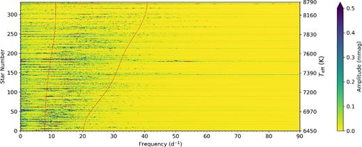
The stacked amplitude spectra for the ensemble of SC δ Sct stars in order of increasing Teff using KIC values in an upwards direction, with the red lines indicating a moving average of the νlow and νhigh values along the star number ordinate axis. Indicative effective temperature values are also included on the ordinate axis to demonstrate how νlow and νhigh vary with Teff.
The distribution of the νhigh and νlow values for each star in the SC ensemble is shown in Fig. 7, with each star shown as a filled circle colour coded by the amplitude of the dominant pulsation mode. Using the same criteria as Michel et al. (2017), a subsample of young δ Sct stars was created by including the δ Sct stars with νhigh ≥ 35 d−1 (|${\gtrsim } 400 \, \mu$|Hz) and the ratio of the highest and lowest frequencies in each star satisfying (νhigh/νlow) < 4.5. These selection criteria are shown graphically by the individual solid black lines in Fig. 7, with the enclosed grey region indicating the subsample of young δ Sct stars. This subgroup contains 60 δ Sct stars, which is noticeably fewer than the ∼250 COROT stars presented by Michel et al. (2017). To include more young stars using the SC Kepler data, the νhigh restriction would have to be relaxed substantially below 35 d−1, but this boundary is motivated by theoretical models of pulsation mode frequencies in young δ Sct stars being above 35 d−1 and changing this criterion removes the compatibility with the analysis by Michel et al. (2017).
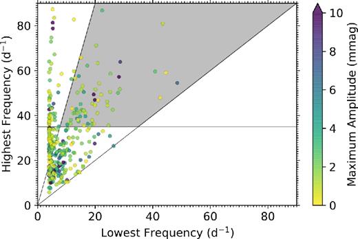
The distribution of lowest and highest frequencies of peaks with amplitudes greater than 10 times the mean amplitude in the amplitude spectrum above ν ≥ 4 d−1 for the ensemble of SC δ Sct stars. Each star has been colour coded by the amplitude of the highest amplitude peak in the amplitude spectrum and the grey region denotes the subsample of young δ Sct stars based on νhigh > 35 d−1 and a ratio of (νhigh/νlow) < 4.5. Since νlow and νhigh are extracted in the frequency range of 4 ≤ ν ≤ 98 d−1, they can be significantly smaller or larger than the corresponding νmax value for each star (cf. Section 4).
The stacked amplitude spectra of this subgroup of young δ Sct stars using SC Kepler data are plotted in the top panel of Fig. 8 in order of ascending values of νhigh. The high-frequency ridges observed in the amplitude spectra of young δ Sct stars studied by Michel et al. (2017) were shown to be consistent with axisymmetric island modes using theoretical models of fast-rotating stars (Reese et al. 2009). To examine any similar ridges in the amplitude spectra using SC Kepler data, the amplitude spectra were normalized by νhigh and are plotted on a logarithmic frequency scale in the bottom panel of Fig. 8, in which the rows above the white space show an average amplitude spectrum for the 60 δ Sct stars in the panel. The ridges and regularities discussed by Michel et al. (2017) are evident in a fraction, but not all, of the amplitude spectra shown in Fig. 8. Furthermore, the ridge-like structure is not always near the value of νhigh in a star's amplitude spectrum. For example, the last star in the top panel of Fig. 8 has several ridges separated by approximately 3 d−1 in its amplitude spectrum between 35 ≤ ν ≤ 45 d−1, which could correspond to the large-frequency separation in this star, but the value of νhigh ≃ 80 d−1 using the S/N ≥ 10 amplitude criterion described previously clearly corresponds to higher frequencies that are harmonics and combination frequencies of these ridges and not intrinsic pulsation modes.
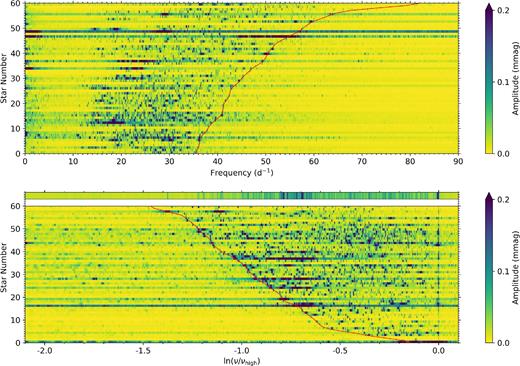
The top panel shows the subsample of young δ Sct stars from the SC ensemble, which were chosen as the stars that satisfied νhigh > 35 d−1 and a ratio of (νhigh/νlow) < 4.5 similar to Michel et al. (2017). The solid red line indicates a moving average of the νhigh values along the star number ordinate axis. The bottom panel is the same subgroup of stars as the top panel, but with each star's amplitude spectrum having been normalized by its νhigh value and shown on a logarithmic abscissa scale. The solid red line indicates a moving average of the νlow values along the star number ordinate axis. In the bottom panel, the three rows above the white space show an average of the 60 normalized amplitude spectra. The colour scale in both panels has been purposefully chosen to have an upper limit of 0.2 mmag to reveal low-amplitude peaks, which is similar to the arbitrary upper value of 0.2 parts per thousand (ppt) chosen by Michel et al. (2017).
Other stars similarly have ridges in their amplitude spectra that do not appear near their νhigh values, which explains the lack of regularity in the average amplitude spectrum shown in the rows above the white space in the bottom panel in Fig. 8. Therefore, this method of normalizing amplitude spectrum by νhigh is strongly dependent on the selection criteria used in determining νhigh and is not consistent for all stars. This is easily understood since all peaks in a star's amplitude spectra above S/N ≥ 10 in amplitude were included in the determination of νlow and νhigh. However, it is possible for a δ Sct star to have harmonics and combination frequencies that have amplitudes larger than the chosen amplitude criterion, so a larger νhigh value can be used for such a star which corresponds to a harmonic or a combination frequency rather than a pulsation mode frequency.
The frequency spacing between consecutive radial order p modes in a δ Sct star is of order a few d−1, but the specific value depends on the stellar parameters and the radial orders of the pulsation modes (Breger, Lenz & Pamyatnykh 2009; García Hernández et al. 2015; Van Reeth et al. 2018). Furthermore, although p modes in δ Sct stars are typically low radial order, pulsation modes of higher radial order can be considered in the transition region where the asymptotic relation for p modes applies, such that p modes are equally spaced in frequency. The mode-dependent transition in the validity of the asymptotic relation for p modes would break the expectation of finding equally spaced ridges in the logarithmic plot shown in the bottom panel of Fig. 8, but the amplitude spectra in linear unnormalized frequencies would remain unaffected for high radial orders. This is certainly true for the stars in Fig. 1 that lie hotter than the blue edge of the classical instability strip and are inferred to be pulsating in p modes with radial orders of n ≥ 6.
Therefore, the stars identified as young δ Sct stars in Fig. 8, which were selected because they have high pulsation mode frequencies (νhigh ≥ 35 d−1) corresponding to young stars and inferred to be close to the ZAMS based on predictions from theoretical models (Michel et al. 2017), represent a subgroup of δ Sct stars for which mode identification is simplified because of the presence of regularities in their amplitude spectra. Further observational and theoretical study for the stars showing regularities in their amplitude spectra is required, as they provide insight of mode excitation and interior physics such as rotation and mixing in δ Sct stars where mode identification is possible, cf. Van Reeth et al. (2018).
6 DISCUSSION AND CONCLUSIONS
Two ensembles of δ Sct stars using LC and SC Kepler data consisting of 963 and 334 stars, respectively, were compiled and used to characterize the ensemble pulsational properties of intermediate-mass A and F stars. The LC Kepler sampling frequency of 48.9 d−1 introduces a bias towards extracting low-frequency pulsation modes in an iterative pre-whitening procedure, with higher frequencies being suppressed in amplitude. The amplitude visibility function given in equation (1) explains the dearth of δ Sct stars with pulsation mode frequencies above ν ≥ 40 d−1 in LC Kepler data. The amplitude visibility function is negligible in the SC ensemble since the SC sampling frequency is 1476.9 d−1; the limitation of these data is that fewer δ Sct stars were observed in SC than in LC, and typically not for time spans longer than 30 d which has a poor frequency resolution in comparison.
The distributions of δ Sct stars in Teff–logg diagrams shown in Fig. 1 demonstrate that the theoretical edges of the classical instability strip for modes of radial orders between 1 ≤ n ≤ 6 calculated by Dupret et al. (2005) are mostly consistent with observations of δ Sct stars from the Kepler Space Telescope. However, a minority of δ Sct stars, including some with stellar parameters obtained using high-resolution spectroscopy by Tkachenko et al. (2012, 2013) and Niemczura et al. (2015, 2017), are hotter than the blue edge and/or cooler than the red edge of the classical instability strip depending on the source of stellar parameters (e.g. Brown et al. 2011; Huber et al. 2014). Furthermore, the boundaries of the classical instability strip calculated by Dupret et al. (2005) were calibrated using ground observations of δ Sct stars, which typically have high levels of noise in their amplitude spectra, thus are limited to high pulsation mode amplitudes. The analysis of a large number of δ Sct stars in this work supports the requirement for a mass-dependent value of the αMLT parameter in theoretical models to reproduce all δ Sct stars in a Teff–logg diagram. This is particularly necessary to explain the hot δ Sct stars that are beyond the blue edge of the n = 6 radial mode using αMLT = 1.8 (Dupret et al. 2004, 2005).
The distributions of maximum pulsation amplitude for the LC and SC ensembles were shown to be consistent with each other, as shown in Fig. 2, with typical dominant pulsation mode amplitudes between 0.5 and 10 mmag found for most δ Sct stars. Similar high-amplitude tails in the amplitude distributions of the LC and SC data are also evident, which are caused by the presence of HADS stars in the Kepler mission data. These stars have been previously demonstrated to be rare (Lee et al. 2008; Balona 2016; Bowman 2017), a finding that is supported by the scarcity of these stars in both LC and SC ensembles in this work. It remains unclear if HADS stars are physically distinct from their low-amplitude counterparts (Breger 2000b; Balona 2016; Bowman 2016, 2017). Further work is needed to address this.
Despite the lack of amplitude suppression, few δ Sct stars exist in the Kepler data set with pulsation mode frequencies above 60 d−1, with no δ Sct stars having their dominant pulsation mode above 60 d−1 as shown in Fig. 3. This is in agreement with previous analyses of δ Sct stars using subsets of Kepler data (Balona & Dziembowski 2011) if such studies had been corrected for the amplitude visibility function (equation 1). The dearth of high-frequency δ Sct stars observed by Kepler can be explained by the lack of hot ZAMS stars, with the TAMS being better sampled in comparison (Tkachenko et al. 2012, 2013; Niemczura et al. 2015, 2017). The correlations between the pulsation mode frequencies, effective temperature, and evolutionary stage (logg by proxy) were investigated and shown in Fig. 3. The ensembles were separated into ZAMS (logg ≥ 4.0), MAMS (3.5 ≤ logg < 4.0), and TAMS (logg < 3.5) subgroups using the KIC values, with separate linear regressions between the frequency of the highest amplitude pulsation mode and Teff for each logg subgroup demonstrating a stronger correlation for ZAMS stars in the SC data. For a ZAMS δ Sct star near the blue edge of the classical instability strip, a high effective temperature facilitates the excitation of higher overtone p modes and higher observed pulsation mode frequencies because the κ mechanism operating in the He ii ionization zone is closer to the surface of the star (Pamyatnykh 1999, 2000; Dupret et al. 2004, 2005). This relationship was also found in ground-based observations of δ Sct stars (Breger & Bregman 1975; Breger 2000b; Rodríguez & Breger 2001).
Following a similar methodology to that employed by Michel et al. (2017) who classified and studied approximately 250 young δ Sct stars observed by COROT, regularities were searched for in the amplitude spectra of 60 young δ Sct stars identified in the SC ensemble of Kepler observations using the same requirement of high-frequency (ν ≥ 35 d−1) pulsation modes in their amplitude spectra. Similar ridges consistent with consecutive radial order p modes can be seen at high frequency in the amplitude spectra of some, but not all, of these young δ Sct stars in the SC ensemble. This can partially be explained by the amplitude significance criterion used to determine the observables νlow and νhigh, specifically how harmonics and combination frequencies need to be identified when searching for the frequency separation between radial order p modes. However, a fraction of the stars shown in Fig. 8 do show frequency ridges with spacings of order a few d−1, which are consistent with axisymmetric island modes predicted by theoretical models of fast-rotating stars (Reese et al. 2009; Michel et al. 2017).
The lack of a complete theory for pulsation mode excitation, specifically the non-linear effects that determine the amplitudes of pulsation modes, means we are unable to realistically predict the amplitudes of pulsation modes using current theoretical models. To test if one expects significant regularities caused by the separation between consecutive radial modes in the amplitude spectra of δ Sct stars, Reese et al. (2017) investigated multiplying the intrinsic amplitudes from theoretical amplitude spectra by random numbers uniformly drawn from between 1 and 100 on a logarithmic scale. This proxy for a non-linear mode saturation mechanism, combined with fast rotation, pulsation mode visibility, and observing a star at an unknown inclination angle led Reese et al. (2017) to conclude that finding such regularities in δ Sct stars is unlikely. The exceptions to this were found in so-called favourable scenarios where 2Ω coincided with Δν or Δν/2 corresponding to 30 and 70 per cent of the break-up velocity (Reese et al. 2017). The lack of significant regularities in the majority of the amplitude spectra of young δ Sct stars presented in this work is consistent with the conclusions presented by Reese et al. (2017). On the other, those δ Sct stars with regularities consistent with consecutive radial order p modes may provide valuable constraints of rotation and inclination of δ Sct stars based on the discussion by Reese et al. (2017), which are typically difficult parameters to determine for δ Sct stars.
Other added complications when studying the amplitude spectra of δ Sct stars are non-linearity in the form of mode coupling between pulsation modes, and non-linearity in the form of harmonics and combination frequencies (Breger & Montgomery 2014; Bowman 2017), which create pseudo-regularities and dense forest-like amplitude spectra. It is also important to note that the pulsation modes in δ Sct stars can potentially cover a large range of radial orders such that the expected frequency separation between consecutive radial order p modes in a star is not a constant. This can be understood from the transition from moderate to high values of n coinciding with the transition for which the asymptotic approximation applies. This produces a non-constant value for the frequency separation across several radial orders in δ Sct stars further complicating the task of finding regularity in a star's amplitude spectrum (see e.g. Breger et al. 2009). All the discussed effects act towards blurring the mean of the normalized amplitude spectrum for an ensemble of δ Sct stars, which explains the lack of regularity in the average amplitude spectrum shown in the rows above the white space in the bottom panel of Fig. 8.
Many δ Sct stars are observed to have low-frequency peaks in their amplitude spectra (Balona 2014; Balona et al. 2015), which can be identified as combination frequencies or independent g-mode pulsations (see e.g. Saio et al. 2018). The full scientific potential of these hybrid stars is yet to be established, with direct measurements of rotation and angular momentum transport needed in A stars to fill the gap between B and F stars and constrain theoretical models (Van Reeth et al. 2016; Aerts et al. 2017b). Asteroseismic modelling of the most-promising δ Sct stars, for which mode identification is possible, using the stellar evolution code mesa (Paxton et al. 2011, 2013, 2015) and the pulsation code gyre (Townsend & Teitler 2013), will constrain theoretical models of interior physics in these stars (see e.g. Van Reeth et al. 2018). The ensemble of 963 δ Sct stars observed continuously by the Kepler Space Telescope with an unprecedented photometric precision is currently the best data set for studying the interior physics of A stars and will remain of great use for many years to come.
Acknowledgements
DMB would like to thank the Kepler science team for providing such excellent data, and Prof Conny Aerts, Dr Péter Pápics, and Dr Timothy Van Reeth for useful discussions. Funding for the Kepler mission is provided by NASA's Science Mission Directorate. The Kepler data presented in this paper were obtained from the MAST. Support for MAST for non-HST data is provided by the NASA Office of Space Science via grant NNX09AF08G and by other grants and contracts. The research leading to these results has received funding from the European Research Council under the European Union's Horizon 2020 research and innovation programme (grant agreement number 670519: MAMSIE). This research has made use of the SIMBAD data base, operated at CDS, Strasbourg, France; the SAO/NASA Astrophysics Data System; and the VizieR catalogue access tool, CDS, Strasbourg, France. We thank the referee for their comments that improved the manuscript.
Footnotes
MAST website: http://archive.stsci.edu/kepler/.
an updated list of known Kepler eclipsing binary stars can be found at: http://keplerebs.villanova.edu.
Kepler data release notes: https://archive.stsci.edu/kepler/data_release.html.
Examples of mono-periodic δ Sct stars include KIC 5989856, KIC 8196006, KIC 8196381, and KIC 11509728, which were identified by Bowman et al. (2016) as having only a single significant pulsation mode in the p-mode frequency range.
REFERENCES
