


Abstract
Two sets of rate coefficients for low-energy inelastic potassium-hydrogen and rubidium-hydrogen collisions were computed for each collisional system based on two model electronic structure calculations, performed by the quantum asymptotic semi-empirical and the quantum asymptotic linear combinations of atomic orbitals (LCAO) approaches, followed by quantum multichannel calculations for the non-adiabatic nuclear dynamics. The rate coefficients for the charge transfer (mutual neutralization, ion-pair formation), excitation and de-excitation processes are calculated for all transitions between the five lowest lying covalent states and the ionic states for each collisional system for the temperature range 1000–10 000 K. The processes involving higher lying states have extremely low rate coefficients and, hence, are neglected. The two model calculations both single out the same partial processes as having large and moderate rate coefficients. The largest rate coefficients correspond to the mutual neutralization processes into the K(5s 2S) and Rb(4d 2D) final states and at temperature 6000 K have values exceeding 3 × 10⁻⁸ cm3 s−1 and 4 × 10⁻⁸ cm3 s−1, respectively. It is shown that both the semi-empirical and the LCAO approaches perform equally well on average and that both sets of atomic data have roughly the same accuracy. The processes with large and moderate rate coefficients are likely to be important for non-LTE modelling in atmospheres of F, G and K-stars, especially metal-poor stars.
1 INTRODUCTION
The lack of data on inelastic processes due to collisions with neutral hydrogen atoms has been a major limitation on modelling of F-, G- and K-star spectra in statistical equilibrium, and thus to reliably proceeding beyond the assumption of local thermodynamic equilibrium (LTE) in analysis of stellar spectra and the determination of elemental abundances. This problem has been well documented, e.g. see Lambert (1993); Barklem (2016a) and references therein. Significant progress has been made in recent times through detailed full-quantum scattering calculations, based on quantum chemical data, for the cases of simple atoms such as Li, Na, Mg and Ca (Belyaev & Barklem 2003; Barklem, Belyaev & Asplund 2003; Belyaev et al. 2010; Barklem et al. 2010; Belyaev et al. 2012; Barklem et al. 2012; Mitrushchenkov et al. 2017). These calculations have demonstrated the importance of the ionic-covalent curve crossing mechanism leading naturally to charge transfer processes (mutual neutralization and ion-pair production), in addition to excitation and de-excitation processes. The importance of this mechanism has allowed various simplified model approaches to be developed, which may be used in cases where suitable quantum chemistry data are not been available. In particular a semi-empirical model has been employed for Al, Si, Be and Ca (Belyaev 2013a,b; Belyaev, Yakovleva & Barklem 2014b; Yakovleva, Voronov & Belyaev 2016; Belyaev et al. 2016), and a theoretical model based on a two-electron asymptotic linear combinations of atomic orbitals (LCAO) approach, has also been employed for Ca (Barklem 2016b, 2017). Comparisons of the two methods show quite good agreement and reasonable agreement with the full quantum calculations is found, particularly for the most important processes with the largest rates (Barklem 2016b, 2017; Mashonkina, Sitnova & Belyaev 2017; Mitrushchenkov et al. 2017). Thus, the model approaches provide a useful route for obtaining estimates of the rates for these processes for many elements of astrophysical interest.
In this work, data for the remaining alkalis of astrophysical interest, K and Rb, are calculated using the two model approaches. The use of the two methods, and two independent codes, provides a useful check on the calculations and a means to estimate the sensitivity of the calculations to the underlying methods and assumptions. We note the case of the remaining alkali Cs has been studied theoretically (Belyaev, Lepetit & Gadéa 2014a), but is not observed in stars. Due to their low abundance and low ionization potential, K and Rb have only a small number of lines observable in the visual and infrared spectrum, due to the neutral species, and these features are often blended. However, recent years have seen an increase in interest in these elements, particularly in globular cluster stars, due to discovered anticorrelations of K with Mg abundances (Cohen & Kirby 2012; Mucciarelli et al. 2012, 2015; Iliadis et al. 2016; Mucciarelli, Merle & Bellazzini 2017), and the use of Rb as an important diagnostic of the nature of the s-process (Yong et al. 2006; D'Orazi1 et al. 2013; Yong et al. 2014). Numerous statistical equilibrium calculations have been performed for K (Shchukina 1987; Bruls, Rutten & Shchukina 1992; Takeda et al. 1996; Ivanova & Shimanskiĭ 2000; Takeda et al. 2002; Zhang et al. 2006a,b; Scott et al. 2015), often with hydrogen collisions included using a scaling of the Drawin formula (Steenbock & Holweger 1984). The data provided here allow such approximate recipes with free parameters to be avoided. To our knowledge, no such statistical equilibrium calculations have been attempted for Rb, but the data provided here gives the possibility to attempt such calculations in future. An additional reason to treat collisions of hydrogen with alkalis is that mutual neutralization cross-sections in these collisions may be accessible to experiment, in particular with DESIREE (Thomas et al. 2011).
2 MODEL APPROACHES, GENERAL REMARKS
This study of inelastic processes in potassium-hydrogen and rubidium-hydrogen collisions is performed within the framework of the Born–Oppenheimer formalism, which is the most widely used and reliable approach for theoretical studies of low-energy heavy-particle collisions. The approach treats the collision problem in two steps: a fixed-nuclei electronic structure calculation and a non-adiabatic nuclear dynamical study. Full quantum calculations in both steps are time-consuming. For this reason the present calculations are accomplished by means of quantum model approaches for both steps.
As mentioned in the introduction, the main mechanism for inelastic collision processes with large and moderate rate coefficients arises from ionic-covalent interactions, for which long-range adiabatic potentials may first and foremost be estimated using two asymptotic quantum model approaches: the asymptotic semi-empirical approach (Olson, Smith & Bauer 1971; Belyaev 2013a); and the asymptotic LCAO method (Grice & Herschbach 1974; Adelman & Herschbach 1977; Barklem 2016b, 2017). These two approaches have some features in common, but also some differences. Both model approaches calculate first the electronic Hamiltonian matrix in the form of an arrow matrix, that is, the diagonal matrix elements in a diabatic representation (diabatic potentials correlated to corresponding atomic energies) and asymptotic off-diagonal exchange matrix elements due to the ionic-covalent interaction (covalent–covalent off-diagonal matrix elements are omitted). Diagonalization of the Hamiltonian matrix constructed in this way provides adiabatic potentials needed for the non-adiabatic nuclear dynamics. The key point in the electronic structure calculation is the calculation of the exchange ionic-covalent matrix elements. This is done in different ways in the semi-empirical and the LCAO approaches. The asymptotic semi-empirical approach (Belyaev 2013a) is based on the semi-empirical formula proposed by Olson et al. (1971) for a long-range exchange ionic-covalent matrix element averaged over electronic angular momentum quantum numbers, while the asymptotic LCAO method (Barklem 2016b) calculates these matrix elements based on unperturbed atomic orbital wave functions and takes electronic angular momentum addition into account explicitly. The ways for evaluating diagonal matrix elements are also slightly different: the semi-empirical approach takes the analytical form for the long-range diabatic potentials, while the LCAO method simply adopts atomic energies. The fine structure is neglected. Comparisons of CaH adiabatic potentials in the avoided crossing non-adiabatic regions computed by the semi-empirical (Belyaev et al. 2016) and by the LCAO (Barklem 2016b, 2017) approaches with ab initio potentials (Mitrushchenkov et al. 2017) show that the semi-empirical and the LCAO models perform roughly equally well on average.
For the second step, the non-adiabatic nuclear dynamics, two quantum model approaches have been proposed for estimating state-to-state non-adiabatic transition probabilities: (i) the branching probability current method (Belyaev 2013a); and (ii) the multichannel model approach (Belyaev & Tserkovnyi 1987; Belyaev 1993; Belyaev & Barklem 2003; Belyaev et al. 2014b; Yakovleva et al. 2016). Both approaches are based on the Landau–Zener model for non-adiabatic transitions and take into account the presence of multiple non-adiabatic regions. In addition to long-range regions, the former approach takes into account also short-range ones, but the latter is advantageous because it is analytical. It requires a system to pass non-adiabatic regions in a particular order (see e.g. Yakovleva et al. 2016) and this is the case for avoided crossings formed by the ionic-covalent interaction. Thus, the quantum multichannel approach is applied in this work for calculating state-to-state inelastic transition probabilities. Short-range non-adiabatic regions are currently neglected, as it has been proven by both full quantum (Belyaev et al. 2012) and model (Belyaev 2013a; Mitrushchenkov et al. 2017) calculations that this is a good approximation for computing large-valued rate coefficients. The inelastic cross-sections and rate coefficients are then computed as usual.
As mentioned in the introduction, comparison with available full quantum results has shown that the model approaches provide reliable collision data (Belyaev et al. 2014b; Barklem 2016b), especially for processes with large and moderate rate coefficients, such processes being the most important for non-LTE modelling (see e.g. Barklem et al. 2003; Lind et al. 2011; Barklem 2016a; Osorio & Barklem 2016). Thus, this study of inelastic processes in low-energy potassium-hydrogen and rubidium-hydrogen collisions is accomplished as follows. The electronic structure calculations are performed by means of both the quantum model semi-empirical approach and the quantum model LCAO approach. The non-adiabatic nuclear dynamical calculations are carried out by means of the multichannel model approach for each set of non-adiabatic parameters obtained from the electronic structure calculations by means of two independent dynamical codes. Very recently, Markson & Sadeghpour (2016) have developed a model approach that could be applied to systems such as those studied here, and future comparisons would be of interest.
3 POTASSIUM-HYDROGEN COLLISIONS
3.1 Electronic structure
The scattering channels treated in this study of inelastic collisions K+ + H− and K(nl) + H are listed in Table 1. Since large and moderate rate coefficients correspond to non-adiabatic transitions due to the ionic-covalent interaction, the molecular symmetry of the ground ionic molecular state should be considered. This ground ionic molecular state has 1Σ+ symmetry, and for this reason only the scattering channels of this molecular symmetry are taken into account. Molecular states of other symmetries are not included in the present consideration.
KH(j1Σ+) collisional channels and asymptotic energies with respect to the ground state. The asymptotic energies of the scattering channels coincide with the corresponding electronic energy levels of the atom, which are adopted as J-averaged experimental values taken from NIST (Kramida, Ralchenko & Reader 2016).
| Scattering | Asymptotic | |
|---|---|---|
| j | channels | energies (eV) |
| 1 | K(4s 2S) + H(1s2S) | 0.000 |
| 2 | K(4p 2P) + H(1s2S) | 1.615 |
| 3 | K(5s 2S) + H(1s2S) | 2.607 |
| 4 | K(3d 2D) + H(1s2S) | 2.670 |
| 5 | K(5p 2P) + H(1s2S) | 3.064 |
| i | K+(1S) + H−(1s21S) | 3.586 |
| Scattering | Asymptotic | |
|---|---|---|
| j | channels | energies (eV) |
| 1 | K(4s 2S) + H(1s2S) | 0.000 |
| 2 | K(4p 2P) + H(1s2S) | 1.615 |
| 3 | K(5s 2S) + H(1s2S) | 2.607 |
| 4 | K(3d 2D) + H(1s2S) | 2.670 |
| 5 | K(5p 2P) + H(1s2S) | 3.064 |
| i | K+(1S) + H−(1s21S) | 3.586 |
It is seen from Table 1 that only five atomic states of K are included from the ground and up to K(5p). Other higher lying atomic states create covalent molecular KH states, which either produce non-adiabatic regions at large internuclear distances (three atomic states, K(4d), K(6s), K(4f), at distances larger than 100 atomic units ≡ a.u.) or do not produce avoided crossings at all. For this reason, corresponding rate coefficients from/into these higher lying states are likely to be negligibly small, and these states are neglected.
As described in the previous section, in order to calculate avoided crossings, which are responsible for inelastic transitions leading to large and moderate rate coefficients, two model approaches have been used in this work: the semi-empirical and the LCAO ones. Fig. 1 shows the results the calculations of these non-adiabatic regions by means of the semi-empirical model approach, as well as by the LCAO ones. Short-range potentials estimated by these approaches are not shown because only the long-range non-adiabatic regions determine essentially the low-energy collision rate coefficients with large and moderate values. A series of avoided crossings due to the ionic-covalent interactions is clearly seen. In each avoided crossing non-adiabatic region, the Landau–Zener parameter is calculated by means of the adiabatic-potential-based formula (Belyaev & Lebedev 2011), which allows one to compute the non-adiabatic transition probability. The comparison of the calculated potentials with the accurate pseudo-potential KH data (Khelifi, Oujia & Gadea 2002b) shows a good qualitative agreement. Unfortunately, there is no possibility to make a quantitative comparison, as the numerical data for the pseudo-potential results are not available. Other calculations, see e.g. Geum et al. (2001), were not performed for excited states and this prevents using them for non-adiabatic transitions.
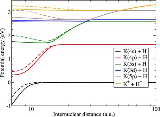
The KH(1Σ+) adiabatic potential energy curves obtained by means of the model semi-empirical approach (solid curves) and by the model LCAO approach (dashed curves).
Since the non-adiabatic (avoided crossing) regions are located in a particular order, the multichannel approach is applicable. As described above, a non-adiabatic transition probability in each non-adiabatic region is calculated by means of the Landau–Zener model. The multichannel analytic formulae (Yakovleva et al. 2016) are then used for computing the inelastic probability for each state-to-state transition. Finally, the inelastic cross-sections and rate coefficients are calculated for all transitions between the scattering channels collected in Table 1.
3.2 Non-adiabatic nuclear dynamics
Rate coefficients Kif(T) for the excitation, de-excitation, mutual neutralization and ion-pair formation processes in potassium-hydrogen collisions are calculated in this work and published online as supplementary material1 to this paper for the temperature range T = 1000–10 000 K. For the temperature T = 6000 K these rate coefficients are presented in Table 2. The value in the upper position in each cell of the table corresponds to the rate coefficient computed based on the adiabatic potentials obtained from the model semi-empirical approach, while the value in the lower position corresponds to the LCAO one. Since the non-adiabatic dynamical treatment in both calculations is essentially the same, the differences come from the electronic structure calculations. Fig. 2 shows the same rate coefficients in the form of graphical representation.
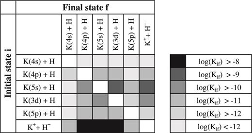
Graphical representation of the rate coefficients Kif(T) (in units of cm3 s−1) for the inelastic processes in K + H and K+ + H− collisions at temperature T = 6000 K calculated by means of the semi-empirical approach.
Rate coefficients, in units of cm3 s−1, at T = 6000 K for the excitation, de-excitation, ion-pair formation and mutual neutralization processes in potassium-hydrogen collisions. For each initial state the value on the upper line corresponds to the model semi-empirical approach calculations, while the lower line corresponds to the LCAO calculations.
| Initial | Final state | |||||
|---|---|---|---|---|---|---|
| state | K(4s) +H | K(4p) +H | K(5s) +H | K(3d) +H | K(5p) +H | K+ + H− |
| K(4s) +H | – | 1.59E-13 | 2.85E-15 | 1.67E-15 | 6.77E-17 | 8.26E-15 |
| – | 6.30E-14 | 2.01E-16 | 1.40E-16 | 8.14E-18 | 1.84E-15 | |
| K(4p) +H | 1.20E-12 | – | 2.48E-11 | 1.40E-11 | 8.07E-13 | 3.00E-11 |
| 4.73E-13 | – | 3.14E-12 | 1.89E-12 | 3.39E-13 | 1.16E-11 | |
| K(5s) +H | 4.42E-13 | 5.07E-10 | – | 1.17E-09 | 6.30E-11 | 1.22E-09 |
| 3.13E-14 | 6.49E-11 | – | 8.07E-10 | 2.73E-10 | 1.30E-09 | |
| K(3d) +H | 5.83E-14 | 6.46E-11 | 2.64E-10 | – | 9.90E-12 | 1.89E-10 |
| 4.92E-15 | 8.82E-12 | 1.82E-10 | – | 5.71E-11 | 2.56E-10 | |
| K(5p) +H | 8.45E-15 | 1.33E-11 | 5.08E-11 | 3.54E-11 | – | 1.39E-12 |
| 1.02E-15 | 5.64E-12 | 2.20E-10 | 2.03E-10 | – | 5.62E-12 | |
| K+ + H− | 3.40E-11 | 1.63E-08 | 3.23E-08 | 2.22E-08 | 4.58E-11 | – |
| 7.59E-12 | 6.39E-09 | 3.47E-08 | 3.02E-08 | 1.87E-10 | – | |
It is seen from Table 2 and Fig. 2 that the largest rate coefficients correspond to the mutual neutralization processes. Fig. 3 plots the rate coefficients for these processes. It is seen from Table 2 and Fig. 3 that in both calculations the largest rate coefficient corresponds to the transition into the K(5s), that is, to the process K+ + H− → K(5s) + H. The corresponding rate coefficient exceeds 3.2 × 10⁻⁸ cm3 s−1. The deviation between the two calculations is below 10 per cent.
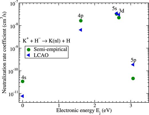
Rate coefficients for the mutual neutralization processes K+ + H− → K(nl) + H at temperature T = 6000 K calculated by means of the model asymptotic semi-empirical approach (circles) and the asymptotic LCAO approach (triangles). The final states are shown at the corresponding electronic energies Ej of the potassium atom, see Table 1.
The next largest rate coefficient corresponds to the mutual neutralization process into K(3d): K+ + H− → K(3d) + H. The corresponding rate coefficient exceeds 2 × 10⁻⁸ cm3s−1, and the deviation is below 30 per cent in this case. Mutual neutralization into the K(4p) state also has a large value though a larger deviation. The neutralization into the K(4s) and K(5p) states have much smaller values and deviations are within a factor of 5.
Amongst the (de-)excitation, the largest rate coefficients correspond to the processes from the K(5s) state, that is, the following processes: K(5s) + H → K(nl) + H. The rate coefficients for these processes are plotted in Fig. 4. It is seen that the largest rate corresponds to the 5s → 3d transition, and that this rate coefficient is around 10−9cm3 s−1, that is, more 30 times smaller than the largest neutralization rate coefficient. The deviation between the rates calculated by the different model approaches for this partial process is approximately 30 per cent. For other partial (de-)excitation processes deviations are larger, but the rates agree with each other within an order of magnitude and the values are smaller.
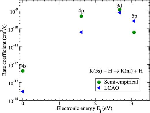
Rate coefficients for the (de-)excitation processes K(5s) + H → K(nl) + H at temperature T = 6000 K calculated by means of the model asymptotic semi-empirical approach (circles) and the asymptotic LCAO approach (triangles). The final states are shown at the corresponding electronic energies Ej of the potassium atom, see Table 1.
Since both the semi-empirical and the LCAO models perform roughly equally well on average, both sets of atomic data may be expected to have roughly the same accuracy. The two models pick up the same partial processes with the largest rate coefficients (within 10 per cent accuracy) and the processes with the moderate rates (typically within a factor of 1.3–5). The calculated atomic data provide reliable input for non-LTE modelling for stellar potassium spectra.
Very recently, a simplified model for estimating inelastic heavy-particle–hydrogen collision data has been proposed and applied to potassium-hydrogen collisions (Belyaev & Yakovleva 2017). This simplified model is derived for quick estimates of inelastic rate coefficients with minimal computational effort and presents a more approximate version of the semi-empirical approach used in this work. As a result, the simplified estimates are in good general agreement with the present results, but the present data have better accuracy.
4 RUBIDIUM-HYDROGEN COLLISIONS
4.1 Electronic structure
Rubidium is also an alkali and, hence, similar to potassium, although the atomic energy levels are slightly different, and this changes both the electronic structure and the inelastic rate coefficients. Again, the ground ionic molecular state has 1Σ+ symmetry, so the most important inelastic transitions occur within this symmetry. The five lowest (the ground and lowest lying excited) atomic rubidium states creating the 1Σ+ covalent molecular states, as well as the ionic molecular state, are collected in Table 3. Higher lying states are neglected since they produce negligibly small rate coefficients (for the same reasons as for K). In particular, one can see that the asymptotic ionic-state energy level for rubidium hydride is 0.159 eV lower than the corresponding level for potassium hydride and this shift is mainly responsible for differences in the electronic structure and the collision data.
RbH(1Σ+) scattering channels and asymptotic energies with respect to the ground state. The asymptotic energies of the scattering channels coincide with the corresponding electronic energy levels of the atom, which are adopted as J-averaged experimental values taken from NIST (Kramida et al. 2016).
| Scattering | Asymptotic | |
|---|---|---|
| j | channels | energies (eV) |
| 1 | Rb(5s 2S) + H(1s2S) | 0.0 |
| 2 | Rb(5p 2P) + H(1s2S) | 1.579 |
| 3 | Rb(4d 2D) + H(1s2S) | 2.400 |
| 4 | Rb(6s 2S) + H(1s2S) | 2.496 |
| 5 | Rb(6s 2P) + H(1s2S) | 2.947 |
| i | Rb+(1S) + H−(1s21S) | 3.427 |
| Scattering | Asymptotic | |
|---|---|---|
| j | channels | energies (eV) |
| 1 | Rb(5s 2S) + H(1s2S) | 0.0 |
| 2 | Rb(5p 2P) + H(1s2S) | 1.579 |
| 3 | Rb(4d 2D) + H(1s2S) | 2.400 |
| 4 | Rb(6s 2S) + H(1s2S) | 2.496 |
| 5 | Rb(6s 2P) + H(1s2S) | 2.947 |
| i | Rb+(1S) + H−(1s21S) | 3.427 |
Having the asymptotic limits of the ionic and low-lying covalent molecular states allow one to evaluate the low-lying long-range adiabatic potentials by means of the semi-empirical and the LCAO approaches. The most important for a non-adiabatic nuclear dynamics adiabatic potentials calculated in this work by means of both the semi-empirical and the LCAO approaches are plotted in Fig. 5. Since the rubidium energy structure is similar to that for potassium, the adiabatic potentials for these alkali hydrides are similar but not identical, see Figs 1 and 5. The series of the avoided crossings is clearly seen at long range. These non-adiabatic regions are most important for large and moderate inelastic rate coefficients in low-energy rubidium-hydrogen collisions. The profiles of the adiabatic potentials allow us to calculate the non-adiabatic Landau–Zener parameters in each non-adiabatic region by means of the adiabatic-potential-based formula (Belyaev & Lebedev 2011).
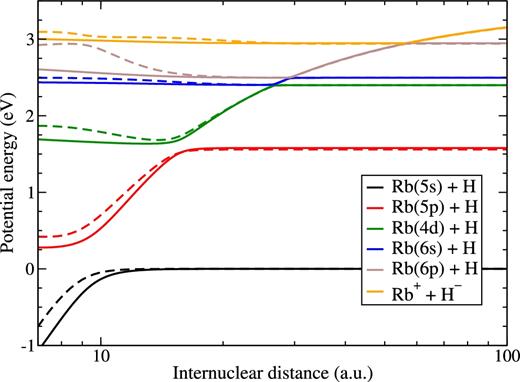
RbH(1Σ+) adiabatic potential energy curves obtained by means of the model semi-empirical approach (solid curves) and by the model LCAO approach (dashed curves).
The adiabatic potentials calculated in this paper by the model asymptotic approaches are in the general agreement with the accurate pseudo-potential results (Khelifi et al. 2002a) for rubidium hydride, but again the numerical data of Khelifi et al. (2002a) are not available and this prevents using the pseudo-potential data for a non-adiabatic nuclear dynamics in Rb + H collisions. The existing data for the ground molecular state of rubidium hydride, for example Geum et al. (2001), are again not sufficient for non-adiabatic dynamics. Other molecular symmetries of rubidium hydride are not included into the dynamical consideration, since they do not produce long-range non-adiabatic regions that could lead to substantial inelastic rate coefficients, see e.g. Khelifi et al. (2002a).
4.2 Non-adiabatic nuclear dynamics
The non-adiabatic nuclear dynamical treatment in rubidium-hydrogen collisions was performed in this work by means of the multichannel approach (Yakovleva et al. 2016). Finally, the state-to-state inelastic transition probabilities, partial inelastic cross-sections and rate coefficients were calculated. The rate coefficients for the temperature range T = 1000–10 000 K are presented as online supplementary material. Table 4 presents the inelastic rate coefficients for temperature T = 6000 K based on the two sets of the non-adiabatic parameters computed by means of the semi-empirical and the LCAO approaches. The value in the upper position of each cell of the table corresponds to the calculation with the semi-empirical parameters, while the value in the lower position to that with the LCAO parameters. Graphical representation of these data is plotted in Fig. 6.
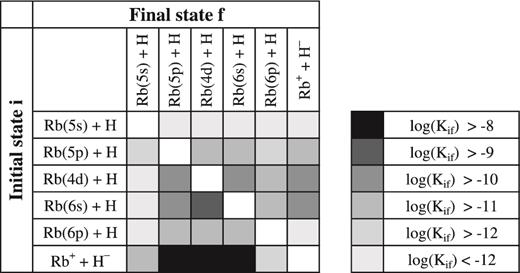
Graphical representation of the rate coefficients Kif (T) (in units of cm3 s−1) for the inelastic processes in Rb + H and Rb+ + H− collisions at temperature T = 6000 K calculated by means of the semi-empirical approach.
Rate coefficients, in units of cm3 s−1, at T = 6000 K for the excitation, de-excitation, ion-pair formation and mutual neutralization processes in rubidium-hydrogen collisions. In each cell of the table, the upper value corresponds to the rate coefficient calculated based on the adiabatic potentials obtained from the model semi-empirical approach, while the lower to the model LCAO approach.
| Initial | Final state | |||||
|---|---|---|---|---|---|---|
| state | Rb(5s) +H | Rb(5p) +H | Rb(4d) +H | Rb(6s) +H | Rb(6p) +H | Rb+ + H− |
| Rb(5s) +H | – | 2.34E-13 | 7.89E-15 | 3.62E-15 | 1.55E-16 | 1.80E-14 |
| – | 1.23E-13 | 9.61E-16 | 3.97E-16 | 2.37E-17 | 5.19E-15 | |
| Rb(5p) +H | 1.66E-12 | – | 5.55E-11 | 2.44E-11 | 1.65E-12 | 5.25E-11 |
| 8.42E-13 | – | 9.36E-12 | 3.64E-12 | 6.36E-13 | 2.18E-11 | |
| Rb(4d) +H | 1.64E-13 | 1.63E-10 | – | 2.45E-10 | 1.63E-11 | 2.72E-10 |
| 2.00E-14 | 2.86E-11 | – | 1.88E-10 | 5.62E-11 | 3.23E-10 | |
| Rb(6s) +H | 4.52E-13 | 4.31E-10 | 1.48E-09 | – | 6.20E-11 | 9.85E-10 |
| 4.98E-14 | 6.69E-11 | 1.13E-09 | – | 2.29E-10 | 1.16E-09 | |
| Rb(6p) +H | 1.54E-14 | 2.33E-11 | 7.84E-11 | 4.94E-11 | – | 3.01E-13 |
| 2.34E-15 | 9.21E-12 | 2.66E-10 | 1.80E-10 | – | 1.57E-12 | |
| Rb+ + H− | 5.45E-11 | 2.25E-08 | 3.97E-08 | 2.39E-08 | 9.15E-12 | – |
| 1.56E-11 | 9.64E-09 | 4.68E-08 | 2.78E-08 | 4.81E-11 | – | |
It is seen that again the mutual neutralization processes have the largest rate coefficients. The largest value of roughly 4 × 10⁻⁸ cm3 s−1 corresponds to the neutralization process into the Rb(4d) final state. The deviation between the results based on different electronic structure calculations is roughly 15 per cent. The largest value for the Rb+ + H− inelastic rate coefficient is roughly 30 per cent larger than the largest rate coefficient in K+ + H− collisions. The next largest rate coefficients correspond to the mutual neutralization processes into the Rb(6s) and Rb(5p) final states with the values exceeding 10−8 cm3 s−1. The mutual neutralization rate coefficients for different final states are shown in Fig. 7. It is seen from this figure (as well as from Table 4 and Fig. 6 ) that the rate coefficients for the neutralization process into the Rb(5s) and Rb(6p) final states are more than 2 orders of magnitude smaller. It is also seen that the different approaches provide values of the same order of magnitude.
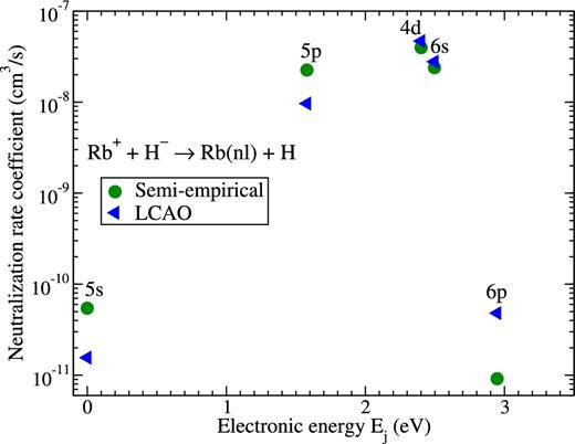
Rate coefficients for the mutual neutralization processes Rb+ + H− → Rb(nl) + H at temperature T = 6000 K calculated by means of the model asymptotic semi-empirical approach (circles) and the asymptotic LCAO approach (triangles). The final states are shown at the corresponding electronic energies Ej of the rubidium atom, see Table 3.
The inelastic rate coefficients for the excitation and de-excitation processes in Rb + H collisions are smaller than for the mutual neutralization processes. The largest rate is for the Rb(6s → 4d) transition. It is slightly exceeding 10−9 cm3 s−1 and roughly 30 times smaller than the maximum value for the neutralization process. The deviation between the results of using the different approaches is approximately 30 per cent for this rate. The example of the (de-)excitation rate coefficients in Rb(6s) + H collisions is shown in Fig. 8. The largest rates and the agreement between different approaches for these rates are clearly seen. One can also see that other (de-)excitation rate coefficients have much smaller values, especially for the transition from/to the ground state. The deviations between rates calculated by different approaches are larger for smaller rates, but remain within an order of magnitude estimate.
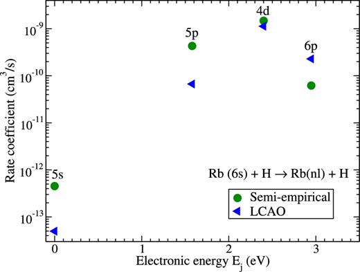
Rate coefficients for the (de-)excitation processes Rb(6s) + H → Rb(nl) + H at temperature T = 6000 K calculated by means of the model asymptotic semi-empirical approach (circles) and the asymptotic LCAO approach (triangles). The final states are shown at the corresponding electronic energies Ej of rubidium atom, see Table 3.
The two models single out the same partial processes with the largest rate coefficients (within 15 per cent accuracy) and the processes with the moderate rates (within a factor of 1.3–10). It is shown that both the semi-empirical and the LCAO approaches perform equally well on average and that both sets of atomic data have roughly the same accuracy. The calculated atomic data provide reliable input for non-LTE modelling for stellar rubidium spectra.
5 CONCLUSION
Cross-sectionsand rate coefficients for inelastic processes in low-energy K + H, K+ + H− and Rb + H, Rb+ + H− collisions for all transitions between 5 low-lying covalent states plus the ionic states (in each system) are calculated by means of the two quantum model approaches, the asymptotic semi-empirical and the asymptotic LCAO ones, for the electronic structures followed by the quantum multichannel approach for the non-adiabatic nuclear dynamics performed with two independent codes. Other (higher lying) covalent states have negligible rate coefficients.
In potassium-hydrogen collisions, the largest rate coefficients exceed 10−8 cm3 s−1 and are as large as 3.5 × 10⁻⁸ cm3 s−1 at T = 6000 K for the mutual neutralization processes into the K(5s 2S), K(3d 2D) and K(4p 2P) final states. For the two largest rate coefficients, the deviation between the results based on different electronic structure calculations are 10 per cent and 30 per cent, while for the third largest it is within a factor of 3. The rate coefficients for the (de-)excitation processes are typically much smaller than for the mutual neutralization, at least 30 times smaller than the maximum value for neutralization. The largest (de-)excitation rate corresponds to the K(5s → 3d) transition (excitation) reaching ≈10−9 cm3 s−1. The deviation between the rates calculated by the different model approaches for this partial process is ≈ 30 per cent. For other processes the rate coefficients are smaller, and the deviation gets larger, but agreement remaining within an order of magnitude; such partial processes with low rates are expected to be less important for non-LTE modelling.
In rubidium-hydrogen collisions, the largest rate coefficients exceed 10−8 cm3 s−1 and are as large as 4.7 × 10⁻⁸ cm3 s−1 at T = 6000 K for the mutual neutralization processes into the Rb(4d 2D), Rb(6s 2S) and Rb(5p 2P) states. This value (for Rb+ + H− collisions) is roughly 30 per cent larger than the largest rate coefficient in K+ + H− collisions. For the two largest rates, the deviation between the results of the different approaches is ≈ 15 per cent, for the third again within a factor of 3. The largest (de-)excitation rate coefficient in these collisions corresponds to the Rb(6s → 4d) de-excitation, has the value ≈1.5 × 10⁻⁹ cm3 s−1, which is roughly 50 per cent larger than the largest (de-)excitation rate in potassium-hydrogen collisions. The deviation for the Rb(6s → 4d) de-excitation rates calculated by the different approaches is again ≈ 30 per cent. For partial processes with smaller rates, the smaller the rates the larger the deviation, see e.g. Table 4, but order of magnitude agreement still remains.
The rate coefficients for the mutual neutralization, ion-pair formation, excitation and de-excitation processes are calculated for all transitions between the five lowest lying covalent states and the ionic states for each collisional system by means of the two quantum model approaches: semi-empirical and LCAO. The two model calculations single out the same partial processes with the largest rate coefficients (within ≈ 15 per cent accuracy) and the processes with moderate rates (within a factor of 1.3 – 10). The processes with the largest rate coefficients are the mutual neutralization into the K(5s 2S) and Rb(4d 2D) final states. It is shown that both the semi-empirical and the LCAO approaches perform equally well on average and that both the sets of atomic data have roughly the same accuracy. The processes with the large and moderate rate coefficients are likely to be important for non-LTE modelling. The processes involving the ground states K(4s 2S) and Rb(5s 2S), as well the high-lying K(5p 2P) and Rb(6s 2P) states have negligible rate coefficients. The processes with low rate coefficients are expected to be unimportant for astrophysical applications (Barklem 2016a). The present data provide a reliable basis for non-LTE stellar atmosphere modelling of the spectrum of rubidium and potassium.
Acknowledgements
AKB and SAY gratefully acknowledge partial support from the Ministry for Education and Science (Russian Federation), projects No. 3.5042.2017/6.7, 3.1738.2017/4.6. SAY also gratefully acknowledges partial support from the Dynasty Foundation (Russian Federation). PSB gratefully acknowledges the support of the Swedish Research Council. PSB is also supported by the project grant ‘The New Milky Way’ from the Knut and Alice Wallenberg foundation.
The data are available at the CDS via anonymous ftp to cdsarc.u-strasbg.fr (130.79.128.5) or via http://cdsweb.u-strasbg.fr/cgi-bin/qcat?J/MNRAS/XXX/XXX
REFERENCES
SUPPORTING INFORMATION
Supplementary data are available at MNRAS online.
Supplementary data are available at ReadMe.txt, KH_rt_semi_1000.dat, KH_rt_semi_2000.dat, KH_rt_semi_3000.dat, KH_rt_semi_4000.dat, KH_rt_semi_5000.dat, KH_rt_semi_6000.dat, KH_rt_semi_7000.dat, KH_rt_semi_8000.dat, KH_rt_semi_9000.dat, KH_rt_semi_10000.dat, KH_rt_LCAO_1000.dat, KH_rt_LCAO_2000.dat, KH_rt_LCAO_3000.dat, KH_rt_LCAO_4000.dat, KH_rt_LCAO_5000.dat, KH_rt_LCAO_6000.dat, KH_rt_LCAO_7000.dat, KH_rt_LCAO_8000.dat, KH_rt_LCAO_9000.dat, KH_rt_LCAO_10000.dat
Please note: Oxford University Press is not responsible for the content or functionality of any supporting materials supplied by the authors. Any queries (other than missing material) should be directed to the corresponding author for the article.
