


Abstract
We have developed a novel direct algorithm to derive the mass-ratio distribution (MRD) of short-period binaries from an observed sample of single-lined spectroscopic binaries (SB1s). The algorithm considers a class of parametrized MRDs and finds the set of parameters that best fits the observed sample. The algorithm consists of four parts. First, we define a new observable, the modified mass function, that can be calculated for each binary in the sample. We show that the distribution of the modified mass function follows the shape of the underlying MRD, making it more advantageous than the previously used mass function, reduced mass function or reduced mass function logarithm. Second, we derive the likelihood of the sample of modified mass functions to be observed given an assumed MRD. A Markov chain Monte Carlo search enables the algorithm to find the parameters that best fit the observations. Third, we propose that the unknown MRD is expressed by a linear combination of a basis of functions that spans the possible MRDs, and we suggest two such bases. Fourth, we show how to account for the undetected systems that have a radial-velocity amplitude below a certain threshold. Without the correction, this observational bias suppresses the derived MRD for low mass ratios. Numerous simulations show that the algorithm works well with either of the two suggested bases. The four parts of the algorithm are independent, but the combination of these four parts makes the algorithm highly effective at deriving the MRD of the binary population.
1 INTRODUCTION
The study of the mass-ratio distribution (MRD) of binaries, short-period binaries in particular, has a long history. This is because the MRD plays a key role in various aspects of the theory of binary formation and evolution. First, it provides one of the very few ways to challenge the theories of binary formation using observations (e.g. Bate & Bonnell 1997; Satsuka et al. 2017). Secondly, the primordial MRD is a one of the few major inputs for population syntheses of binaries (e.g. Toonen, Nelemans & Portegies Zwart 2012; Yungelson & Kuranov 2017), which try to predict, for example, the rate of supernova explosion and black hole mergers. Thirdly, the binary fraction and the MRD have been shown to play important roles in star cluster evolution (e.g. Hut et al. 1992; Benacquista & Downing 2013). Finally, an understanding of the low end of the MRD is crucial for the determination of the borders of the brown dwarf desert (e.g. Mazeh et al. 2003; Grether & Lineweaver 2006) that separates exoplanets from low-mass stellar secondaries.
It is therefore not surprising that quite a few studies have tried to derive the MRD of binaries, using short-period spectroscopic binaries (SBs) in particular. Reviews of the early studies can be found in Trimble (1990) and Mazeh & Goldberg (1992). Because some of these studies (e.g. Lucy & Ricco 1979; Duquennoy & Mayor 1991; Tokovinin 2000; Goldberg, Mazeh & Latham 2003; Fisher, Schröder & Smith 2005; Raghavan et al. 2010; Boffin 2010, 2015; Curé et al. 2015) yielded conflicting results, the shape of the MRD of short-period binaries continues to be an open question.
Derivations of the MRD should be based on a complete sample of binaries discovered by a systematic radial-velocity (RV) search. Generally, MRDs can depend on the mass of the primary star (Kouwenhoven et al. 2009), so analysed samples should be restricted to some narrow range of spectral types. In an ideal world, with spectra of unlimited resolution and signal-to-noise ratio, each SB would be a double-lined spectroscopic binary (SB2), with mass ratio derived directly from the ratio of the RV amplitudes of the two components. In reality, the derivation of the MRD of short-period binaries is based on samples for which most of the binaries observed are single-lined spectroscopic binaries (SB1s), where only the RVs of the primary star can be measured. Even after obtaining observations of a large sample of SB1s, the derivation of the MRD is hampered by the fact that for each of the SB1s, the orbital solution cannot yield the mass ratio itself but merely the mass function, which is a combination of two unknowns: the mass ratio and the plane-of-motion inclination angle. Therefore, a statistical approach must be applied to the observational results, assuming random distribution of the orbital inclination of the sample as a whole.
Two main approaches have been used to disentangle the MRD from the orbital inclination (e.g. Heacox 1995). In the inverse approach, we consider the sample of derived mass functions and work back, usually iteratively (see the classical work of Lucy 1974), to the underlying MRD of the binary population (e.g. Lucy & Ricco 1979; Mazeh & Goldberg 1992; Boffin 2010; Curé et al. 2015).
In the direct approach, however, we assume a certain MRD of the binary population, calculate the resulting expected distribution of some observable O, and compare it with the set of {Oi} obtained from the sample of SB1s, where the ith binary is represented by Oi. Then, we find the MRD that best fits the observed set {Oi} (e.g. Hogeveen 1992; Tokovinin 1992; Ducati, Penteado & Turcati 2011). The comparison between the expected distribution and the observed sample is usually done by comparing histograms, not a very powerful approach, which does not allow statistical derivation of the best parameter(s) of the MRD and its (their) confidence intervals.
In previous studies, the observable used was the reduced mass function y, obtained by dividing the mass function by the mass of the primary star; however, see Lucy & Ricco (1979) and Boffin (2010, 2015), who promoted the use of a logarithm of the observable instead. However, we will show that the expected distributions of both y and log y for very different MRDs are similar, making the derivation of the true MRD difficult.
Here we present a novel algorithm to solve the problem, which consists of four parts. First, we introduce a new observable S, which we call the ‘modified mass function’, that is derived for each SB1. We then show that the shape of the distribution of the obtained S for a binary sample is similar to that of the underlying MRD of the population. Even more importantly, different MRDs result in different S-distributions.
Secondly, we suggest a comparison of the expected distribution of S with the observed sample by deriving the likelihood of the observed set of {Si}, given the assumed MRD (see also Tokovinin 1992). We can then find the parameters of the MRD that maximize the likelihood of observing the sample, using a Markov chain Monte Carlo (MCMC) approach, for example.
Thirdly, we suggest that the unknown MRD is expressed by a linear combination of a basis of functions, with some unknown coefficients. We then search for the coefficients that maximize the likelihood of the observed sample.
Fourthly, following Mazeh & Goldberg (1992) we show how to account for the undetected binaries that have an RV amplitude below a certain threshold. Without the correction, this observational bias suppresses the derived MRD for low mass ratios.
In Section 2, we introduce the modified mass function. In Section 3, we detail the search for the best set of parameters using the MCMC process, and we suggest two sets of functions. In Section 4, we detail two simulated examples, which demonstrate that the algorithm works well. In Section 5, we present our correction function. In Section 6, we briefly summarize this work and lay out possible further refinements of the algorithm. In the following series of papers, we will apply the algorithm to various SB1 samples.
2 THE MODIFIED MASS FUNCTION
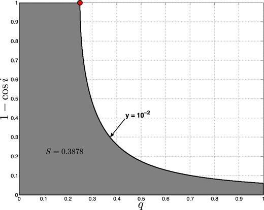
The (1 − cos i, q) parameter space, with an SB1 with y = 10−2. The grey area shows the corresponding S value. The red dot marks the minimum value of q (i.e. |$\mathcal {Q}_{y}$|), which is 0.25.
Previous techniques used the observables y or log y as tools for deriving the MRD. For the direct method, it is necessary to obtain the probability density function (PDF) of y, fy or flog y, given the PDF of the MRD, fq. To obtain fy(y; fq), we have to calculate the probability of obtaining a value between y and y + dy over the parameter space of Fig. 1, given fq(q). This is done in Appendix A.
We seek a transformation |$S=\mathbb {S}(y)$| such that significant functional properties of the MRD, fq, will be qualitatively demonstrated by its resulting PDF, fS. This results in three requirements. First, a uniform fq should yield a uniform fS. Secondly, the transformation |$\mathbb {S}$| is required to be strictly increasing and continuous. Finally, for fS to be comparable with fq, the range of |$\mathbb {S}$| is required to be the [0, 1] interval.
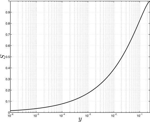
Modified mass function S as a function of the reduced mass function y.
The modified mass function, by its definition, resembles a copula (e.g. Nelsen 2013). While copulas are widely used in many fields, especially in quantitative finance, its astrophysical applications are rare (e.g. Scherrer et al. 2010). A detailed derivation of |$\mathbb {S}$| appears in Appendix B.
2.1 Distribution of the modified mass function
Fig. 3 shows the derived fy and fS for three different simple fq functions, demonstrating how, unlike fy or flog y, fS captures the shape of the underlying MRD, fq.
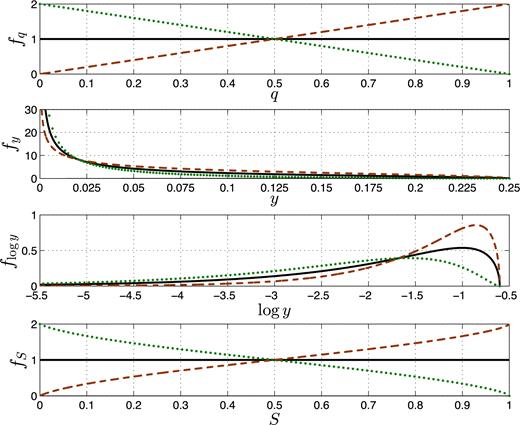
Three distributions of q and their corresponding y, log y and S distributions. The top panel shows the uniform (black line), linearly increasing (brown dashed line) and decreasing (green dotted line) distributions of q. The three lower panels show the corresponding y, log y and S distributions, with the same line types and colours.
3 DIRECT DERIVATION OF THE MRD
3.1 Likelihood derivation of the MRD
Let us assume that the MRD is characterized by a set of parameters |${\boldsymbol {c}}=\lbrace c_k\rbrace$|. This could be, for example, a Gaussian distribution |$f_q\propto \exp [ (q-c_1)^2/2c_2^2 ]$|, a power-law distribution |$f_q\propto q^{c_1}$|, a flat distribution between c1 = qmin and c2 = qmax, and such like, or any combination of the above. Using equation (8), we transform the |$f_q(q;{\boldsymbol {c}})$| into |$f_S(S;{\boldsymbol {c}})$|, which has the same set of parameters {ck}.
3.2 Expansion of MRD by a set of basis functions
In the following subsections, we suggest two possible sets of basis functions: the shifted Legendre polynomials and the boxcar functions. The two have complementary properties in terms of smoothness and locality. Obviously, other possibilities, such as harmonic functions or power series, can be considered and implemented in a similar manner.
3.2.1 Shifted Legendre polynomials
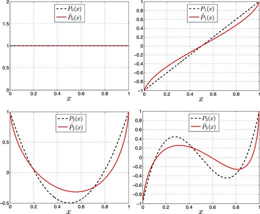
First four shifted Legendre polynomials (dashed black) and their corresponding modified functions (solid red).
The shifted Legendre polynomials have the property |$\int _0^1 P_k(x)\, {\rm d}x = \delta _{k0}$|. This makes them suitable as a set of basis function for any PDF, as the integral of any combination of them over the range [0, 1] is unity, as long as c0 = 1.
3.2.2 Boxcar functions
3.3 Starting point of the MCMC
In any MCMC search, it is important to start the chain not too far from the global maximum of the log-likelihood. Our starting point relies on the histogram of observed {Si}. For the boxcar basis, the starting point is taken as the normalized number of counts in the S histogram bins, whereas the starting point of the Legendre polynomial set was derived by a simple linear least-squares fit to the histogram bins (see Barlow 1989).
4 TESTING THE ALGORITHM
In order to test our algorithm, and the two bases presented above in particular, we ran numerous simulations, two of which are presented here. In each numerical experiment, we assumed an underlying MRD and prepared a simulated SB1 sample, drawing at random the values for the mass ratio and the inclination of each binary. We then derived the S value for each binary and applied our algorithm to the sample of modified mass functions twice, using at each time one of our two bases.
In all our simulations, we were able to retrieve the correct shape of the underlying MRD, with each of the two bases.
Here we present two simulations, one (Fig. 5) with an MRD composed of a fourth-degree polynomial, fq(q) ∝ 25(2q − 1)4 + 4, that peaks at q = 0 and q = 1, and the other (Fig. 6) composed of a Gaussian with a mean at q = 0.2 and a standard deviation of 0.15 (77 per cent of the population) together with a flat distribution in the range q = [0, 1] (23 per cent). Because, typically, the number of SBs in modern spectroscopic surveys is of the order of 100 – for example, Goldberg et al. (2003) analysed 129 SBs – we chose the size of the simulated sample to be 100 SB1 systems in both examples.
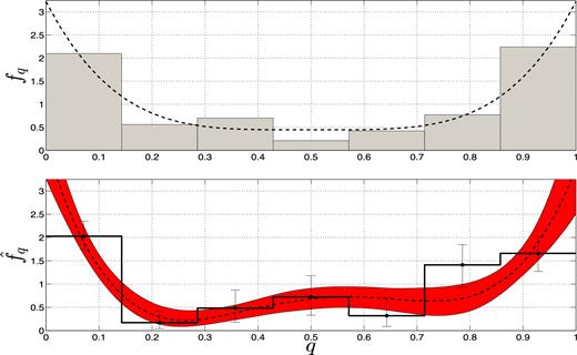
Derivation of MRDs from a simulation of a sample of 100 SB1s. The top panel shows the simulated sample of 100 SB1s, with random orientations, using as an MRD (dashed black line) a fourth-degree polynomial, fq(q) ∝ 25(2q − 1)4 + 4, that peaks at q = 0 and q = 1. The specific drawn sample is presented by a seven-bin histogram. The bottom panel shows two independently derived MRDs, one using the first five shifted Legendre polynomials as a basis (dashed black line) and the other using the boxcar basis of seven bins (thick black line). Each derived MRD is associated with an error for each value of q (see text).
![Derivation of MRDs from a simulation of a sample of 100 SB1s. The simulated MRD is composed of a Gaussian with a mean at q = 0.2 and width of 0.15 (77 per cent of the population) and a flat part in the range q = [0, 1] (23 per cent). The simulated sample and the two derived MRDs are plotted as in Fig. 5.](https://oup.silverchair-cdn.com/oup/backfile/Content_public/Journal/mnras/472/4/10.1093_mnras_stx2257/2/m_stx2257fig6.jpeg?Expires=1749927259&Signature=JBRSdi1sQo1quOTqBpGhAf7rdr7hFP-dry3K~xbJnqh6~VPcowl4SDrO4Ia8oDRqPQ3pNDXLBIiL-zww9q2NxdF-8JkPcM4Sp5C1FJ70~yRfYcVUMq9U2wFvknNmOuIoLyo5vVpdxQKyOc88uW3uZQNYUq0Q-3rHno5LTCkT~W9HDGIaCeVK8wLmETM~ty~1vu3qB7qtvVEm3li7OKVL1cnO7ZVObV99H4uhqYslbAOEBT7V-Ub942qczB84jt4YBgnXgd1Pf2zmiHk72DUFIopzHXdW5yZWsQOG4RJcYSY1KCb2pVi8iV69w6vtu-UoVwh0voL2c4qTuc-mNE2uSw__&Key-Pair-Id=APKAIE5G5CRDK6RD3PGA)
Derivation of MRDs from a simulation of a sample of 100 SB1s. The simulated MRD is composed of a Gaussian with a mean at q = 0.2 and width of 0.15 (77 per cent of the population) and a flat part in the range q = [0, 1] (23 per cent). The simulated sample and the two derived MRDs are plotted as in Fig. 5.
The best MRD model and its uncertainty were derived by calculating the median and scatter of the values obtained for each q along the MCMC run, as described in Section 3.1. The top panels of Figs 5 and 6 show the MRD used and the mass-ratio histogram of the simulated sample, while the bottom panels present the MRDs derived with a basis of seven boxcar functions and with the first five shifted Legendre polynomials.
The two examples demonstrate the power of our algorithm, as the derived MRDs are very close to the underlying functions, even though the algorithm was applied without any assumption on the shape of the MRD.
5 ACCOUNTING FOR AN OBSERVATIONAL DETECTION THRESHOLD
Samples of observed spectroscopic binaries are subjected to many observational biases. An obvious bias (e.g. Mazeh & Goldberg 1992; Tokovinin 1992) is the detection threshold – RV surveys can identify SB systems only if their RV amplitude is large enough. The impact of such a selection effect becomes increasingly significant for small values of q, causing the derived |$\hat{f_q}$| at small q values to be underestimated. In this section, we describe our way to account for this observational bias, following the approach of Mazeh & Goldberg (1992).
Again, to test the correcting part of the algorithm, we ran numerous simulations, one of which is presented in Fig. 7. Here, we used the same population as in Fig. 5, but now with a 1-M⊙ primary for each binary, orbital periods with log-uniform distribution between 1 and 103 d, and a detection threshold of Kmin = 3 km s−1, which caused 22 simulated binaries not to be detected. A histogram of the detected and missed binaries is plotted in the top panel of Fig. 7. As can be seen in the figure, most of the missed binaries had low mass ratio, as expected. The lower panel shows the uncorrected and corrected distributions. The uncorrected MRD suffers from serious suppression of its lower part, while the correction succeeded in producing the correct underlying MRD. As expected, for small mass ratios, q ≲ 0.05, the correction factor |$1/\overline{D}(q)$| became large, and therefore we refrained from obtaining the corrected function for this range of q.
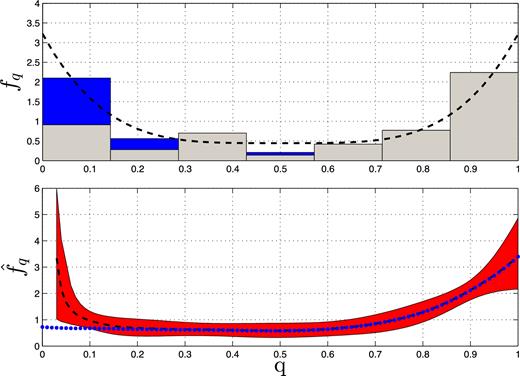
MRD derivation from a simulated SB1 sample with a detection threshold of Kmin = 3 km s−1. The top panel shows a simulated sample of 100 SB1s with random orientations, using an MRD (dashed black line) that peaks at q = 0 and q = 1. The specific drawn sample is presented by a seven (grey) bin histogram (see Fig. 5). Because of the detection threshold, the upper bins of 22 systems (blue) were not detected. The bottom panel shows the derived MRDs (dotted line), using the first five shifted Legendre polynomials as a basis, together with the corrected MRD (dashed line) and its confidence 1σ range (see text).
Another way to correct for the undetected binaries, not presented here, is to apply the derived |$\overline{D}(q)$| factor to the base functions, and to use these corrected functions along the MCMC fitting. One then constructs the true MRD by using the uncorrected base functions with the parameters obtained with the MCMC.
6 CONCLUSIONS
We have presented a novel direct algorithm to derive the MRD of short-period binaries from an observed SB1 sample. The algorithm considers a parametrized family of MRDs and finds the set of parameters that best fits the observed sample.
The algorithm consists of four parts. First, we define a new observable, the modified mass function S, derived for each SB1 in the sample. We show that the distribution of the modified mass function of an SB1 sample follows the shape of the underlying MRD, making the use of the modified mass function more advantageous than the previously used mass function, reduced mass function or the reduced mass function logarithm. Secondly, given an assumed MRD, we derive the likelihood of obtaining the observed sample of SB1s with the derived modified mass functions. Maximizing this likelihood by an MCMC search enables the algorithm to find the best parameters of the underlying MRD. Thirdly, we suggest that the unknown MRD is expressed by a basis of functions with some unknown coefficients that linearly span the space of possible MRDs. We suggest two such bases. Fourthly, we have shown how to account for the undetected systems that have an RV amplitude below a certain threshold. The correction is calculated per mass ratio and therefore can be applied to the derived MRD. Without the correction, this observational bias suppresses the derived MRD for low mass ratios. Numerous simulations show that the algorithm works with either of the two bases.
The algorithm is based on three simplifications. We consider only circular orbits, we ignore the double-lined binaries and we assume that there are no uncertainties associated with y and therefore with S. With the present layout, it is straightforward to generalize the algorithm to include eccentric orbits and uncertainties in S. However, it is an obvious drawback to ignore the extra information about the known mass ratio of the SB2s (e.g. Mazeh et al. 2003; Prato 2007; Fernandez et al. 2017). A further development of the algorithm to use the SB2 information is planned for a further publication. At present, the algorithm treats those systems as SB1s.
The detection threshold correction presented here depends on the orbital period distribution of the binary population and on the assumption that the MRD does not depend on the binary period; see the discussion by Moe & Di Stefano (2017), which put this assumption into question for O- and B-type stars. These two assumptions are inherent to any correction algorithm, as the RV amplitude does depend on the mass ratio and the orbital period. The simulations show that the correction succeeded in producing the correct MRD for low mass ratios.
The correction is based on a simplistic conception of the detection threshold. In reality, the observational bias does not act as a stiff threshold, but instead the detection probability of a binary is a continuous monotonic increasing function of its amplitude, which depends on the period, determined by the time stamp of the RV observations. However, it is easy to adopt the algorithm for any detection sensitivity through equations (22) and (23), by which one can derive a more sophisticated correction for any value of mass ratio. Needless to say, any derivation of the MRD can be based only on a sample that was obtained by a complete systematic survey that searches for spectroscopic binaries with known detection thresholds, so that the corrections can be derived and applied to the observed sample.
Obviously, the correction procedure introduces additional errors to the derived MRD, because of the inexact period distribution and inaccurate detection threshold used. Therefore, the correction becomes less valuable for low mass ratios, a range for which we have a small number of systems and for which the correction factor becomes large. In the simulated case presented above, for example, we refrained from plotting the corrected MRD for mass ratio smaller than 0.05. The exact limit depends on the specific SB1 sample.
In the next paper of this series (Shahaf et al., in preparation), we apply the algorithm to a few samples published in the literature, in particular those of Mazeh et al. (2003), Fisher et al. (2005), Prato (2007), Mermilliod et al. (2007) – see also North (2014) and Van der Swaelmen et al. (2017) – and Tal-Or, Faigler & Mazeh (2015).
Furthermore, in the near future we anticipate extremely large new samples of SBs coming from the APO Galactic Evolution Experiment (APOGEE)1 and the Gaia2 project. The release of the Gaia distances will enable us to better estimate the primary masses of these samples, which is a key element in the derivation of the reduced and modified mass functions. The new algorithm will be ready for these large samples to determine the MRDs of SBs. In addition, we anticipate two additional large samples, which will explore binaries with very short and very long period ranges: eclipsing binaries from large photometric data bases – see, for example Mazeh, Tamuz & North (2006) and Mowlavi et al. (2017) for the analysis of the OGLE LMC binaries – and astrometric binaries from Gaia. The new samples will finally give us the full picture of the different binary populations.
Acknowledgements
We are indebted to the referee for the thorough reading of the manuscript and very helpful comments. We thank Shay Zucker for the insightful discussions. We acknowledge support from the Israel Science Foundation (grant No. 1423/11) and the Israeli Centers of Research Excellence (I-CORE, grant No. 1829/12).
REFERENCES
APPENDIX A: DISTRIBUTION OF THE REDUCED MASS FUNCTION
A rigorous development of the y PDF, fy, for a sample of randomly oriented binaries has been previously presented by Heacox (1995). Nevertheless, an alternative geometrical derivation of this might be instructive in the context of this work.
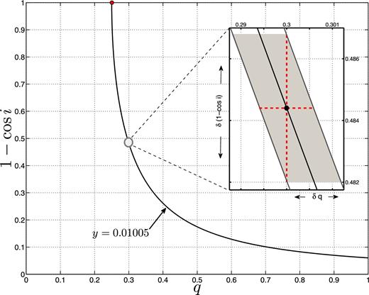
A contour of y = 0.01005 plotted in the (1 − cos i), q) plane. The red dot corresponds to the q minimum value of y = 0.01005. The grey circle indicates the point where q = 0.3. The enlarged window shows the area bounded by 0.0100 ≤ y ≤ 0.0101. The horizontal width of the parallelogram, δq, equals 0.0012 (dashed red). The vertical height of the parallelogram, δ(1 − cos i), equals |$\mathbb {K}(y,q)\times \delta y = 0.0047$| (dashed red).
APPENDIX B: DERIVATION OF THE MODIFIED MASS FUNCTION
The modified mass function S is required to be a strictly increasing continuous transformation of y, from [0, 0.25] on to [0, 1]. Additionally, if the underlying MRD fq is uniform, then its resulting S distribution fS is also required to be uniform.
|$\mathbb {S}$| is unique. Let |$\mathbb {T}$| and |$\mathbb {S}$| uphold the stated requirements. Because both are transformations of y, the PDFs obey fS|dS/dy| = fT|dT/dy|. Specifically for uniform fq, this relation becomes |dS/dy| = |dT/dy|. Because both are strictly increasing and continuous from [0, 0.25] on to [0, 1], |$\mathbb {T} \equiv \mathbb {S}$|.
