


Abstract
We report the joint WASP/KELT discovery of WASP-167b/KELT-13b, a transiting hot Jupiter with a 2.02-d orbit around a V = 10.5, F1V star with [Fe/H] = 0.1 ± 0.1. The 1.5 RJup planet was confirmed by Doppler tomography of the stellar line profiles during transit. We place a limit of <8 MJup on its mass. The planet is in a retrograde orbit with a sky-projected spin–orbit angle of λ = −165° ± 5°. This is in agreement with the known tendency for orbits around hotter stars to be more likely to be misaligned. WASP-167/KELT-13 is one of the few systems where the stellar rotation period is less than the planetary orbital period. We find evidence of non-radial stellar pulsations in the host star, making it a δ-Scuti or γ-Dor variable. The similarity to WASP-33, a previously known hot-Jupiter host with pulsations, adds to the suggestion that close-in planets might be able to excite stellar pulsations.
1 INTRODUCTION
There are far fewer hot-Jupiter exoplanets known to transit hot stars with Teff > 6700 K than those transiting later-type stars. This is partially a selection effect given that planets transiting very hot or fast-rotating stars are harder to validate, since the lack of spectral lines makes it harder to obtain accurate radial-velocity measurements. Thus, radial-velocity surveys have tended to avoid hotter stars, while transit searches such as the Wide Angle Search for Planets (WASP) have, in the past, paid less attention to such candidates.
Hot Jupiters are often in orbits that are not aligned with the stellar rotation axis. One explanation is that hot Jupiters migrate within a disc which is itself tilted with respect to the stellar rotation axis, possibly due to a companion (Crida & Batygin 2014; Fielding et al. 2015). Another is that hot Jupiters arrive at their current orbits through high-eccentricity migration, owing to perturbations by third bodies (e.g. Dong, Katz & Socrates 2014), which leads to a range of orbital obliquities.
The planets that have been found around hotter stars have a greater tendency to be in misaligned orbits, compared to planets orbiting later-type stars (Winn et al. 2010; Albrecht et al. 2012), suggesting a systematic difference in their dynamical history. In addition there appears to be a dearth of hot Jupiters orbiting very fast rotators, such that the star rotates faster than the planetary orbit (e.g. Wu & Murray 2003; Fabrycky & Tremaine 2007; McQuillan, Mazeh & Aigrain 2013), though this may again be partially a selection effect. In such stars the usual tidal decay of a hot Jupiter orbit would be reversed, provided the orbit is prograde, again changing the dynamical history.
For such reasons the WASP (Pollacco et al. 2006; Hellier et al. 2011) and KELT (Kilodegree Extremely Little Telescope: Pepper et al. 2007, 2012) transit-search teams are now giving more attention to hotter candidates. The first hot Jupiter found to transit an A-type star was WASP-33b, where the planet was validated, not by radial-velocity measurements, but by the detection of the shadow of the planet seen through tomography of the stellar line profiles during transit (Collier Cameron et al. 2010b). This technique requires a higher signal-to-noise ratio than radial-velocity measurements, and thus a bigger telescope for a given host-star magnitude.
Tomographic methods have since led to the detection of the hot Jupiters KELT-17b (Zhou et al. 2016), HAT-P-57b (Hartman et al. 2015), XO-6b (Crouzet et al. 2017), HAT-P-67b (Zhou et al. 2017) and most recently KELT-9b (Gaudi et al. 2017), as well as the warm Jupiter Kepler-448b (Bourrier et al. 2015). The hot Jupiter Kepler-13 Ab has also been detected tomographically (Johnson et al. 2014), though in that case the planet's existence had previously been confirmed using the orbital phase curve (Shporer et al. 2011; Mazeh et al. 2012).
In this work, we present the joint WASP/KELT discovery of a transiting hot Jupiter dubbed WASP-167b/KELT-13b. The planet host star is a 7000 K, rapidly rotating (v sin i⋆ ≈50 km s−1) F1V star.
2 DATA AND OBSERVATIONS
WASP-167b/KELT-13b was observed with WASP-South from 2006 May to 2012 June and with KELT-South from 2010 March to 2013 August. WASP-South is an eight-camera array using 200-mm f/1.8 lenses, covering a 7.8° × 7.8° field of view. Typically eight fields per night were observed with a broad-band filter (400–700 nm) using 30-s exposures and typically 10-min cadence. Details of the data reduction and processing are given by Collier Cameron et al. (2006) and an explanation of the process for selecting candidates is given by Collier Cameron et al. (2007).
The KELT-South site consists of a single 80-mm f/1.9 camera with a 26° × 26° field of view and a pixel scale of 23 arcsec. Survey observations use 150-s exposures and a cadence of 10–20 min per field. Further details of KELT-South are given in Pepper et al. (2012). Details of the data reduction, processing and candidate selection procedures are given by Siverd et al. (2012) and Kuhn et al. (2016).
The WASP and KELT teams independently found a planet-like transit signal with a ∼2-d period (see Fig. 1) and set about obtaining a total of 18 follow-up light curves of the transit. The observations are listed in Table 1 while the light curves are shown in Fig. 2. The techniques for obtaining relative photometry have been reported in previous WASP and KELT discovery papers, and since we have 18 transit curves from disparate facilities we refer the reader to such papers for full details of the instrumentation and analysis (e.g. Hellier et al. 2014; Kuhn et al. 2016; Maxted et al. 2016; Rodriguez et al. 2016; Pepper et al. 2017). We give key details of the instrumentation used in Table 1.
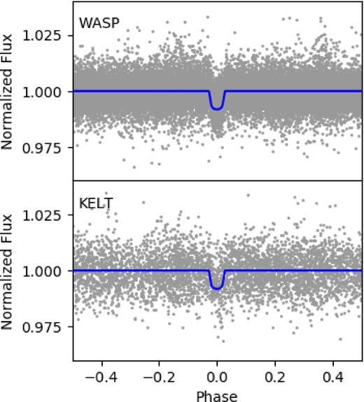
The WASP (top) and KELT (bottom) discovery light curves for WASP 167b/KELT-13b, folded on the orbital period. The blue lines show the final model obtained in the MCMC fitting (see Section 4).

Details of all observations of WASP-167b/KELT-13b used in this work, including the discovery photometry, the follow-up photometry and the spectroscopic observations. The label in the final column corresponds to a light curve in Fig. 2.
| Facility | Location | Aperture | FOV | Pixel scale | Date | Notes | Label |
|---|---|---|---|---|---|---|---|
| (΄ × ΄) | (arcsec pixel−1) | ||||||
| Discovery photometry | |||||||
| WASP-South | SAAOa, South Africa | 111 mm | 7.8 × 7.8 | 14 | 2006 May– | 26114 points | – |
| 2012 June | |||||||
| KELT-South | SAAO, South Africa | 42 mm | 26 × 26 | 23 | 2010 March– | 4563 points | – |
| 2013 August | |||||||
| Transit observations | |||||||
| TRAPPIST | ESOb, La Silla, Chile | 0.6 m | 22 × 22 | 0.65 | 2012 February 22 | I+z’ | a |
| TRAPPIST | ESO, La Silla, Chile | 0.6 m | 22 × 22 | 0.65 | 2012 April 30 | I+z’ | b |
| LCOGT-LSC | CTIOc, Chile | 1 m | 26.5 × 26.5 | 0.4 | 2014 May 17 | i’ | c |
| PEST | Perth, Australia | 0.3 m | 31 × 21 | 1.2 | 2014 June 22 | Rc | d |
| PEST | Perth, Australia | 0.3 m | 31 × 21 | 1.2 | 2015 January 14 | V | e |
| Skynet/Prompt4 | CTIO, Chile | 0.4 m | 10 × 10 | 0.59 | 2015 February 22 | z’ | f |
| T50 Telescope | SSOd, Australia | 0.43 m | 16.2 × 15.7 | 0.92 | 2015 March 24 | B | g |
| T50 Telescope | SSO, Australia | 0.43 m | 16.2 × 15.7 | 0.92 | 2015 March 26 | B | h |
| Mt. John | UCe, New Zealand | 0.6 m | 14 × 14 | 0.549 | 2015 March 26 | V | i |
| LCOGT-COJ | SSO, Australia | 1 m | 15.8 × 15.8 | 0.24 | 2015 March 28 | r’ | j |
| PEST | Perth, Australia | 0.3 m | 31 × 21 | 1.2 | 2015 March 28 | Ic | k |
| LCOGT-COJ | SSO, Australia | 1 m | 15.8 × 15.8 | 0.24 | 2015 March 28 | i’ | l |
| Hazelwood | Victoria, Australia | 0.32 m | 18 × 12 | 0.73 | 2015 March 30 | B | m |
| Ivan Curtis | Adelaide, Australia | 0.235 m | 16.6 × 12.3 | 0.62 | 2015 March 30 | V | n |
| Ellinbank | Victoria, Australia | 0.32 m | 30.4 × 14.1 | 1.12 | 2015 April 03 | B | o |
| PEST | Perth, Australia | 0.3 m | 31 × 21 | 1.2 | 2015 April 03 | B | p |
| LCOGT-CPT | SAAO, South Africa | 1 m | 15.8 × 15.8 | 0.24 | 2015 April 17 | Z | q |
| TRAPPIST | ESO, La Silla, Chile | 0.6 m | 22 × 22 | 0.65 | 2016 March 01 | z’ | r |
| Occultation window observations | |||||||
| TRAPPIST | ESO, La Silla, Chile | 0.6 m | 22 × 22 | 0.65 | 2011 February 13 | z’ | - |
| TRAPPIST | ESO, La Silla, Chile | 0.6 m | 22 × 22 | 0.65 | 2011 April 25 | z’ | - |
| TRAPPIST | ESO, La Silla, Chile | 0.6 m | 22 × 22 | 0.65 | 2011 May 09 | z’ | - |
| Spectroscopic Observations | |||||||
| CORALIE | ESO, La Silla, Chile | 1.2 m | – | – | 2010 April– | 21 RVs | - |
| 2017 March | |||||||
| TRES | FLWOf, Arizona | 1.5 m | – | – | 2015 February– | 20 RVs | - |
| 2016 April | |||||||
| HARPS | ESO, La Silla, Chile | 3.6 m | – | – | 2016 March 01 | 17 CCFs | - |
aSouth African Astronomical Observatory, bEuropean Southern Observatory, cCerro Tololo Inter-American Observatory, dSiding Spring Observatory, eUniversity of Canturbury, fFred Lawrence Whipple Observatory.
In an attempt to refute the planetary hypothesis we, on three occasions, attempted to detect an eclipse (of the occulting body by the star) using TRAPPIST with a z΄ filter (see Table 1 for details). This is discussed in Section 4.
The two teams also began monitoring the radial velocity of the star using the Euler/CORALIE and TRES spectrographs (Queloz et al. 2001; Fűresz 2008). The measured values are listed in Table 2. The crucial tomographic data, revealing the planet shadow, then came from an observation over a transit on the night of 2016 March 1 using the ESO 3.6-m/HARPS spectrograph (Pepe et al. 2002).
Radial velocities and bisector spans for WASP-167b/KELT-13b.
| BJD | RV | σRV | BS | σBS |
|---|---|---|---|---|
| (TDB) | (km s−1) | (km s−1) | (km s−1) | (km s−1) |
| TRES RVs: | ||||
| 2457055.9950 | −1.01 | 0.41 | −0.12 | 0.33 |
| 2457057.0280 | 0.00★ | 0.23 | 0.03 | 0.21 |
| 2457058.0115 | −0.57 | 0.28 | 0.53 | 0.37 |
| 2457060.9845 | −0.39 | 0.31 | 0.33 | 0.21 |
| 2457086.9123 | −0.63 | 0.29 | 0.04 | 0.24 |
| 2457122.8138 | −1.85 | 0.42 | −0.05 | 0.17 |
| 2457123.8544 | −1.15 | 0.39 | −0.23 | 0.28 |
| 2457137.7848 | −2.39 | 0.24 | −0.29 | 0.14 |
| 2457139.7803 | −2.00 | 0.39 | 0.15 | 0.24 |
| 2457141.7805 | −1.27 | 0.45 | 0.17 | 0.11 |
| 2457143.7671 | −2.19 | 0.23 | 0.17 | 0.14 |
| 2457144.7561 | −1.81 | 0.35 | −0.05 | 0.18 |
| 2457145.7548 | −1.39 | 0.32 | −0.02 | 0.16 |
| 2457149.7475 | −1.16 | 0.42 | 0.12 | 0.25 |
| 2457150.7423 | −2.33 | 0.44 | 0.05 | 0.20 |
| 2457151.7486 | −1.19 | 0.44 | −0.20 | 0.23 |
| 2457152.7481 | −2.52 | 0.36 | −0.29 | 0.18 |
| 2457406.0418 | −1.03 | 0.34 | − | − |
| 2457491.8087 | −0.84 | 0.34 | − | − |
| 2457504.7985 | −1.62 | 0.28 | – | – |
| CORALIE RVs: | ||||
| 2455310.5205 | −3.82 | 0.059 | −2.38 | 0.12 |
| 2455310.8005 | −3.74 | 0.061 | −0.42 | 0.12 |
| 2455311.8282 | −2.83 | 0.059 | −1.30 | 0.12 |
| 2455320.5338 | −3.50 | 0.063 | 1.80 | 0.13 |
| 2455320.7628 | −2.23 | 0.066 | −2.30 | 0.13 |
| 2455568.8079 | −2.72 | 0.060 | −2.70 | 0.12 |
| 2455572.8753 | −3.09 | 0.066 | − | − |
| 2455574.8568 | −3.57 | 0.061 | −4.96 | 0.12 |
| 2455646.7729 | −2.51 | 0.070 | −2.96 | 0.14 |
| 2455712.5532 | −3.36 | 0.059 | 0.26 | 0.12 |
| 2455722.5360 | −2.27 | 0.058 | −4.94 | 0.12 |
| 2455979.6816 | −3.76 | 0.062 | −3.44 | 0.12 |
| 2455979.8955 | −3.74 | 0.059 | −7.50 | 0.12 |
| 2455981.7270 | −4.62 | 0.065 | −1.09 | 0.13 |
| 2457600.5011 | −4.28 | 0.071 | − | − |
| 2457616.4971 | −4.70 | 0.066 | 0.048 | 0.13 |
| 2457759.8370 | −4.71 | 0.065 | −1.86 | 0.13 |
| 2457760.8366 | −3.77 | 0.066 | −3.70 | 0.13 |
| 2457804.7057 | −4.08 | 0.065 | − | − |
| 2457809.7750 | −5.18 | 0.064 | −2.88 | 0.13 |
| 2457818.6607 | −4.73 | 0.067 | −0.25 | 0.13 |
★This observation was used as the template for the extraction of the TRES radial velocities.
We have searched the combined WASP and KELT photometry of WASP-167/KELT-13 for modulations indicating the rotational period of the star, as described by Maxted et al. (2011), but did not find any modulations above ∼0.7 mmag at periods longer than 1 d.
3 SPECTRAL ANALYSIS
To determine the spectral parameters of the host star, we produced a median-stacked spectrum from the 17 HARPS spectra and used it to find the stellar effective temperature Teff, the stellar metallicity [Fe/H] and the projected stellar rotational velocity v sin i⋆. The spectra were line-poor and broad-lined, owing to the host star's spectral type, which meant that a determination of the stellar surface gravity log g⋆ was not possible. We therefore assume here a value of log g⋆ = 4.3, the expected value for a similar star at zero age (Gray 1992). The Teff was measured using the H-alpha line, which was strong and unblended. The values obtained for each of these parameters are given in Table 3. Fuller details of our spectral analysis procedure can be found in Doyle et al. (2013). We also used the MKCLASS programme (Gray & Corbally 2014) to obtain a spectral type of F1V.
System parameters obtained for WASP-167b/KELT-13b in this work.
| 1SWASP J130410.53–353258.2 | |
|---|---|
| 2MASS J13041053–3532582 | |
| RA = 13h04m10.53s, Dec. = –35|$^{\circ }32^{^{\prime }}58.28^{^{\prime \prime }}$| (J2000) | |
| V = 10.5 | |
| IRFM Teff = 6998 ± 151 K | |
| Gaia proper motions: (RA) –19.0 ± 1.4 mas | |
| (Dec.) 0.66 ± 1.24 mas yr−1 | |
| Parallax: 2.28 ± 0.62 mas | |
| Rotational modulations: <0.7 mmag (95 per cent) | |
| Parameter (unit) | Value |
| Stellar parameters from spectral analysis: | |
| Teff (K) | 6900 ± 150 |
| log A(Fe) | 7.46 ± 0.18 |
| [Fe/H] | −0.04 ± 0.18 |
| v sin i* (km s−1) | 52 ± 8 |
| Parameters from photometry and RV analysis: | |
| P (d) | 2.021 9596 ± 0.000 0006 |
| Tc (BJD) | 2456 592.4643 ± 0.0002 |
| T14 (d) | 0.1135 ± 0.0008 |
| T12 = T34 (d) | 0.0212 ± 0.0010 |
| |$\Delta \,F=R_{\rm P}^{2}$|/R|$_{*}^{2}$| | 0.0082 ± 0.0001 |
| b | 0.77 ± 0.01 |
| a (au) | 0.0365 ± 0.0006 |
| i (°) | 79.9 ± 0.3 |
| Teff (K) | 7000 ± 250 |
| log g* (cgs) | 4.13 ± 0.02 |
| ρ* (ρ⊙) | 0.28 ± 0.02 |
| [Fe/H] | 0.1 ± 0.1 |
| M* (M⊙) | 1.59 ± 0.08 |
| R* (R⊙) | 1.79 ± 0.05 |
| Teql (K) | 2329 ± 64 |
| MP (MJup) | <8 |
| RP (RJup) | 1.58 ± 0.05 |
| Parameters from tomography: | |
| γ (km s−1) | − 3.409 ± 0.007 |
| v sin i* (km s−1) | 49.94 ± 0.04 |
| λ (°) | − 165 ± 5 |
| v FWHM (km s−1) | 20.9 ± 0.9 |
4 PHOTOMETRIC AND RADIAL VELOCITY ANALYSIS
We carried out a Markov Chain Monte Carlo (MCMC) fitting procedure, simultaneously modelling the WASP and KELT light curves, the 18 follow-up light curves and the out-of-transit RVs. We use the latest version of the code described by Collier Cameron et al. (2007) and Pollacco et al. (2008).
Prior to the fit, the KELT team's follow-up light curves were detrended by first fitting them using the online exofast applet (Eastman, Gaudi & Agol 2013), removing the effects of airmass and some systematics (this was not needed for TRAPPIST light curves). For consistency, we also converted all data sets to the BJD_TDB time standard using the Eastman, Siverd & Gaudi (2010) BJD conversion code. Limb darkening was accounted for using the Claret (2000, 2004) four-parameter non-linear law. At each step of the MCMC, the limb-darkening coefficients were interpolated from the Claret tables appropriate to the passband used and the new values of Teff, [Fe/H] and log g⋆.
Hot Jupiters settle into a circular orbit on time-scales that are often shorter than their host stars’ lifetimes through tidal circularization (Pont et al. 2011). We therefore assume a circular orbit, since this will give the most likely parameters (Anderson et al. 2012).
The system parameters that determine the shape of the transit light curve are the epoch of mid-transit Tc, the orbital period P, the planet-to-star area ratio (Rp/R⋆)2 or transit depth δ, the transit duration T14, and the impact parameter b. In the RV modelling, we fit the value of the stellar reflex velocity semi-amplitude K1 and the barycentric system velocity γ. The proposed values of stellar and planetary masses and radii are constrained by the Enoch–Torres relation (Enoch et al. 2010; Torres, Andersen & Giménez 2010). We allow for a possible offset in RVs between the CORALIE and TRES data sets.
Since we collect data from many sources with differing data qualities, our code includes a provision for re-scaling the error bars of each data set to give |$\chi ^{2}_{\nu }$| = 1. This means that data sets that do not fit as well are down-weighted, such that the final result is dominated by the better data sets. With 18 transit light curves, this means that the final parameters are relatively insensitive to red noise in particular light curves.
The radial velocities and the best-fitting model are shown in Fig. 3. There is a clear scatter in the RVs about the model, beyond that attributable to the error bars. This could, for example, be caused by the pulsations in the host star distorting the stellar line profiles (see Sections 5 and 7.3), or by a third body in the system.
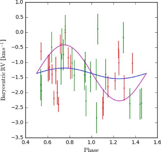
The 21 CORALIE RVs (green) and 20 TRES RVs (red) obtained for WASP-167/KELT-13. The blue line shows the best-fitting semi-amplitude, which we do not regard as reliable. The magenta line shows the RV amplitude for a planet mass of 8 MJup, which we regard as a conservative upper limit.
Attempting to fit for a second planet does not properly explain the scatter, but does significantly change the semi-amplitude fitted to the first planet. For this reason we do not regard the fitted semi-amplitude as a reliable measure of the planet's mass, but instead report an upper limit of 8 MJup, which we regard as conservative but sufficient to demonstrate that the transiting body has a planetary mass. We are continuing to monitor the system in order to discover the cause of the scatter. The parameters obtained in this analysis are given in Table 3.
The TRAPPIST observations of the eclipse (of the planet by the star) produced no detection, with an upper limit of 1100 ppm. Given the stellar and planetary radii (Table 3) this implies that the heated face of the planet must be cooler than 3750 K. The fitted system parameters imply a planet temperature of Teql = 2330 ± 65 K, and thus the non-detection of the eclipse is consistent with the planetary hypothesis.
5 DOPPLER TOMOGRAPHY
We obtained 17 spectra with the ESO 3.6-m/HARPS spectrograph through a transit on the night of 2016 March 1. We also observed the same transit photometrically using TRAPPIST (see light curve r in Fig. 2, Table 1). The standard HARPS Data Reduction Software produces a cross-correlation function (CCF) correlated over a window of ±300 km s−1 (as described in Baranne et al. 1996; Pepe et al. 2002). The CCFs were created using a mask matching a G2 spectral type, containing zeroes at the positions of absorption lines and ones in the continuum.
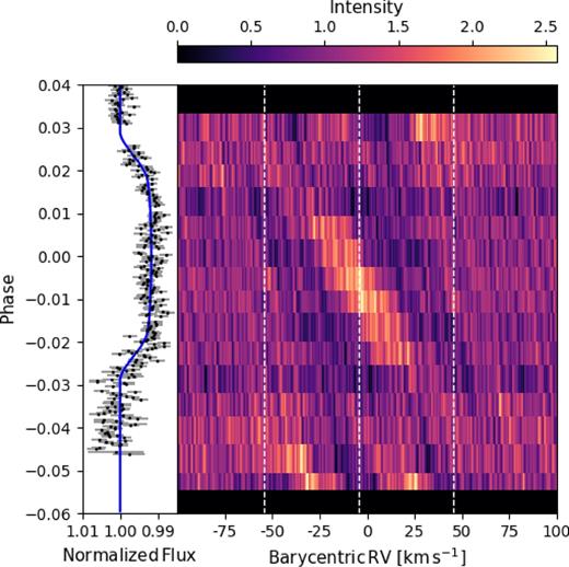
We display the resulting CCFs as a function of the planet's orbital phase in Fig. 4, where phase 0 is mid-transit. In producing this plot, we have first subtracted the invariant part of the CCF profile. We do this by constructing a ‘minimum CCF’, which at each wavelength has the lowest value from the range of phases.
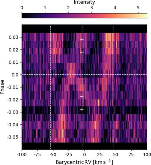
The line profiles through transit. We interpret this as showing prograde-moving stellar pulsations and a retrograde moving planet trace. The white dashed vertical lines mark the positions of the γ velocity of the system and the positions of γ ± v sin i⋆ (i.e. the centre and edges of the stellar line profile). The phase of mid-transit is marked by the white horizontal dashed line. The white + symbols indicate the four transit contact points, calculated using the ephemeris obtained in the analysis in Section 4.
We interpret the CCFs as showing stellar pulsations moving in a prograde direction (moving redward over time). Similar pulsations are seen in the tomograms of WASP-33 (Collier Cameron et al. 2010b; Johnson et al. 2015), which is regarded as a δ-Scuti pulsator (Herrero et al. 2011).
To try to remove the pulsations by separating the features into prograde-moving and retrograde components, we followed the method of Johnson et al. (2015), adopted for WASP-33, by Fourier transforming the CCFs, such that the prograde and retrograde components appear in different quadrants in frequency space.
This separation technique will not be perfect, and we expect some residual contamination from the pulsations. We thus experimented with which data to include. We found that we get the best separation of the components and thus the clearest planetary signal if we do not include in the Fourier transform the last two spectra. These were in any case obtained outside the transit and so cannot contain information about a planet. It is thus valid to try Fourier transforms both with and without these two, in order to see which better separates the pulsations and leaves the clearest planet trace.
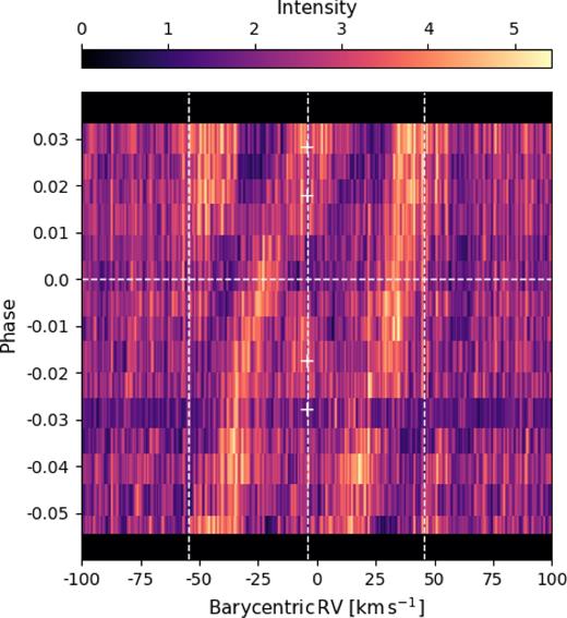
Fig. 5 shows the Fourier-transformed data, where the feature running from bottom-left to top-right can be attributed to the pulsations. We thus applied the filter used by Johnson et al. (2015), which contained zeroes in the quadrants containing the prograde pulsation signal and unity in the quadrants containing the retrograde signal, with a Hann function bridging the discontinuity.
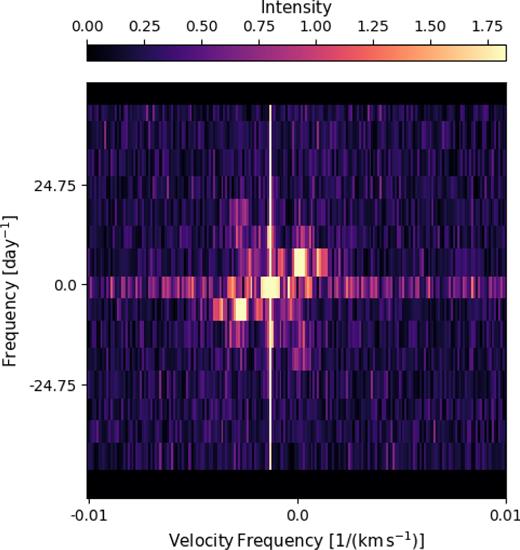
The Fourier transform of the line profiles. The stellar pulsations are seen as the diagonal feature from bottom-left to top-right. The weaker diagonal feature running bottom-right to top-left is produced by the planet.
We then Fourier transform the masked data back into phase versus velocity and display that in Fig. 6. This shows an apparent retrograde trace, which we attribute to the shadow of a planet. This is again similar to what is seen in WASP-33 (Johnson et al. 2015).
The spectral profiles through transit after removing the stellar pulsations via Fourier filtering. The planet trace is then readily seen moving in a retrograde direction. The left-hand panel shows the simultaneous TRAPPIST photometry of the transit.
The planet's Doppler shadow seems to disappear towards the end of the transit (see Fig. 6). It is likely that it has been reduced during the filtering process, as a result of imperfect separation of the planetary and stellar-pulsation signals. This might have some effect on fitting the alignment angle λ, which depends on the slope of the Doppler shadow, but should have less effect on the other fitted quantities.
In order to parametrize the planet's orbit, we then fitted the CCFs through transit, in a manner similar to the methods in Brown et al. (2017). Since we had subtracted the ‘minimum CCF’ above, we first add that back in to the filtered CCFs in order to reintroduce the stellar line profile, which is a key feature for constraining the value of v sin i⋆.
The parameters that define the shape of the CCF line profile are the projected spin–orbit misalignment angle λ, the stellar line-profile full width at half-maximum (FWHM), the FWHM of the line perturbation due to the planet v FWHM, the stellar γ-velocity and v sin i⋆. These parameters were fitted using an MCMC fitting algorithm which assumes a Gaussian shape for the line perturbation caused by the planet. Both v sin i⋆ and v FWHM have two data constraints, one from the shape of the line-broadening profile, and one from the slope of the trajectory of the bump across the line profile (given knowledge of λ). The value of v sin i⋆ obtained in the spectral analysis was used as a prior in the fit. Initial values for the stellar line FWHM and the γ-velocity were obtained by fitting a Gaussian profile to the CCFs. The λ angle and v FWHM were given no prior. Details of the fitting algorithm are given in Collier Cameron et al. (2010a), and the resulting system parameters are listed in Table 3.
Lastly, in Fig. 7 we show the pulsations without the planet trace, obtained by filtering to leave only the prograde quadrants, and then transforming back into velocity space.
The spectral profiles through transit after removing the planet shadow via Fourier filtering. The stellar pulsations are seen moving in a prograde direction.
6 EVOLUTIONARY STATUS
We then used MINESweeper, a newly developed Bayesian approach to determining stellar parameters using the MIST stellar evolution models (Choi et al. 2016). Examples of the use of MINESweeper in determining stellar parameters are shown in Rodriguez et al. (2017a,b). We model the available BT, VT photometry from Tycho-2, J, H, Ks from 2MASS, and WISE W1-3 photometry. We also include in the likelihood calculation the measured parameters from the spectroscopic analysis (Teff = 6900 ± 150 K and [Fe/H] = −0.04 ± 0.18), as well as the Gaia DR1 parallax [π = 2.28 ± 0.62 mas; Gaia Collaboration et al. (2016b,a)] and the fitted transit stellar density (0.28 ± 0.02 ρ⊙). We applied non-informative priors on all parameters within the MIST grid of stellar evolution models, and a non-informative prior on extinction (AV) between 0 and 2.0 mag. Our final parameters are determined from the value at the highest posterior probability for each parameter, and the errors are based on the marginalized inner-68th percentile range. These are given in Table 4.
Stellar parameters obtained for WASP-167/KELT-13 in the SED analysis (see Section 6).
| Parameter (unit) | Value |
|---|---|
| MINESweeper: | |
| Age (Gyr) | 1.29|$^{+0.36}_{-0.27}$| |
| M* (M⊙) | 1.518|$^{+0.069}_{-0.087}$| |
| R* (R⊙) | 1.756|$^{+0.067}_{0.057}$| |
| log L* (L⊙) | 0.835|$^{+0.040}_{-0.034}$| |
| Teff (K) | 7043|$^{+89}_{-68}$| |
| log g* | 4.131|$^{+0.018}_{-0.028}$| |
| [Fe/H]surface | |$-0.01^{+0.17}_{-0.10}$| |
| [Fe/H]init | |$-0.04^{+0.16}_{-0.09}$| |
| Distance (pc) | 381|$^{+15}_{-13}$| |
| AV (mag) | 0.044|$^{+0.057}_{-0.025}$| |
| bagemass: | |
| Age (Gyr) | 1.56 ± 0.40 |
| M* (M⊙) | 1.49 ± 0.09 |
For comparison, we also use the open source software bagemass,1 which uses the Bayesian method described by Maxted, Serenelli & Southworth (2015), to estimate the stellar age and mass. The models used in bagemass were calculated using the garstec stellar evolution code (Weiss & Schlattl 2008). We use the grid of stellar models in bagemass and use the same temperature, metallicity and density constraints as for the MINESweeper calculation. We also apply a luminosity constraint of log LT = 1.00|$^{+0.28}_{-0.22}$|, which was derived using the Gaia parallax and the total line-of-sight reddening as determined by Schlafly & Finkbeiner (2011) and Maxted et al. (2014) [E(B−V) = 0.051 ± 0.034]. The resulting age and mass values are in Table 4. Both values are compatible with those from MINESweeper. The best-fitting stellar evolution tracks and isochrones are shown in Fig. 8.
![The best-fitting evolutionary tracks and isochrones of WASP-167/KELT-13 obtained using bagemass. Dotted blue line: ZAMS at best fit [Fe/H]. Green dashed lines: evolutionary track for the best fit [Fe/H] and mass, plus 1σ bounds. Red lines: isochrone for the best fit [Fe/H] and age, plus 1σ bounds.](https://oup.silverchair-cdn.com/oup/backfile/Content_public/Journal/mnras/471/3/10.1093_mnras_stx1729/1/m_stx1729fig8.jpeg?Expires=1750230716&Signature=1S0zNdVVVImwx~q3s8TjBZPR8KvMQtLYeqxzpuMUDymJNfoZWBjK9FNiQZgVrWF-OXWDsbQC~FbjBDt~8PX7gQPNx6DUKHRV91QIWbgfLl4w1pW9y8d9vT8bJq5ufb5NEvJA50iX0ST7jdM1tbIJazJU1UlrTqWcg9UDCvO~YoZJOxHKoOgNPTJfFRi-J2iLrf9B6QbtdVL-ip~N7I6U4~i6adg2r5PbQqpNJnHY1EGhrBBPwqMcfbrey6Tu1vt0ZI8lPFx0VeQBlvQ0bfLiB-fn37N6HmHxxrIkhOlOHR9EA9W6crqP1W8ZRTh1pAT2KyB4NsCKtJ5U4LXgy561Yg__&Key-Pair-Id=APKAIE5G5CRDK6RD3PGA)
The best-fitting evolutionary tracks and isochrones of WASP-167/KELT-13 obtained using bagemass. Dotted blue line: ZAMS at best fit [Fe/H]. Green dashed lines: evolutionary track for the best fit [Fe/H] and mass, plus 1σ bounds. Red lines: isochrone for the best fit [Fe/H] and age, plus 1σ bounds.
7 DISCUSSION
7.1 Stellar rotation rate and tidal interaction
As an F1V star with Teff = 6900 ± 150 K, WASP-167/KELT-13 is among the hottest stars known to host a transiting hot Jupiter. Others include WASP-33 (Collier Cameron et al. 2010b), Kepler-13 (Shporer et al. 2011, 2014), KELT-17 (Zhou et al. 2016), HAT-P-57 (Hartman et al. 2015) and KELT-9 (Gaudi et al. 2017).
In addition, WASP-167/KELT-13 appears to be one of the most rapidly rotating stars known to host a hot Jupiter, and one of the few with a stellar rotation period shorter than the planet's orbit. The measured v sin i⋆ of 49.94 ± 0.04 km s−1 and the fitted radius of 1.79 ± 0.05 R⊙ imply a rotation period of Prot<1.81 d, which compares with the planet's orbital period of 2.02 d.
Thus WASP-167/KELT-13 joins WASP-33 (Porb = 1.22 d; Prot < 0.79 d, Collier Cameron et al. 2010b), KELT-7 (Porb = 2.7 d, Prot < 1.32 d, Bieryla et al. 2015) and CoRoT-11b (Porb = 3.0 d; Prot < 1.73 d, Gandolfi et al. 2010) in having a hot Jupiter in a <3-d orbit and an even shorter rotation rate. See also Crouzet et al. (2017) for a discussion of other systems with Prot < Porb but with longer period orbits.
The tidal interaction will be different in such systems compared to the more-usual Prot > Porb. In most hot Jupiters, the tidal interaction is expected to drain angular momentum from the orbit, leading to tidal decay of the orbital period (e.g. Levrard, Winisdoerffer & Chabrier 2009). This would be reversed, however, for systems with Prot < Porb, and with the planet in a prograde orbit (such as KELT-7b and CoRoT-11b), thus leading to a different dynamical history.
If, though, Prot < Porb and with the planet in a retrograde orbit, such as WASP-167b/KELT-13b or WASP-33b, tidal infall would again be expected. McQuillan et al. (2013) analysed Kepler detections and found a dearth of close-in planets around fast rotators, saying that only stars with rotation periods longer than 5–10 d have planets with periods shorter than 3 d. Teitler & Königl (2014) then attributed this to the destruction of close-in planets, with the result of spinning up the star. While WASP-167/KELT-13 and the others just named are examples of systems with Prot < Porb they are undoubtedly rare and their dynamics deserves further investigation.
7.2 The retrograde orbit
The planet WASP-167b/KELT-13b has a radius of 1.6 RJup and is thus inflated, though not exceptionally so. This is in line with WASP-33b, which has a 1.5 RJup radius, and is expected for a hot Jupiter orbiting a hot star, given that a relation between inflated radii and stellar irradiation is now well established (e.g. Demory & Seager 2011; Enoch, Collier Cameron & Horne 2012; Hartman et al. 2016). We should, though, warn of a selection effect against observing non-inflated planets around relatively large A/F stars, in that the transits would be shallower and may escape detection in WASP-like surveys.
Crouzet et al. (2017) list six planets with measured sky-projected obliquity angles (λ) that transit host stars hotter than 6700 K (these are XO-6b, CoRoT-3b, KELT-7b, KOI-12b, WASP-33b and Kepler-13Ab). Of these, five seem to be misaligned but only moderately so, having non-zero λ values with |λ| typically 10–40°. HAT-P-57b (Hartman et al. 2015) is also likely to be moderately misaligned with 27° < λ < 58°. The KELT-9b system (Gaudi et al. 2017) is the most recently discovered example, with the hottest star known to host a transiting planet (∼10 000 K) and the planet itself on a near-polar orbit (λ ∼ –85°). WASP-33b is the exception in the list of Crouzet et al. (2017), being highly retrograde with λ = −109° ± 1° (Collier Cameron et al. 2010b), and the same is now seen in WASP-167b/KELT-13b with λ = −165° ± 5°.
As has been widely discussed (e.g. Albrecht et al. 2012; Crida & Batygin 2014; Fielding et al. 2015; Li & Winn 2016), stars hotter than 6100 K host hot Jupiters with a large range of obliquities, whereas cooler stars tend to have planets in aligned orbits (see e.g. fig. 8 of Crouzet et al. 2017). The suggestion is that hotter stars are less effective at tidally damping a planet's obliquity, perhaps owing to their relatively small convective envelopes (e.g. Winn et al. 2010). The discovery of WASP-167b/KELT-13b now reinforces this trend.
7.3 Stellar pulsations
WASP-167/KELT-13 is one of a growing number of hot-Jupiter hosts that have shown non-radial pulsations. The first was WASP-33b (Collier Cameron et al. 2010b), which shows δ-Scuti pulsations with a dominant period near 21 cycles/day (86 mins) and an amplitude of several mmag (Kovács et al. 2013; von Essen et al. 2014). Further, Herrero et al. (2011) noted that one of the pulsation frequencies was very near 26 times the orbital frequency of the planet, which suggests that the planet might be exciting the pulsations.
HAT-P-2b is an eccentric massive planet (8 MJup, e ∼ 0.5) in a 5-d orbit. de Wit et al. (2017) detect pulsations in Spitzer light curves of HAT-P-2b, at a level of 40 ppm, much lower than in WASP-33b, but at a similar time-scale of ∼87 mins. Owing to the commensurability between the pulsation and orbital frequencies, de Wit et al. (2017) again suggest that the planet is exciting the pulsations.
A third example is WASP-118, which shows pulsations at a time-scale of ∼1.9 d and an amplitude of ∼200 ppm in K2 observations (Močnik et al. 2017). Another is HAT-P-56, a γ-Dor pulsator with a primary pulsation period of 1.644 ± 0.03 d, which were also seen in K2 observations (Huang et al. 2015).
It is worth noting that both planets WASP-33b and WASP-167b/KELT-13b have retrograde orbits, whereas that of HAT-P-2b is highly eccentric, which may be relevant to the excitation of the pulsations.
In WASP-167/KELT-13, judging from Fig. 4, the pulsations appear to have a time-scale of ∼4 h, though with limited data we cannot be more precise. The pulsations in WASP-167/KELT-13 have a longer time-scale than in WASP-33 and HAT-P-2 and are near the borderline between δ-Scuti and γ-Dor behaviour, and so we are unsure which class to assign the star to.
It may be that the pulsations are contributing to the scatter in the RV measurements seen in Fig. 3. Indeed, de Wit et al. (2017) attribute radial-velocity scatter in HAT-P-2 to the pulsations. Hay et al. (2016) also report excess RV scatter in WASP-118.
We have looked for the pulsations in the WASP and KELT photometry, but do not detect any signal, with an upper limit of 0.5 mmag. However, we caution that the WASP data are not particularly suitable for searching for periodicities of 4–8 h. This is comparable to the length of observation on each night, and is thus the time-scale of greatest red noise in WASP data. For this reason, WASP data are processed to reduce sinusoidal-like variations on such time-scales (Collier Cameron et al. 2006). Similar considerations apply to the KELT data, which in any case have lower photometric precision. The higher quality follow-up photometry was aimed at observing the transits, before we were aware of the presence of pulsations, and none of the observations are long enough to search for the pulsations.
It is also possible that the particular mode of pulsations can lead to scatter in the RV measurements but smaller photometric variations owing to geometric cancellation. Axisymmetric non-radial pulsations of order l ≥ 3 are subject to partial geometric cancellation: the greater the value of l, the larger the cancellation effect, and odd-numbered modes are near invisible in intensity measurements (Aerts, Christensen-Dalsgaard & Kurtz 2010).
Acknowledgements
WASP-South is hosted by the South African Astronomical Observatory and we are grateful for their ongoing support and assistance. Funding for WASP comes from consortium universities and from the UK's Science and Technology Facilities Council. The Euler Swiss telescope is supported by the Swiss National Science Foundation. TRAPPIST is funded by the Belgian Fund for Scientific Research (Fond National de la Recherche Scientifique, FNRS) under the grant FRFC 2.5.594.09.F, with the participation of the Swiss National Science Foundation (SNF). M. Gillon and E. Jehin are FNRS Research Associates. We acknowledge use of the ESO 3.6-m/HARPS under program 096.C-0762. L. Delrez acknowledges support from the Gruber Foundation Fellowship.
Work performed by PAC was supported by NASA grant NNX13AI46G. DJS and BSG were partially supported by NSF CAREER Grant AST-1056524. SV is supported by the National Science Foundation Graduate Research Fellowship under Grant No. DGE-1343012. Work performed by JER was supported by the Harvard Future Faculty Leaders Postdoctoral fellowship.
REFERENCES
