Formation of solar system analogues – I. Looking for initial conditions through a population synthesis analysis

Ronco, M. P.; Guilera, O. M.; de Elía, G. C.

doi:10.1093/mnras/stx1746

Abstract

Population synthesis models of planetary systems developed during the last ∼15 yr could reproduce several of the observables of the exoplanet population, and also allowed us to constrain planetary formation models. We present our planet formation model, which calculates the evolution of a planetary system during the gaseous phase. The code incorporates relevant physical phenomena for the formation of a planetary system, like photoevaporation, planet migration, gas accretion, water delivery in embryos and planetesimals, a detailed study of the orbital evolution of the planetesimal population, and the treatment of the fusion between embryos, considering their atmospheres. The main goal of this work, unlike other works of planetary population synthesis, is to find suitable scenarios and physical parameters of the disc to form Solar system analogues. We are specially interested in the final planet distributions, and in the final surface density, eccentricity and inclination profiles for the planetesimal population. These final distributions will be used as initial conditions for N-body simulations to study the post-oligarchic formation in a second work. We then consider different formation scenarios, with different planetesimal sizes and different type I migration rates. We find that Solar system analogues are favoured in massive discs, with low type I migration rates, and small planetesimal sizes. Besides, those rocky planets within their habitables zones are dry when discs dissipate. At last, the final configurations of Solar system analogues include information about the mass and semimajor axis of the planets, water contents, and the properties of the planetesimal remnants.

methods: numerical, planets and satellites: formation, protoplanetary discs

1 INTRODUCTION

For a long time, the study of planetary systems was restricted to our own Solar system. However, this situation had a drastic change since the discovery of the first exoplanet orbiting a sun-like star, 51 Peg b, in 1995 (Mayor & Queloz 1995). 51 Peg b, named as Dimidium by the International Astronomical Union in December 2015, is what we know now as a hot-Jupiter, a gas giant planet orbiting very close to its parent star. Since this discovery, the observational field of extrasolar planet search had an explosion, leading to numerous additional discoveries of planets orbiting other stars. Up to date, 3610 exoplanets that show a wide range of masses, orbits and compositional properties have been discovered orbiting near stars (http://exoplanet.eu/, Schneider et al. 2011). Some of them are hot and warm Jupiters, Jupiter-analogues, giant planets at wide orbits, hot-Neptunes, super-Earths, etc. Moreover, much of these planets form part of about 610 multiple planet systems. These systems represent the final stage of a series of complex processes, where a protoplanetary disc evolves into a planetary system, with a few planets and probably, reservoirs of small bodies, like in our Solar system. These discoveries also triggered theoretical studies about the formation and evolution of planetary systems. During more than a decade, several models of planet formation have been developed to study the formation of planetary systems and population synthesis with the aim to reproduce the main properties of the observational sample of exoplanets, and to get a better understanding of the main processes of planetary formation (see Benz et al. 2014, for a detailed review).

The first models of planetary population synthesis were developed in the pioneer works of Ida & Lin (2004a,b, 2005, 2008a,b). In these works, the authors could numerically reproduce several of the main observed properties of the populations of exoplanets, specially the mass versus semimajor-axis diagram (M-a diagram). Thommes, Matsumura & Rasio (2008) studied the formation of planetary systems with an hybrid model, including N-body interaction between embryos, with the aim to link a mature planetary system with the properties of the protoplanetary disc where it was born. They found that Solar system analogues are not common. These systems can form when the time-scale for the formation of the giant planets is similar to the time-scale of the disc dissipation, undergoing only modest type I migration, and for massive discs. Otherwise, Miguel, Guilera & Brunini (2011) found that Solar system analogues might not be so rare in the solar neighbourhood, where the formation of such systems could be favoured by massive discs, and where there is not a large accumulation of solids in the inner region. In other case, very slow type I migration is needed to form giant planets. However, Miguel et al. (2011) did not analyse the post-oligarchic growth and long-term evolution of the planetary systems and adopted a different definition for Solar system analogues. More recently, Alibert et al. (2013) introduced a distribution of embryos calculating the gravitational interactions between them in their planetary population synthesis model (Alibert et al. 2005; Mordasini et al. 2009; Fortier et al. 2013), which previously calculates planetary population synthesis but considering only one planet per disc. These authors also showed that the main observed properties of the exoplanets M-a diagram can be reproduced, focusing in low-mass planets. Then, Pfyffer et al. (2015) used the results of Alibert et al. (2013) as initial conditions to calculate the long-term evolution of the planetary population synthesis but only considering the distribution of embryos and without including the remnant of planetesimal distributions. They found that the M-a diagram does not experience significantly changes due to the long-term evolution of the systems, but that the eccentricity distributions of such systems do not match the observed ones in the known exoplanets. Moreover, Ida, Lin & Nagasawa (2013) also introduced gravitational interactions between embryos in their planetary population synthesis model using a Monte Carlo approach (not calculating N-body integrations) founding that the observed planetary mass-eccentricity and M-a diagrams can be reproduced. However, in most of the cases, the evolution of the planetesimal population is treated in a simplified way and is not taken into account in the calculations of the long-term evolution of the systems.

On the other hand, several works study the formation of terrestrial planets in the post-oligarchic growth regime and the water delivery via purely N-body calculations considering a distribution of embryos and planetesimals after the dissipation of the primordial nebula (Chambers 2001; Raymond, Quinn & Lunine 2004, 2005, 2006; Raymond et al. 2009; O'Brien, Morbidelli & Levison 2006; O'Brien et al. 2014; Walsh et al. 2011; Ronco & de Elía 2014). In general, the orbital initial conditions for the distributions of embryos and planetesimals are typically selected ad hoc. However, Ronco, de Elía & Guilera (2015) showed that more realistic initial conditions lead to different accretion histories of the planets that remain in the habitable zone compared to the case of ad hoc initial conditions.

The aim of this first work is to improve our model of planet formation during the gaseous phase to obtain accurate initial conditions for the distributions of planets and planetesimals, to perform future high-resolution N-body calculations for the analysis of the formation of terrestrial planets and water delivery in Solar system analogues. To do so, we first include the most relevant physical phenomena that take place in the formation of a planetary system during the gaseous phase. Then, we perform a planetary population synthesis calculation in order to obtain the main properties of the protoplanetary discs that lead to the formation of Solar system analogues. This work is then organized as follow. In Section 2, we describe our planet formation model; in Section 3, we describe the initial conditions for the development of our planetary systems; in Section 4, we show the results; and in Section 5, we discuss the conclusions.

2 DESCRIPTION OF OUR MODEL OF PLANET FORMATION

We have improved a model of planet formation based on previous works (Guilera, Brunini & Benvenuto 2010; Guilera et al. 2011, 2014), which we now called PLANETALP. This code describes the evolution in time of a planetary system during the gaseous phase and incorporates many of the most important physical phenomena for the formation of planetary systems. PLANETALP is a code developed almost entirely in fortran 95/2003 and has the advantage of being programmed in a modular way so as to be able to turn on or turn off the different physical phenomena according to the user's choice.

Our model presents a protoplanetary disc, which is characterized by two components: a gaseous component, evolving due to an α-viscosity driven accretion and photoevaporation processes, and a solid component represented by a planetesimal population being subject to accretion and ejection by the embryos, and radial drift due to gas drag. Besides, the model presents an embryo population which is also part of the solid component of the disc and which grows by accretion of planetesimals, gas, and due to the fusion between them taking into account their atmospheres. The new improvements made in PLANETALP with respect to previous versions of this code (Guilera et al. 2010, 2011, 2014) are described in detail in the next subsections.

2.1 Protoplanetary disc structure

The gaseous component is characterized by the gas surface density Σ_g(R), where R is the radial coordinate in the midplane of the disc, and the planetesimal population is characterized by the planetesimal surface density Σ_p(R). Although our model allows us to include a discrete planetesimal size distribution described by Σ_p(R, r_p), where r_p represents the different sizes of the planetesimals, we will consider in this work only one size of planetesimals for each simulation. Both Σ_g(R) and Σ_p(R) determine the mass distribution along the protoplanetary disc. In this work, as in previous ones (de Elía, Guilera & Brunini 2013; Ronco et al. 2015; Dugaro et al. 2016), we consider the surface density profile suggested by Andrews et al. (2010), who found that the discs observed in the Ophiuchus star-forming region can be represented by

\begin{eqnarray} \Sigma _{{\rm g}}(R) = \Sigma ^{0}_{{\rm g}}\left(\frac{R}{R_{{\rm c}}}\right)^{-\gamma }{\rm e}^{-\left(\frac{R}{R_{{\rm c}}}\right)^{2-\gamma }}, \end{eqnarray}

(1)

where R_c is a characteristic radius of the disc, γ is the exponent that represents the surface density gradient and |$\Sigma _{{\rm g}}^{0}$| is a normalization constant, which is a function of the mass of the disc M_d, R_c and γ, that can be obtained by integrating equation (1) over the total area of the disc. Assuming that the metallicity along the disc is the same as that of the central star, and considering that the dust sediments and coagulates very quickly to form a mid-plane planetesimal disc, is that the planetesimal surface density profile is given by

\begin{eqnarray} \Sigma _{{\rm p}}(R) = \Sigma ^{0}_{{\rm p}}\eta _{{\rm ice}}\left(\frac{R}{R_{{\rm c}}}\right)^{-\gamma }{\rm e}^{-\left(\frac{R}{R_{{\rm c}}}\right)^{2-\gamma }}, \end{eqnarray}

(2)

where |$\Sigma ^{0}_{{\rm p}} = z_0\Sigma ^{0}_{{\rm g}}10^{[{\rm Fe/H}]}$| is a normalization constant, z₀ = 0.0153 is the primordial abundance of heavy elements in the Sun (Lodders, Palme & Gail 2009), [Fe/H] is the stellar metallicity, and η_ice is a parameter that represents an increase in the amount of solid material due to the condensation of water beyond the snowline, given by

\begin{eqnarray} \eta _{{\rm ice}}= \left\lbrace \begin{array}{@{}l@{\quad }l@{}}1 & {\rm if}\, R \ge R_{{\rm ice}}, \\ {\displaystyle\frac{1}{\beta }} & {\rm if}\, R < R_{{\rm ice}}, \end{array}\right. \end{eqnarray}

(3)

where R_ice represents the position in the disc where water condensates, usually at 170° K, and the factor β represents the amount of material condensed. In our Solar system, β usually takes a value of approximately 2 (Lodders 2003; Lodders et al. 2009).

The values of the free parameters involved in the structure of the protoplanetary disc like the mass of the disc M_d, the characteristic radius R_c, the surface density gradient γ and the factor β will be discussed in the next section.

2.1.1 Evolution of the gaseous component

As it was mentioned before, we improved the evolution of the gaseous component considering a viscous accretion disc (Pringle 1981) with photoevaporation.

The evolution in time of the gas surface density is then represented by a diffusion equation

\begin{eqnarray} \frac{\mathrm{\partial} \Sigma _{{\rm g}}}{\mathrm{\partial} t}= \frac{3}{R}\frac{\mathrm{\partial} }{\mathrm{\partial} R} \left[ R^{1/2} \frac{\mathrm{\partial} }{\mathrm{\partial} R} \left( \nu \Sigma _{{\rm g}} R^{1/2} \right) \right] + \dot{\Sigma }_{{\rm w}}(R), \end{eqnarray}

(4)

where ν = αc_sH_g represents the Shakura and Sunyaev viscosity (Shakura & Sunyaev 1973) with α a constant a-dimensional parameter along the disc, c_s the sound speed, H_g the height scale of the disc, and |$\dot{\Sigma }_{{\rm w}}(R)$| the photoevaporation sink term. The sound speed is given by

\begin{eqnarray} c_{{\rm s}}= \sqrt{ \frac{\gamma _{{\rm g}} k_{{\rm B}} {\rm T}}{\mu _{{\rm H}_2} m_{{\rm H}_2}} }, \end{eqnarray}

(5)

where γ_g = 5/3, k_B is the Boltzmann constant, and |$\mu _{{\rm H}_2}$| and |$m_{{\rm H}_2}$| are the molecular weight and mass of molecular hydrogen, respectively. Following Hayashi (1981) and Ida & Lin (2004a), we consider a temperature profile given by

\begin{eqnarray} {\rm {\it T}}= 280 \left( \frac{R}{1\ {\rm au}} \right)^{-1/2} \ {\rm K}, \end{eqnarray}

(6)

where, according to this, R_ice is defined as 2.7 au. Finally, the height scale of the disc is |$H_{{\rm g}} = \sqrt{2}c_{{\rm s}}/\Omega _{{\rm k}}$|⁠, where Ω_k is the Keplerian frequency. It is important to note that we are considering a flare disc, where H_g ∝ R^5/4.

Finally, |$\dot{\Sigma }_{{\rm w}}(R)$| represents the photoevaporation rate. There are different photoevaporation regimes, and they depend on which is the source that emits irradiation. This source could be the central star (Dullemond et al. 2007; D'Angelo & Marzari 2012), or external stars that irradiate the environment in where the disc forms (Veras & Armitage 2004). If our sun was formed in a densely populated environment, the high stellar density could lead to encounters with stars that could affect and modify the size of the disc by photoevaporation (see Moro-Martín et al. 2008, and references therein). However, since up to date the environment in which our Solar system was formed is still under discussion, and due to the fact that photoevaporation by the central star is, probably, the most important photoevaporation regime that affects the planet formation region, we only consider this case. Thus, following the model of Dullemond et al. (2007), also adopted by D'Angelo & Marzari (2012), |$\dot{\Sigma }_{{\rm w}}(R)$| is given by

\begin{eqnarray} \dot{\Sigma }_{{\rm w}}(R) = \left\lbrace \begin{array}{@{}l@{\quad }l@{}}\dot{\Sigma }^{g}_{{\rm w}}\exp {\left[\displaystyle\frac{1}{2}\left(1-\displaystyle\frac{R_{{\rm g}}}{R}\right)\right]}\left(\displaystyle\frac{R_{{\rm g}}}{R}\right)^2 & {\rm if}\, R \le R_{{\rm g}}, \\ \dot{\Sigma }^{g}_{{\rm w}}\left(\displaystyle\frac{R_{{\rm g}}}{R}\right)^{5/2} & {\rm if} \, R > R_{{\rm g}}, \end{array}\right. \end{eqnarray}

(7)

where R_g is the radius of the gas surface layer at which the sound speed equals the local Keplerian velocity, and beyond which the gas is disengaged from the disc. The photoevaporation rate at R_g is represented by |$\dot{\Sigma }^{g}_{{\rm w}}$| and is given by

\begin{eqnarray} \dot{\Sigma }^{g}_{{\rm w}} = 1.16 \times 10^{-11}f^{0.5}_{41}\left(\frac{1{\rm au}}{R_{{\rm g}}}\right)^{1.5}\frac{{\rm M}_{\odot }}{{\rm au}^{2}{\rm yr}}, \end{eqnarray}

(8)

where f₄₁ is the rate of EUV ionizing photons emitted by the star in units of 10⁴¹s⁻¹. It is worth noting that R_g is usually taken to be 10 au for a solar-mass star.

Equation (4) is solved on a disc defined between 0.1 and 1000 au, using 5000 radial bins logarithmically equally spaced. It is worth remarking that we consider that the disc is dissipated when the mass of gas becomes lower than 10⁻⁶ M_⊙.

2.1.2 Evolution of the planetesimal population

In our model, the planetesimal population evolves by the drift of planetesimals due to the nebular gas including the Epstein, Stokes and quadratic regimes, and the accretion and ejection by the embryos. We also consider that the evolution of the eccentricities and inclinations of the planetesimals are due to two principal processes: the embryo gravitational excitation (Ohtsuki, Stewart & Ida 2002) and the damping due to the nebular gas drag (Rafikov 2004; Chambers 2008). The treatment of these processes is described in detail in Guilera et al. (2014). Then, the evolution in time of the planetesimal surface density is modelled with a continuity equation given by

\begin{eqnarray} \frac{\mathrm{\partial} \Sigma _{{\rm p}}(R)}{\mathrm{\partial} t} - \frac{1}{R} \frac{\mathrm{\partial} }{\mathrm{\partial} R} \left[ Rv_{{\rm mig}}(R)\Sigma _{{\rm p}}(R) \right] = \dot{\Sigma }^{{\rm tot}}_{{\rm p}}(R), \end{eqnarray}

(9)

\begin{eqnarray} \dot{\Sigma }^{{\rm tot}}_{{\rm p}}(R) = \dot{\Sigma }^{{\rm ac}}_{{\rm p}}(R) + \dot{\Sigma }^{{\rm sc}}_{{\rm p}}(R) + \dot{\Sigma }^{{\rm ej}}_{{\rm p}}(R), \end{eqnarray}

(10)

where v_mig is the planetesimal migration velocity and |$\dot{\Sigma }^{{\rm ac}}_{{\rm p}}(R)$|⁠, |$\dot{\Sigma }^{{\rm sc}}_{{\rm p}}(R)$| and |$\dot{\Sigma }^{{\rm ej}}_{{\rm p}}(R)$| represent the sink terms due to the accretion by the embryos, due to the probability of scattered planetesimals and due to the ejection of planetesimals with high eccentricities, respectively. In this work, we incorporate two different ejection rates of planetesimals that play different roles. It is important to remark that the ejected planetesimals are directly removed from the planetary system and are not relocated in a different orbit. The first one, |$\dot{\Sigma }^{{\rm sc}}_{{\rm p}}(R)$|⁠, considers the ejection rate of planetesimals proposed by Ida & Lin (2004a) and also adopted by Alibert et al. (2005), which takes into account the probability of planetesimal scattering rather than collisions during close encounters, and is

\begin{eqnarray} \dot{\Sigma }^{{\rm sc}}_{{\rm p}}(R) = \frac{1}{4}\left(\frac{a_{{\rm P}}M_{{\rm P}}}{M_\star \tilde{R}_{{\rm C}}}\right)^{2}\dot{\Sigma }^{{\rm ac}}_{{\rm p}}(R), \end{eqnarray}

(11)

where a_P and M_P are the semimajor-axis and the total mass of the planet, respectively, and |$\tilde{R}_{{\rm C}}$| is the planet's enhanced radius (see the next section). The second one, |$\dot{\Sigma }^{{\rm ej}}_{{\rm p}}(R)$|⁠, considers the ejection of planetesimals that reach values of the eccentricity higher than 0.99. As the gas disc evolves, the gas surface density decreases, and because of this, the eccentricities of the planetesimals that are in the vicinity of the massive planets are no longer efficiently damped by the gas, and therefore, they increase considerably. At this time, |$\dot{\Sigma }^{{\rm ej}}_{{\rm p}}(R)$| becomes effective. As in Laakso, Rantala & Kaasalainen (2006), we consider that the probability of a particle to be ejected per unit time is constant. This implies that |$\dot{\Sigma }^{{\rm ej}}_{{\rm p}}= -\rho \Sigma _{{\rm p}}$|⁠, where we adopt ad hoc values of ρ between 0.001 and 0.01 yr⁻¹. These values represent the ejection of the 0.1 per cent and 1 per cent, respectively, of the available planetesimals in each radial bin around the planet at each time-step, finding no differences in the final results.

We use a full implicit upwind-downwind mix method to solve equation (9), considering density equal to zero as boundary conditions. We do not allow changes greater than 10 per cent for the planetesimal surface density profile in each time-step and in each radial bin.

2.2 Growth and orbital evolution of the protoplanetary embryos

At the beginning of our model, an embryo population is immersed in the protoplanetary disc. Here, we describe the details on the embryos growth and orbital evolution.

2.2.1 Solid accretion by the embryos

The embryos grow within the oligarchic regime, and the accretion of planetesimals is well described by the particle in a box approximation (Inaba et al. 2001):

\begin{eqnarray} \frac{{\rm d}M_{{\rm C}}}{{\rm d}t} = \frac{2\pi \Sigma _{{\rm p}}({a_{{\rm P}}})R^{2}_{{\rm H}}}{P}P_{{\rm coll}}, \end{eqnarray}

(12)

where M_C is the mass of the core, Σ_p(a_P) is the planetesimal surface density at the planet location, R_H is the Hill radius, P is the orbital period and P_coll is the collision probability. P_coll is a function of the enhanced radius |$\tilde{R}_{{\rm C}}$|⁠, the Hill radius of the planet and the relative velocity of planetesimals, |$P_{{\rm coll}} = P_{{\rm coll}}(\tilde{R}_{{\rm C}},R_{{\rm H}},v_{{\rm rel}})$|⁠. The fact that P_coll is function of the enhanced radius |$\tilde{R}_{{\rm C}}$| instead of the core radius R_C is due to the fact that we are considering the drag force experienced by planetesimals when entering the planetary envelope. Here, |$v_{{\rm rel}}= \sqrt{5e^{2}/8+i^{2}/2}\ v_{{\rm k}}$|⁠, where e represents the eccentricity, i the inclination and v_k the Keplerian velocity of the planetesimal population (see Guilera et al. 2010 for further details). It is worth remarking that the embryos evolve in circular and coplanar orbits during all the simulation.

In contrast to our previous works, we do not solve the equations of transport and structure for the envelope; thus, we calculate |$\tilde{R}_{{\rm C}}$| following the works of Ormel & Kobayashi (2012) and Chambers (2014) as

\begin{eqnarray} \tilde{R}_{{\rm C}}= \left\lbrace \begin{array}{@{}l@{\quad }l@{}}\displaystyle\frac{R_{\rm B}}{1 + \displaystyle\frac{2W(\sigma _{{\rm crit}}-1) + \ln (\sigma _{{\rm crit}})}{\gamma _{{\rm g}}}},& {\rm if}\ \sigma _{{\rm crit}} < \sigma _t, \\ \displaystyle\frac{R_{\rm B}}{\displaystyle\frac{R_{\rm B}}{R_t} + \displaystyle\frac{4}{\gamma _{{\rm g}}} (4W)^{1/3} \left(\sigma _{{\rm crit}}^{1/3} - \sigma _t^{1/3}\right)},& {\rm if}\ \sigma _{{\rm crit}} > \sigma _t, \end{array}\right. \end{eqnarray}

(13)

where

\begin{align} \frac{R_{\rm B}}{R_t} = 1 + \frac{2W(\sigma _t - 1) + \ln (\sigma _t)}{\gamma _{{\rm g}}}, \end{align}

(14)

\begin{align} W = \frac{3\kappa _e L P_{{\rm neb}}}{64 \pi \sigma _B G M_{{\rm C}} T_{{\rm neb}}^4}, \end{align}

(15)

\begin{align} \sigma _t = \frac{1}{5W}, \end{align}

(16)

\begin{align} \sigma _{{\rm crit}} = \frac{\rho _{{\rm p}}r_{{\rm p}}v_{{\rm rel}}^2}{3GM_{{\rm C}}\rho _{{\rm neb}}}, \end{align}

(17)

\begin{align} L = \left(\frac{GM_{{\rm C}}}{R_{{\rm C}}}\right) \frac{{\rm d}M_{{\rm C}}}{{\rm d}t}, \end{align}

(18)

\begin{align} R_{\rm B} = \frac{GM_{{\rm C}}}{c_{{\rm s}}^2}. \end{align}

(19)

In the previous equations, R_B is the Bondi radius of the planet, L is the luminosity generated due to the accretion of planetesimals, G is the universal gravitational constant, R_C is the radius of the core, ρ_p is the planetesimal density, σ_B is the Stefan-Boltzmann constant, κ_e = 0.01 cm²g⁻¹ the envelope opacity, and P_neb, T_neb, ρ_neb the local pressure, temperature and density of the nebular gas, respectively.

2.2.2 Gas accretion by the embryos

As the embryos grow, they are able to retain a gaseous envelope that is capable to maintain hydrostatic equilibrium. Initially, the gas accretion rate is much lower than the planetesimal accretion rate; thus, the core of the embryo grows faster than the corresponding envelope. However, when the core of the planet reaches a critical mass, the gas accretion begins to be substantial. Following Ida & Lin (2004a), the critical mass is given by

\begin{eqnarray} M_{{\rm crit}} \sim 10\left(\frac{\dot{M}_{{\rm C}}}{10^{-6}{\rm M}_{\hbox{$\oplus $}} {\rm yr}^{-1}}\right)^{0.25}{\rm M}_{\hbox{$\oplus $}}, \end{eqnarray}

(20)

where, as we have already seen, |$\dot{M}_{{\rm C}}$| is the planetesimal accretion rate. The gas accretion rate can be estimated by

\begin{eqnarray} \dot{M}_{{\rm KH}} = \frac{{\rm d}M_{{\rm g}}}{{\rm d}t} = \frac{M_{{\rm P}}}{\tau _{{\rm g}}} \end{eqnarray}

(21)

where M_P is the total mass of the planet and τ_g is the characteristic Kelvin–Helmholtz growth time-scale of the envelope. According to the results of the giant planet formation model of Guilera et al. (2010, 2014), and following the prescription of Ida & Lin (2004a), τ_g is fitted by

\begin{eqnarray} \tau _{{\rm g}} = 8.35\times 10^{10}(M_{{\rm P}}/{\rm M}_{\hbox{$\oplus $}})^{-3.65}{\rm yr}. \end{eqnarray}

(22)

Note that, unlike Miguel et al. (2011), we found a different exponent in the dependence with the mass of the planet of τ_g. These authors found an exponent of −4.89. This difference is due to the fact that the fit on the gas accretion has been done for slightly different giant planet formation models.¹

It is important to remark that |$\dot{M}_{{\rm KH}}$| is valid as long as it is less than the maximum rate at which the gas can be delivered by the disc on to the planet, which, following (Mordasini et al. 2009), is

\begin{eqnarray} \dot{M}_{{\rm disc}} = \frac{{\rm d}M_{{\rm g}}}{{\rm d}t} = 3\pi \nu \Sigma _{{\rm g}}(R). \end{eqnarray}

(23)

Thus, we consider that the effective gas accretion rate is

\begin{eqnarray} \frac{{\rm d}M_{{\rm g}}}{{\rm d}t} = {\rm min}[\dot{M}_{{\rm KH}},\dot{M}_{{\rm disc}}]. \end{eqnarray}

(24)

The process of gas accretion by the planet is also limited if the planet is able to open a gap. Through high-resolution hydrodynamical simulations, Tanigawa & Ikoma (2007) found that the gas accretion rate decreases significantly when a planet opens a gap in what they called the ‘gap-limiting’ case. Following this idea, Tanigawa & Ikoma (2007) developed an analytic formula for the accretion rate also adopted by Xiao & Jin (2015):

\begin{eqnarray} \dot{M}_{{\rm GP}} = \frac{{\rm d}M_{{\rm g}}}{{\rm d}t} = \dot{A}\Sigma _{{\rm acc}}, \end{eqnarray}

(25)

where

\begin{eqnarray} \dot{A} = 0.29\left(\frac{H_{{\rm g,P}}}{a_{{\rm P}}}\right)^{-2}\left(\frac{M_{{\rm P}}}{M_{\star }}\right)^{4/3}a^{2}_{{\rm P}}\Omega _{{\rm k,P}} \end{eqnarray}

(26)

with Σ_acc = Σ(x = 2R_H) and,

\begin{eqnarray} \Sigma (x) = \left\lbrace \begin{array}{lr}\Sigma _{{\rm g}}{\rm exp}\left[-\left( \displaystyle\frac{x}{l} \right)^{-3}\right] &\quad {\rm if} \, x > x_{{\rm m}}, \\ \Sigma _{{\rm g}}{\rm exp}\Big [-\displaystyle\frac{1}{2}\left(\displaystyle\frac{x}{H_{{\rm g,P}}}-\displaystyle\frac{5}{4}\displaystyle\frac{x_{{\rm m}}}{H_{{\rm g,P}}}\right)^{2} \\ \quad + \displaystyle\frac{1}{32}\left(\displaystyle\frac{x_{{\rm m}}}{H_{{\rm g,P}}}\right)^{2} - \left(\displaystyle\frac{x_{{\rm m}}}{l}\right)^{-3}\Big ] &\quad{\rm if}\, x\, \le x_{{\rm m}}, \end{array}\right. \end{eqnarray}

(27)

and l and x_m are defined as

\begin{eqnarray} l = 0.146\left(\frac{\nu }{10^{-5}a^{2}_{{\rm P}}\Omega _{{\rm k,P}}}\right)^{-1/3}\left(\frac{M_{{\rm P}}}{10^{-3}M_{\star }}\right)^{2/3}a_{{\rm P}}, \end{eqnarray}

(28)

\begin{eqnarray} x_{{\rm m}} = 0.207\left(\frac{H_{{\rm g}}}{0.1a_{{\rm P}}}\frac{M_{{\rm P}}}{10^{-3}M_{\star }}\right)^{2/5}\left(\frac{\nu }{10^{-5}a^{2}_{{\rm P}}\Omega _{{\rm k,P}}}\right)^{-1/5}a_{{\rm P}}, \end{eqnarray}

(29)

where M_⋆ is the mass of the star and the sub-index P represents at the location of the planet. Therefore, the gas accretion rate adopted to limit the gas accretion after the planet opens a gap is defined as

\begin{eqnarray} \frac{{\rm d}M_{{\rm g}}}{{\rm d}t} = {\rm min}[\dot{M}_{{\rm KH}},\dot{M}_{{\rm disc}},\dot{M}_{{\rm GP}}]. \end{eqnarray}

(30)

As an example, in Fig. 1 , we plot a comparison for the in situ formation of a giant planet at 5 au between the giant planet formation model (Guilera et al. 2010, 2014) and PLANETALP. For the first case, when the mass of the envelope reaches ∼40M_⊕, the giant planet formation model of Guilera et al. (2010, 2014) is not able to solve any more the equations of transport and structure for the envelope and the simulation stops. It is important to note that there is no limitation in the gas accretion for the first case. We can see that PLANETALP reproduces well the growth of the envelope, specially when the planet begins the gaseous runaway growth (see the zoom in Fig. 1). We also plot the growth of the envelope using the prescription of Miguel et al. (2011) for the gas accretion rate. Different gas accretion rates lead to different final masses of the planet. The small difference between the value of the mass of the cores for the cross-over mass (when the mass of the envelope equals the mass of the core) is because the enhanced radius is calculated in different ways in each model.

Figure 1.

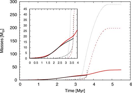
Mass of the core (solid line) and mass of the envelope (dashed line) as a function of the time for the in situ formation of a planet at 5 au. The black lines correspond to the giant planet formation model developed by Guilera et al. (2010, 2014), while the red lines correspond to PLANETALP. The grey line corresponds to a model using the gas accretion prescription given by Miguel et al. (2011). This simulation has been developed for a disc with a mass of 0.1 M_⊙, using γ = 1, R_c = 25 au, α = 10⁻⁴ and planetesimals of 10 km. The small square in the figure represents a zoom of the moment at which the gas accretion is triggered.

Open in new tab Download slide

It is important to note that the gas accretion rate on to planets is not considered as a sink term in the time evolution of the gas surface density profile. Therefore, our model controls that the mass of gas accreted by the planets of the system is not greater than 90 per cent of the mass of gas available in the disc at each time-step.

2.2.3 Fusion of embryos and planets with atmospheres

As we have already mentioned, embryos grow by accretion of gas and planetesimals, but they also grow due to collisions with each other. In this study, we consider that when the distance between two embryos becomes smaller than 3.5 mutual Hill radii, they merge into one object. From this, it is important to specify the mass of the resulting object, which will depend on the physical properties of the interacting bodies. In fact, if the embryos that participate in a collision are not very massive, their individual gaseous envelopes are negligible. In this case, we assume perfectly inelastic collisions, from which the mass of the resulting embryo will be the sum of the individual masses of the interacting embryos. If one or both of the interacting bodies is sufficiently massive to have a significant gaseous envelope, it is necessary to specify the core and envelope masses of the resulting body. On the one hand, the individual cores are perfectly merged in order to define the final core. On the other hand, the evolution of the gaseous envelopes is computed from the studies developed by Inamdar & Schlichting (2015). These authors analysed the formation of super-Earths and mini-Neptunes and examined how much gaseous envelope could have been accreted by planetary embryos before giant impacts and how much could be retained throughout the giant impact phase. Inamdar & Schlichting (2015) computed the global atmospheric mass-loss fraction χ_loss for ratios of envelope mass to core mass M_E/M_C between 10⁻¹ and 10⁻⁶ as a function of v_impm_imp/(v_escM_C), being v_impm_imp the impactor momentum, and v_esc the escape velocity of the target core of mass M_C. The values of χ_loss used in this work are those exposed in fig. 5 of Inamdar & Schlichting (2015). From these considerations, if bodies i and j collide, the core mass M_C of the resulting object will be given by

\begin{eqnarray} M_{{\rm C}} = M^{i}_{{\rm C}} + M^{j}_{{\rm C}}, \end{eqnarray}

(31)

where |$M^{i}_{{\rm C}}$| and |$M^{j}_{{\rm C}}$| are the core mass of the body i and j, respectively, while the final envelope mass M_E will be

\begin{eqnarray} M_{{\rm E}} = M^{i}_{{\rm E}}(1 - \chi _{{\rm loss}}^{i}) + M^{j}_{{\rm E}}(1 - \chi _{{\rm loss}}^{j}), \end{eqnarray}

(32)

where |$M^{i}_{{\rm E}}$| and |$M^{j}_{{\rm E}}$| are the envelope mass of the body i and j, respectively, and |$\chi _{{\rm loss}}^{i}$| and |$\chi _{{\rm loss}}^{j}$| the atmospheric mass loss fraction of the body i and j, respectively.

Finally, by conservation of angular momentum, we compute the semimajor axis of the resulting body by

\begin{eqnarray} a = \left(\frac{a^{0.5}_{i} \left(M^{i}_{{\rm C}} + M^{i}_{{\rm E}}\right) + a^{0.5}_{j}\left(M^{j}_{{\rm C}} + M^{j}_{{\rm E}}\right)}{M_{{\rm C}} + M_{{\rm E}}}\right)^{2}, \end{eqnarray}

(33)

being a_i and a_j the semimajor axis of the body i and j, respectively.

It is important to remark that the studies of Inamdar & Schlichting (2015) concerning the loss of atmospheric mass were developed for planets with masses in the range of the Neptunes and the so-called super-Earths and initial envelopes less than 10 per cent of the core mass. Due to the absence of works about atmospheric mass-loss by giant impacts in large atmospheres, we also used the results derived by Inamdar & Schlichting (2015) to treat collisions that involve giant planets. However, it is important to note that, in our study, the final mass of a giant planet is not sensitive to this consideration. This is due to the fact that a planet that is the final result of a merger between two previous planets is still growing in the disc. Thus, if this final planet has a significant core mass, it quickly accretes large amounts of gas. In fact, Broeg & Benz (2012) studied in detail the effect of this situation on the gas accretion rate of a planet. They found that initially, most of the envelope can be ejected, but afterwards, the gas is re-accreted very fast.

2.2.4 Type I and type II migration

A planet immersed in a protoplanetary disc modifies the local gas surface density and the mutual gravitational interactions between them, which lead to an exchange of angular momentum between the gas and the planet. This produces torques that cause that the planet migrates towards or away from the central star. Different types of migration regimes have been studied by many authors during the last two decades (Ward 1997; Tanaka, Takeuchi & Ward 2002; Masset, D'Angelo & Kley 2006; Paardekooper et al. 2010; Paardekooper, Baruteau & Kley 2011). These regimes modify the local density profile and the planets orbits in different ways depending on the mass of the planet and on the local properties of the disc.

Type I migration (Ward 1997) affects those planets that are not massive enough to open a gap in the gaseous disc. In idealized vertically isothermal discs, type I migration produces always inwards migration and very fast migration rates (Tanaka et al. 2002). Since type I migration is much faster than the gas dissipation time-scales of the discs and therefore much faster than the formation time-scales of the cores of giant planets, the survival of the planets, particularly of giant planets, results to be a difficult process to fulfill (Papaloizou et al. 2007). Although these migration rates have been corroborated by numerical simulations (D'Angelo, Kley & Henning 2003; D'Angelo & Lubow 2008), many authors had to reduce the migration rates by a constant factor in order to reproduce observations (Ida & Lin 2004a; Alibert et al. 2005; Mordasini et al. 2009; Miguel et al. 2011).

It is important to note that more recent works that consider non-isothermal discs (Paardekooper et al. 2010, 2011) have shown that type I migration could be outwards. Even in isothermal discs, type I migration could produce outwards migration if a full magnetohydrodynamic disc turbulence is considered (Guilet, Baruteau & Papaloizou 2013). Moreover, Benítez-Llambay et al. (2015) showed that the heating torques produced by a planet, while the process of solid accretion is given, are capable of slowing, halting or even reversing the migration of the planet in the protoplanetary disc if the mass of the planet is lower than 5M_⊕.

In order to be consistent with our model of planet formation, PLANETALP, we use the migration rates for isothermal discs of Tanaka et al. (2002) but considering different reduction factors f_migI, given by

\begin{eqnarray} \left(\frac{{\rm d}a_{{\rm P}}}{{\rm d}t}\right)_{{\rm migI}} = -2f_{{\rm migI}}a_{{\rm P}}\frac{\Gamma }{L_{{\rm P}}}, \end{eqnarray}

(34)

where |$L_{{\rm P}}=M_{{\rm P}}\sqrt{GM_{\star }a_{{\rm P}}}$| is the angular momentum of the planet, and the total torque is

\begin{eqnarray} \Gamma = \left(1.364 + 0.541\frac{{\rm dlog}\Sigma _{{\rm g}}}{{\rm dlog}a_{{\rm P}}}\right)\left(\frac{M_{{\rm P}}}{M_{\star }}\frac{a_{{\rm P}}\Omega _{{\rm k,P}}}{c_{{\rm s,P}}}\right)^{2}\Sigma _{{\rm g}}(a_{{\rm P}})a^{4}_{{\rm P}}\Omega ^{2}_{{\rm k,P}}.\nonumber \\ \end{eqnarray}

(35)

Remember that the sub-index P represents the location of the planet.

When a planet is massive enough to open a clear gap in the gas surface density profile, it undergoes type II migration. Crida, Morbidelli & Masset (2006) showed that a planet of mass M_P is able to clean more than 90 per cent of the gas around its orbit if

\begin{eqnarray} \frac{3}{4}\frac{H_{{\rm g}}}{R_{{\rm H}}} + \frac{50\nu }{a^{2}_{{\rm P}}\Omega _{{\rm k,P}}}\left(\frac{M_{\star }}{M_{{\rm P}}}\right) \le 1. \end{eqnarray}

(36)

Once the gap is opened, the orbital evolution of the planet is completely tied to the viscous evolution of the gas disc and, as long as the local mass of the disc is greater than the mass of the planet (‘disc-dominated type II migration’ following Armitage 2007), the planet migrates inwards at a rate given by

\begin{eqnarray} \left(\frac{{\rm d}a_{{\rm P}}}{{\rm d}t}\right)_{{\rm DD-migII}} = -\frac{3\nu }{2a_{{\rm P}}}, \end{eqnarray}

(37)

which is the same rate at which the gas moves in the disc (Ida & Lin 2004a). When the mass of the planet is high enough to be comparable to the local mass of the disc (‘planet-dominated type II migration’ following Armitage 2007), the migration rate is even lower and, as in Edgar (2007) and Mordasini et al. (2009), we calculate this migration rate as

\begin{eqnarray} \left(\frac{{\rm d}a_{{\rm P}}}{{\rm d}t}\right)_{{\rm PD-migII}} = -\frac{3\nu }{a_{{\rm P}}}\frac{\Sigma _{{\rm g}}(a_{{\rm P}})a^{2}_{{\rm P}}}{M_{{\rm P}}}. \end{eqnarray}

(38)

In this case, the migration rate depends not only on the viscosity of the disc but also on the gas surface density and on the mass of the planet.

2.3 Water distribution on embryos and planetesimals

We also incorporate a water radial distribution for the embryos and planetesimals in our model of planet formation. In order to be consistent with the initial surface density of planetesimals adopted previously (equations 2 and 3), the initial fraction per unit mass of water in embryos and planetesimals is given by

\begin{eqnarray} f_{{\rm H}_2{\rm O}}(R)= \left\lbrace \begin{array}{@{}l@{\quad }l@{}}0,& {\rm if}\ R \le R_{{\rm ice}}, \\ \\ \frac{\beta - 1}{\beta },& {\rm if}\ R > R_{{\rm ice}}. \end{array}\right. \end{eqnarray}

(39)

The time evolution of the water radial distribution of the planetesimals is calculated as the equation (9) is solved. Moreover, the amount of water in the embryos is calculated self-consistently as they accrete planetesimals, and when two embryos merge between them we consider that the amount of water of the new embryo is the sum of the amounts of water of the previous ones. We remark that we do not consider loss of water either by the accretion of planetesimals or the merger between embryos. Thus, the final amounts of water represent upper limits.

3 INITIAL CONDITIONS FOR OUR PLANETARY SYSTEMS

The main goal of this work is to find favourable scenarios and disc properties for planetary systems similar to our own with PLANETALP, to obtain initial conditions for the post-oligarchic growth of these systems ( Ronco & de Elía in preparation, from now on, PII). To do so, PLANETALP has been automated to develop several thousand planetary systems and to make a statistical study of population synthesis. Fig. 2 shows an schematic view of the operation of PLANETALP. In this section, we describe the initial conditions adopted to run PLANETALP taking into account that we are not interested in reproducing the actual exoplanet population, but we are interested in generating a great diversity of planetary systems without following any observable distribution in the disc parameters.

Figure 2.

Schematic view of the operation of PLANETALP.

Open in new tab Download slide

3.1 Scenarios and free parameters

As we have already mentioned, type I migration for idealized isothermal discs can be very fast, and thus, the time-scales of migration are usually shorter than the disc lifetime. As in Ida & Lin (2004a) and Miguel et al. (2011), we then consider different scenarios for the type I migration introducing the reduction factor f_migI, which considers possible mechanisms that can slow down the planet migration 10 and 100 times (f_migI = 0.1 and f_migI = 0.01). We also consider the extreme cases in where type I migration is not slowed down at all (f_migI = 1), and where it is not considered (f_migI = 0). It is important to remark that we are not considering dynamical torques in our model (Paardekooper 2014). These torques could slowed down significantly the migration rates estimated from the statical torques given by Tanaka et al. (2002). Sasaki & Ebisuzaki (2017) found that the M-a diagram calculated from a simple planet population synthesis model, based in the work of Ida & Lin (2004a) including statical and dynamical torques, can reproduce the observational exoplanet distribution around sun-like stars. It is important to note that this M-a diagram is similar to the M-a diagram obtained using statical torques and reduction factors in the type I migration rates.

Another important parameter for our model of planet formation is the size of the planetesimals. In the standard model of core accretion, both terrestrial planets and solid cores of gas giants are formed through the accretion of planetesimals (Safronov & Zvjagina 1969; Wetherill 1980; Hayashi 1981). However, the mechanisms for the formation of planetesimals and their initial sizes are still under debate (Johansen et al. 2014; Testi et al. 2014; Birnstiel, Fang & Johansen 2016). While collisional growth models could lead to the formation of sub-kilometre/kilometre planetesimals (Okuzumi et al. 2012; Dŗżkowska, Windmark & Dullemond 2013; Garaud et al. 2013; Kataoka et al. 2013; Arakawa & Nakamoto 2016; Kobayashi, Tanaka & Okuzumi 2016), gravitational collapse models predict the formation of tens/hundreds kilometre planetesimals (Johansen et al. 2007; Cuzzi, Hogan & Shariff 2008; Johansen, Youdin & Lithwick 2012; Simon et al. 2016; Schäfer, Yang & Johansen 2017). Moreover, the size distribution of the asteroid belt can be reproduced by collisional evolution models, using both an initial population of big planetesimals (Morbidelli et al. 2009) and an initial population of small planetesimals (Weidenschilling 2011).

In this work, as in Fortier et al. (2013), we consider scenarios with different sizes for the planetesimals (r_p = 100 m, 1 km, 10 km and 100 km), but we consider a single size per simulation. It is important to note that, while big planetesimals (r_p ≳ 10 km) are mainly governed by the quadratic regime for the determination of the radial drift and solid accretion rates, small planetesimals (r_p ≲ 1 km) can be in different drag regimes along the disc.

We consider random values from uniform distributions for all the free parameters because we are interested in developing a great diversity of planetary systems without following any observable parameter distribution. However, we take into account that the bounds of the parameter ranges are obtained from previous works. Following Andrews et al. (2009, 2010), we consider the mass of the disc, M_d, between 0.01 M_⊙ and 0.15 M_⊙, the characteristic radius R_c between 20 au and 50 au, and the density profile gradient γ between 0.5 and 1.5. The factor β is taken randomly between 1.1 and 3 given that, in our Solar system, Lodders (2003) usually takes a value of approximately 2 and Hayashi (1981) adopts a value of 4. It is important to note that a value of β = 1.1 represents an amount of 9 per cent of water by mass, while a value of β = 3 represents an amount of 66 per cent of water by mass on embryos and planetesimals at the beginning of the simulations and beyond the snowline, following equation (39). The viscosity parameter α for the disc and the rate of EUV ionizing photons f₄₁ have a uniform distribution in log between 10⁻⁴ and 10⁻², and between 10⁻¹ and 10⁴, respectively (D'Angelo & Marzari 2012).

Since the maximum value of the mass of the discs considered is relatively high and since this can lead to the occurrence of gravitational instabilities, our model checks, according to the Toomre criterion (Toomre 1964), given by

\begin{eqnarray} Q = \frac{c_{{\rm s}}\Omega _{{\rm k}}}{\pi G \Sigma _{{\rm g}}}, \end{eqnarray}

(40)

the stability of our discs. When Q > 1, discs are considered unstable. It is important to remark that all the considered discs in our simulations result to be stable throughout their entire extent.

Other parameters are kept constant for all the simulations. As we are particularly interested in the formation of Solar system analogues, the mass of the central star is always 1 M_⊙ and the metallicity is [Fe/H] = 0. Also, the planetesimal and embryo densities are considered constant and to be 1.5 and 3 g cm⁻³, respectively.

Regarding the embryo population, we consider an embryo distribution between 0.1 and 30 au. These embryos are separated by 10 mutual Hill radii, assuming circular and coplanar orbits, and their initial masses, which are of the order of the mass of the Moon, are given by the transition mass between the runaway and the oligarchic regime (Ida & Makino 1993) as

\begin{eqnarray} M_{{\rm oli}} = 1.6R^{6/5}10^{3/5}m^{3/5}_{{\rm p}}\Sigma ^{3/5}_{{\rm p}}M^{-1/5}_\star \end{eqnarray}

(41)

where m_p is the mass of the planetesimals.

Finally, with the aim of finding the most suitable scenarios and parameters that provide us with Solar system analogues we perform 1000 simulations per each combination between f_migI and r_p. This is, we form 16 000 different planetary systems that evolve in time until the gas of the disc dissipates. From now on, when we talk about formation scenarios, we are referring to all the combinations between f_migI and r_p.

3.2 The disc dissipation time-scale

Another important parameter that determines the final configuration of a planetary system during the gaseous phase is the gas-disc dissipation time-scale, τ. Haisch, Lada & Lada (2001) and Mamajek (2009) have observed young stars in clusters of different ages and they suggested that protoplanetary discs have characteristic lifetimes between 3 and 10 Myr. More recently, Pfalzner, Steinhausen & Menten (2014) showed that, taking into account that the previous works present observational biases, gas discs could last much longer than 10 Myr.

In our model, unlike Miguel et al. (2011) for example, wherein the evolution of the gas is represented by an exponential decay law, the gas disc evolves due to the viscous accretion and photoevaporation processes. Both phenomena together determine the lifetime of the gas, τ. Therefore, we need to form planetary systems whose combinations between the viscosity parameter α, the EUV rate f₄₁, the mass of the disc M_d, the characteristic radius of the disc R_c, and the surface density gradient γ make the gas discs of these systems to dissipate on time-scales according to the results of the previous mentioned works. To do this, we run a version of PLANETALP that is limited to the study of the evolution in time of the gas disc. This is, we ‘turn off’ the evolution of the planetesimal surface density and the evolution of the embryo population. We then generate, using a von Neumann acceptance–rejection method, as many gas discs with dissipation time-scales between 1 and 12 Myr as we need; this is, 16 000 combinations of all the parameters to develop complete planetary systems.

Fig. 3 shows the time-scale (in Myr) versus mass of the disc (in solar masses) plane. Each point represents a set of parameters randomly taken. The 16 000 red points represent sets whose combinations between all the parameters obtained a disc of gas that dissipated between 1 and 12 Myr. We find a mean value of τ of 6.45 Myr with a dispersion of σ = 2.67 Myr. The black points are those sets that resulted in discs dissipating in less than 1 Myr or in more than 12 Myr. These last sets are then discarded for our simulations.

Figure 3.

Dissipation time-scale in Myr as a function of the mass of the disc in solar masses for all the simulations performed. Each point represents a set of parameters randomly taken that is going to build a final planetary system. The red points represent those sets whose combinations between all the parameters managed to obtain a dissipation time-scale τ between 1 and 12 Myr. The black points are those sets that did not managed to obtain a suitable τ and are not going to be taken into account.

Open in new tab Download slide

4 RESULTS

The main goal of this work is to find, through the population synthesis analysis developed with our model of planet formation, sets of appropriate initial conditions to study, in a future work (PII), the post-oligarchic evolution of planetary systems similar to our own with N-body simulations. However, through the development of the 16 000 simulations, which were performed randomly and uniformly varying the parameters of the disc, we found a great diversity of planetary systems architectures, not only Solar system analogues.

4.1 General results

To classify the diversity of planetary systems, we define general properties for the different types of planets. On the one hand, gas giant planets present an envelope that is greater than the mass of the core. Within this category, we can find Jupiter-like or Saturn-like planets. The difference between them is that we consider that Jupiter-like planets manage to open a gap in the disc or their total mass is greater than 200M_⊕. On the other hand, icy giant planets present envelopes greater than 1 per cent of the core mass but must have envelopes smaller than the core mass. At last, rocky planets present envelopes smaller than 1 per cent of their core mass. Having classified the final planets, from all the diversity of planetary systems developed, we can distinguish three global kinds of planetary systems that we classify as follows:

Rocky planetary systems: Planetary systems which are formed only by rocky planets, without gas or icy giants.
Icy giant planetary systems: These planetary systems can harbour rocky planets but they must present at least one icy giant planet analogue to a Neptune-like planet, or a hot/warm Neptune-like planet.
Gas giants planetary systems: Planetary systems that must harbour at least one giant planet (in this global characterization we do not distinguish the location of the giant), but can also contain rocky and icy giant planets.

In this work, we are particularly interested in those planetary systems which, at the end of the gas phase, present similarities to our own Solar system, and so we classify them as follows:

Solar system analogues (SSAs): Planetary systems that host only rocky planets in the inner zone of the disc and at least one giant planet beyond 1.5 au.

SSAs represent a subkind of those planetary systems with gas giants. Table 1 shows the general percentages of each kind, including the percentage that SSAs represent respect to the total of the performed simulations. Although the scope of this work is to focus only on SSA, we will mention some general results of the developed simulations that are in good agreement with previous works.

Table 1.

Open in new tab

Final percentages of planetary systems with respect to the total of the developed simulations.

Planetary system	Final percentage
Rocky planetary systems	64.46%
Icy giant planetary systems	13.4%
Gas giant planetary systems	22.14%
Solar system analogues	4.3%

Table 1.

Open in new tab

Final percentages of planetary systems with respect to the total of the developed simulations.

Planetary system	Final percentage
Rocky planetary systems	64.46%
Icy giant planetary systems	13.4%
Gas giant planetary systems	22.14%
Solar system analogues	4.3%

Following Table 1, it is clear that rocky planetary systems represent the vast majority, indeed, more than 60 per cent of the total of the simulated planetary systems. Moreover, we can find this kind of systems in all the formation scenarios considered. In fact, rocky planetary systems represent more than 40 per cent of the planetary systems in each formation scenario for all of them but one, wherein represent ∼20 per cent. Finally, we can also find them in the whole range of disc masses considered, between 0.01 M_⊙ and 0.15 M_⊙. This result is in good agreement with the results obtained by Miguel et al. (2011), although they followed observable distributions for the most important disc parameters and although they only considered planetesimals of 10 km.

Fig. 4 shows maps of density of the different planetary systems for each formation scenario. Rocky planetary systems are significantly more favourable in formation scenarios with big planetesimals and low-moderate/null type I migration rates, although, as we mentioned before, we find them in each of all the formation scenarios. This is a natural consequence of the fact that planetesimal accretion rates are smaller for big planetesimals, and thus, the formation of massive cores generally requires formation time-scales that exceed the characteristic dissipation time-scales of the discs. Besides, the smaller the type I migration rate, the smaller the probability of merger between embryos, and thus, the formation of massive cores by this mechanism. It is also important to note that a significant number of rocky planetary systems is formed by small planetesimals and low-moderate/null type I migration rates. This is due to the fact that Fig. 4 does not represent explicitly the dependence with the mass of the discs. As we adopted that the mass of the disc is uniformly distributed between 0.01 M_⊙ and 0.15 M_⊙, there is a significant percentage of systems in which the total mass of the disc is not enough to form massive cores, and consequently, icy giant or gas giant planets.

Figure 4.

Maps of density of rocky planetary systems (left), icy giant planetary systems (middle) and gas giant planetary systems (right). The grey-scale represents the number of planetary systems in each formation scenario. For each scenario, the sum of rocky, icy giant and gas giant planetary systems is equal to 1000.

Open in new tab Download slide

The opposite case is given by the icy giant planetary systems. These planetary systems are mainly formed in scenarios with small planetesimals and large type I migration rates. The planetesimal accretion rates are greater for smaller planetesimals, situation that lead to the quickly formation of several Earth-cores beyond the snowline. However, large type I migration rates produces that these cores quickly reach the inner edge of the disc, avoiding the formation of gas giants. Therefore, on the one hand, high type I migration rates could lead to the merge of embryos, and thus, the formation of massive cores as we mentioned before. But, on the other hand, high type I migration rates also cause the planets to quickly get into the inner zone, and fail in the gas giant formation.

Finally, gas giant planetary systems are majority for small planetesimals and low-moderate/null type I migration rates. As it was already mentioned, small planetesimals favour the formation of massive cores, and low-moderate/null type I migration rates avoid the planet to drop into the inner edge of the disc, allowing the planet to trigger the gaseous runaway growth. However, it is important to note that we find gas giants in scenarios with high type I migration rates. About a 70 per cent of the planetary systems formed in scenarios with high type I migration rates, considering all the chosen planetesimal sizes, present Hot/Warm-Jupiters within 0.5 au. However, taking into account all the formation scenarios that form giant planets, not only those with high type I migration rates, the planetary systems with Hot/Warm-Jupiters represent the 43 per cent of Gas Giant planetary systems. Moreover, those planetary systems with Hot/Warm-Jupiters represent only a 9.5 per cent of the total of the developed simulations. Thus, although we find higher percentages of Hot-Jupiter occurrences than those predicted observationally, which are ∼1 per cent (Marcy et al. 2005; Cumming et al. 2008; Mayor et al. 2011; Wright et al. 2012), Wang et al. (2015) concluded that the current knowledge of stellar properties and the stellar multiplicity rate is yet very limited to reach quantitative results for the Hot-Jupiter occurrence.

We remark again, that these density maps do not take into account the dependency with the properties of the disc, i.e. the mass of the discs, the exponent γ, the characteristic radius and the factor β.

4.2 Solar system analogues

Of the performed simulations, we found that only 688 protoplanetary discs formed SSAs, this represents only a 4.3 per cent of the total. Table 2 shows the percentages of SSAs for each formation scenario and Fig. 5 shows γ versus M_d planes for each formation scenario. In this figure, each point represents a formed planetary system with a particular set of disc parameters. The coloured points represent SSA, the grey points are the rest of the planetary systems performed in which we are not going to focus in this work. The colour-scale shows the dissipation time-scale of the gas disc for each planetary system. As we can see in Table 2 and Fig. 5 , we do not find SSAs in scenarios with non-reduced type I migration. This is due to the fact that, as we have already mentioned, type I migration without any reduction factor causes that giant-forming planets in the outermost zone of the disc migrate to within 1.5 au in time-scales smaller than the dissipation of the gas disc, regardless of the size of the planetesimals considered. Clearly, formation scenarios of low (or none) type I migration rates and small planetesimals (100 m and 1 km) are the most favourable for the formation of SSAs. Since the planetesimal accretion rates are higher for small planetesimals, the rapid formation of massive cores before the dissipation of the gas is favoured. Otherwise, for large planetesimals, the formation time-scales of massive nuclei are not high enough to trigger the growth of the gaseous envelope and to form giant planets in time-scales according to the disc lifetime.

Figure 5.

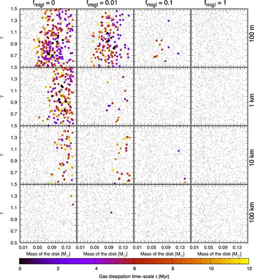
Distribution of the planetary systems produced by PLANETALP in a plane M_d–γ. SSAs are represented with coloured points. The colour-scale represents the dissipation time-scale of each disc. Grey points represent the rest of the planetary systems that are not SSAs. Black diamonds are those SSAs with all their disc parameters between ±σ. Each row and each column shows the results for the different formation scenarios.

Open in new tab Download slide

Table 2.

Open in new tab

Percentage of SSAs found in each formation scenario.

Planetesimal size	f_migI = 0	f_migI = 0.01	f_migI = 0.1	f_migI = 1
100 m	26.90%	14.90%	1.10%	0%
1 km	16.40%	1.4%	0%	0%
10 km	5.10%	2.40%	0.3%	0%
100 km	0.2%	0.1%	0%	0%

Planetesimal size	f_migI = 0	f_migI = 0.01	f_migI = 0.1	f_migI = 1
100 m	26.90%	14.90%	1.10%	0%
1 km	16.40%	1.4%	0%	0%
10 km	5.10%	2.40%	0.3%	0%
100 km	0.2%	0.1%	0%	0%

Table 2.

Open in new tab

Percentage of SSAs found in each formation scenario.

Planetesimal size	f_migI = 0	f_migI = 0.01	f_migI = 0.1	f_migI = 1
100 m	26.90%	14.90%	1.10%	0%
1 km	16.40%	1.4%	0%	0%
10 km	5.10%	2.40%	0.3%	0%
100 km	0.2%	0.1%	0%	0%

Planetesimal size	f_migI = 0	f_migI = 0.01	f_migI = 0.1	f_migI = 1
100 m	26.90%	14.90%	1.10%	0%
1 km	16.40%	1.4%	0%	0%
10 km	5.10%	2.40%	0.3%	0%
100 km	0.2%	0.1%	0%	0%

4.2.1 Solar system analogue architectures

As we already mentioned, SSAs must harbour at least one giant planet beyond 1.5 au and rocky planets in the inner regions of the disc. However, the architectures of the SSAs found are quite different, and not all of them present icy giants or only one gas giant planet. Taking into account all the SSAs, without distinguishing between planetesimal sizes or migration rates, the most representative architectures found amongst the SSAs are those that present between 1 and 3 gas giants, between 0 and 4 icy giants and between 100 and 200 rocky planets along the disc. In fact, the mean of the number of gas giants is 2, with a dispersion of ∼1, the mean of the number of icy giants is also 2, with a dispersion of ∼2, and the mean of the number of rocky planets is 150, with a dispersion of ∼47. Particularly, Fig. 6 displays histograms showing the percentage of SSAs that present one, two, three, four or five gas giants, and also shows how many systems present different numbers of icy giants and rocky planets, but differentiating the systems according to the size of planetesimals and migration rates. For planetesimals of 100 km, only one giant planet is formed in the only three systems found for low or null type I migration. These systems also harbour only one, or none, icy giant, but a significant number of rocky embryos, some of them in the outer part of the disc. For these big planetesimals, we do not find SSAs formed with moderate and non-reduced type I migration rates. The formation of two giant planets is more likely for low or null type I migrations rates and scenarios with planetesimals of 10 km, while the formation of only one gas giant is more favourable for moderate type I migration rates. It is important to note that, in both cases, there is a not negligible probability to form systems with three or four giant planets. These systems also harbour preferentially a small number of icy giants. However, we found that for the case of null or low type I migration rates, it is possible to find SSAs that harbour until 8 icy giants. These kind of systems also present preferably between 100 and 200 rocky embryos. For small planetesimals of 1 km and 100 m, we find similar results. In both cases, planetary systems preferentially harbour one or two giant planets, with the difference that no giant planet is formed for planetesimals of 1 km of radius for moderate type I migration rates. In both cases, a small number of icy giants is also expected. Finally, a large number of rocky planets are expected in such systems when the gas of the disc is dissipated. It is important to remark that the stability and dynamical evolution of these kind of systems after the gas dissipation will be discussed in the forthcoming paper.

Figure 6.

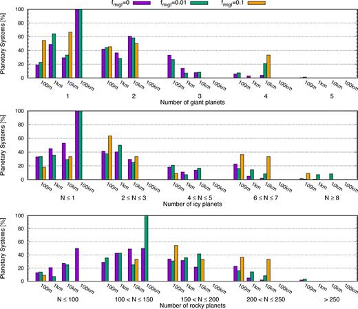
Histograms showing how many gas giants, icy giants and rocky planets present in each SSA formation scenario.

Open in new tab Download slide

4.2.2 Favourable disc parameters

Taking into account all the SSAs, Table 3 shows the ranges, mean and dispersion values for the disc parameters. As we can see, we can find SSAs for all the ranges considered of γ, R_c, α and τ. However, we do not find SSAs for low-mass discs (M_d < 0.04 M_⊙) because low-mass discs have not enough solid material to form massive cores before the disc dissipation time-scales. Similar results were found by Thommes et al. (2008) and Miguel et al. (2011). Although we find SSAs for almost all the values in the ranges of the free disc parameters, they are preferentially formed for massive disc (<M_d > =0.1 M_⊙), smooth surface densities profiles (<γ > =0.95), moderate values for the disc characteristic radius (<R_c > ∼33 au), small values of the α-viscosity parameter (<α > =3.4 × 10⁻⁴), and moderate time-scales for the disc dissipation (<τ > ∼6.5 Myr). It is worth mentioning that only 20 SSAs have all their disc parameters between the dispersion values, ±σ. These planetary systems are represented with black diamonds in Fig. 5. This represents only a ∼3 per cent of the total SSAs. All these systems are formed considering small planetesimals (100 m and 1 km) and adopting null or low type I migration rates.

Table 3.

Open in new tab

Ranges, means and dispersion values of the disc parameters that formed SSAs.

Disc	Range	Mean	σ
parameter
M_d	0.04–1.15 M_⊙	0.10 M_⊙	0.027 M_⊙
γ	0.5–1.5	0.95	0.27
R_c	20–50 au	32.8 au	8.73 au
α	10⁻⁴–10⁻²	3.4 × 10⁻³	2.8 × 10⁻³
τ	1.65–11.96 Myr	6.45 Myr	2.67 Myr

Disc	Range	Mean	σ
parameter
M_d	0.04–1.15 M_⊙	0.10 M_⊙	0.027 M_⊙
γ	0.5–1.5	0.95	0.27
R_c	20–50 au	32.8 au	8.73 au
α	10⁻⁴–10⁻²	3.4 × 10⁻³	2.8 × 10⁻³
τ	1.65–11.96 Myr	6.45 Myr	2.67 Myr

Table 3.

Open in new tab

Ranges, means and dispersion values of the disc parameters that formed SSAs.

Disc	Range	Mean	σ
parameter
M_d	0.04–1.15 M_⊙	0.10 M_⊙	0.027 M_⊙
γ	0.5–1.5	0.95	0.27
R_c	20–50 au	32.8 au	8.73 au
α	10⁻⁴–10⁻²	3.4 × 10⁻³	2.8 × 10⁻³
τ	1.65–11.96 Myr	6.45 Myr	2.67 Myr

Disc	Range	Mean	σ
parameter
M_d	0.04–1.15 M_⊙	0.10 M_⊙	0.027 M_⊙
γ	0.5–1.5	0.95	0.27
R_c	20–50 au	32.8 au	8.73 au
α	10⁻⁴–10⁻²	3.4 × 10⁻³	2.8 × 10⁻³
τ	1.65–11.96 Myr	6.45 Myr	2.67 Myr

4.2.3 Evolution and final configuration of Solar system analogues

In this section, we describe the general characteristics of the evolution in time of a SSA, and also show the final configurations of the most representative SSAs of each formation scenario, which are composed of the following:

An embryo distribution that provide us with information about the semimajor axis, mass of the core, mass of the envelope, mass of water due to the accretion of planetesimals and mass of water due to the fusion with other embryos of each final body.
A planetesimal surface density, eccentricity and inclination profiles.

These final configurations are going to serve as initial conditions to analyse the post-oligarchic stage of planet formation, via N-body simulations (PII).

Fig. 7 shows the evolution in time, represented by the colour-scale, of a representative SSA for the formation scenario without type I migration and with planetesimals of 1 km. The parameters of this particular system are M_d = 0.13 M_⊙, γ = 0.92, R_c = 34 au, α = 1.1 × 10⁻³, and a dissipation time-scale of τ = 6.65 Myr. The factor that represents the amount of solid material condensed beyond the snowline, at 2.7 au, is β = 1.96, in this example. Fig. 7(a) represents the time evolution of the embryo distribution. The small red points linked by lines represent the initial embryo distribution. These embryos start to grow due to the accretion of planetesimals within their feeding zones. In time, as they grow, if the distance between them is less than 3.5 Hill radius they merge into one object. When the cores reach a critical mass, which is approximately 10M_⊕, they start to accrete significant amounts of gas until they achieve their final masses and the disc is dissipated. Figs 7(b) and (c) represent the evolution in time of the gaseous component of the disc. The gas surface density profile (b), which is plotted every 0.1 Myr, begins to decrease and to expand in the radial direction due to the disc angular momentum conservation. At approximately 2 Myr, a gap is opened in the disc due to the photoevaporation process. As a consequence, the gas in the inner zone of the disc, inside the gap, rapidly falls to the central star, while the gas in the outer zone continues its evolution for a few million years. The mass of the gas in the disc decreases as it is shown in Fig. 7(c). The planetesimal surface density (Fig. 7d) evolves in time due to the radial drift and due to the embryos, which accrete and excite them, increasing their eccentricities (Fig. 7e) and inclinations (Fig. 7f). As time advances, the planetesimal profile decreases, and the inner zone of the disc quickly runs out of planetesimals. This is mainly due to the fact that the planetesimal accretion rates are higher in the inner zone where the planetesimal surface density is initially higher. This favours the formation of many, low-mass rocky planets very close to each other, which accrete all the available solid material. These embryos do not merge between them due to the fact that their feeding zones are very narrow, an thus, they do not grow enough to be separated less than 3.5 mutual Hill radius (specially, very close to the star). Besides, the formation of two giant planets (see Fig. 7a) helps to remove planetesimals between 10 and 15 au. At the end, when there is no more gas in the disc, there are only planetesimals behind 15 au. This remnant of planetesimals (represented with the blue line) present final eccentricity and inclination profiles according to the blue lines in Figs 7(e) and (f), respectively. It is important to note that these eccentricity and inclination profiles along the disc have physical sense only in the region where there is still presence of planetesimals, for this particular case, beyond ∼ 15 au.

Figure 7.

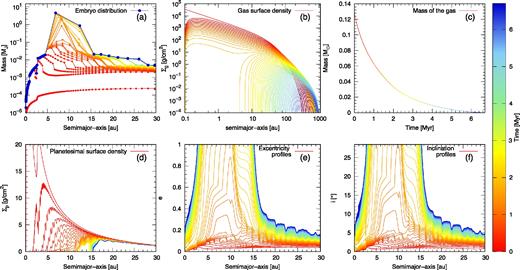
Example of the evolution in time of the embryo distribution (a), the gas surface density (b), the mass of the disc (c), the planetesimal surface density (d) and the eccentricity and inclination profiles (e and f, respectively) of an SSA with planetesimals of 1 km and without type I migration. The parameters of this disc are M_d = 0.13 M_⊙, γ = 0.92, R_c = 34 au, α = 1.1 × 10⁻³ and τ = 6.65 Myr. Finally, β = 1.96. The colour-scale represents the time evolution of the system, and each profile is plotted every 0.1 Myr.

Open in new tab Download slide

As we mentioned before, the aim of this work is to find suitable initial conditions for SSAs to develop N-body simulations; thus, Fig. 8 shows representative final configurations of SSAs in all the formation scenarios in which they were found. Each panel shows the final embryo distribution with the final planetesimal density profile of each system at the top, and the final planetesimal eccentricity and inclination profiles in the bottom. The colour-scale represents the percentage of water by mass.

Figure 8.

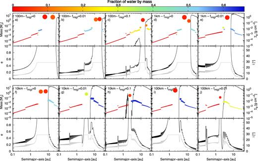
Representative planetary configurations at the end of the gaseous phase of all the formation scenarios that present SSAs in a mass versus semimajor axis versus planetesimal surface density plane, and eccentricity versus semimajor axis versus inclination profile plane. Each coloured point represents a final planet, the solid black line in all the planetary systems represents the final planetesimal density profile at that time. Under these planet distributions and planetesimal profiles, we can see the final planetesimal eccentricity and inclination profiles in black and grey lines, respectively. These final profiles are only important for those regions in the disc where there is still a planetesimal population. The colour-scale represents the final amounts of water by mass in each planet and the size of each planet is represented in logarithmic scale. The final planetary system obtained with planetesimals of 1 km and without type I migration (d) is the same planetary system exemplified on Fig. 7.

Open in new tab Download slide

Although all this planetary systems are SSAs, they present global differences regarding on the location of the giant planets and on the final planetesimal surface density profiles. On the one hand, as the size of the planetesimals and the reduction factor of type I migration increase, the location of the giant planets changes, moving inwards. On the other hand, also the planetesimal remnant until 30 au increases towards the central star. The final location of the giant planet depends on several phenomena. As it was shown by Guilera et al. (2011), the competition between the planetesimal accretion time-scales and the planetesimal migration time-scales regulates the formation of a giant planet. These authors found that these two time-scales depend on the planetesimal size and on the location of the planet with respect to the central star. Thus, the optimal location in the disc for the formation of a massive core, precursor of a giant planet, is different for different planetesimal sizes. Besides, the main properties of the protoplanetary disc, i.e. the slopes of the surface densities, the jump in the position of the snowline due to the condensation of volatile material and the characteristic radius, can play an important role in the formation of a giant. In fact, Guilera et al. (2011) found that for smooth slopes, the formation of a giant planet is optimized in the outer part of the disc for scenarios with small planetesimals (r_p < 100 m). Moreover, another important phenomenon that could change the optimal location of the formation of a giant planet is the merger between several planets.

As an example, Fig. 9 shows the time of cross-over as a function of the position of the planet in the disc. The time of cross-over is the time at when the mass of the envelope of a planet equals the mass of the core (mass of cross-over) and the gaseous runaway triggers. The black points and black diamonds in Fig. 9 represent the in situ formation of an isolated planet, located at different positions between 2 and 15 au, for the same disc parameters of the formation scenario of Figs 8(d) and (i), respectively. As we can see, for scenarios with planetesimals of 1 km, the optimal location for the formation of a giant planet is around 5 au, while for scenarios with planetesimals of 100 km, the optimal location is 3 au. It is worth mentioning that we find similar results between the scenarios of 1 km and 100 m, and between the scenarios of 10 and 100 km. However, when we include the formation of the whole complete system, the optimal location for the formation of the giant can change and can move away from the central star. As Fig. 9 displays for scenarios with planetesimals of 1 km, the red point in Fig. 9 shows the location at where the first planet of the system reached the mass of cross-over. This situation shows that, when the simultaneous formation is considered, the formation of giant planets can be optimized in outermost regions. This is due to the multiple mergers between embryos that have taken place during the formation of the system. For planetesimals of 100 km, the location of the giant planet is optimized a little bit away from the position found for the isolated formation. In this scenario, as the embryos do not grow enough to increase their Hill radius, the rate of mergers is lower.

Figure 9.

Cross-over time as a function of the initial position of a planet, for the isolated formation, and for scenarios with planetesimals of 1 and 100 km, and without type I migration. The black dots show the isolated formation in scenarios with planetesimals of 1 km. The disc parameters of this formation scenario are the same as in Fig. 8(d), which dissipates in 6.64 Myr. The black diamonds show the isolated formation in scenarios with planetesimals of 100 km, and the disc parameters of this formation scenario are the same as in Fig. 8(i), which dissipates in 7.12 Myr. The red dot and red diamond show the location and time when the first planet of each system (corresponding to Figs 8(d) and (i), respectively) reached the mass of cross-over.

Open in new tab Download slide

Continuing with the description of Fig. 8, if we only consider those planetary systems without type I migration, to distinguish the effect caused by the increase in the planetesimal size (see Figs 8a, d, f and i), we can see that for planetesimals of 100 m, the giant planets form in the outer regions of the disc. Since the accretion rates are higher than for big planetesimals, massive cores form in a shorter time-scale, and thus, the planets in the outer region can merge between them before the dissipation of the gas disc, giving rise to giant planets in the outer zones. These giants clean their surroundings of planetesimals, leaving a very small remnant almost beyond 20 au. Despite both planets are Jupiter-analogues, the innermost giant opened a gap in the disc and moved inwards through type II migration, while the outermost did not. A brief discussion about why a giant planet with ∼4.8M_J did not opened a gap in the disc is discussed in the next section.

Following with the scenario of planetesimals of 1 km (Fig. 8d), as the planetesimal accretion rates decrease with respect to the previous scenario, those planets in the outer zone grow achieving masses between ∼1.5M_⊕ and ∼6.5M_⊕. These planets do not grow enough to merge between them and thus, we do not find giants on the outer part of the disc. Moreover, they do not remove their feeding zones completely and do not empty them from planetesimals. Therefore, at the end of the gas phase, a population of planets of several Earth masses and a population of planetesimals coexist in the outermost regions of the disc. A similar situation occurs for scenarios with planetesimals of 10 km (Fig. 8f). But in this case, the optimal location for the formation of the giants moves inwards a little bit. At last, for scenarios with planetesimals of 100 km, the formation of giant planets is optimized near the snowline, at ∼3 au. In Fig. 8(i), the only formed giant reached 2 au due to the fact that opens a gap in the disc and moves through type II migration.

Regarding the population of planetesimals, a remnant of planetesimals survived at the end of the gaseous phase in the majority of the performed simulations inside 30 au. However, it is worth mentioning that we found a few simulations of planetary systems without planetesimals inside 30 au for scenarios with planetesimals of 100 m. How this result will affect, or not, the post-oligarchic growth of the planets in these system is an analysis that we are going to take into account in our next work.

Another important thing to note, with respect to the final planetesimal population, is that some planetary systems present a small remnant of planetesimals inside the location of the giant planet. This can be seen, for example, in Figs 8(c) and (h). Particularly, the remnant of planetesimals in the formation scenario of Fig. 8(h) is located between 2 and 3 au. This seems to be of interest, since it could lead to the formation of an asteroid belt between the terrestrial-planet forming region and the giant planets. However, it will be important to analyse in a future if these planetesimals would survive in the disc, since after the dissipation of the gas they present eccentricities and inclinations greater than ∼0.4 and 10°.

One of the differences between our model of planet formation and other population synthesis models is that we include a detailed treatment of the orbital evolution of the planetesimal population. This improvement allows us to obtain more realistic planetesimal surface density, eccentricity and inclination profiles at the end of the gaseous phase to use as initial conditions for the planetesimal population in the post-gas evolution of these systems.

4.2.4 Gap opening planets

In SSAs, the frequency of a gap opening planet in the disc is relatively low. For each forming-giant planet that opens a gap in the disc, there are 5.5 giant planets that did not. As we described in Section 2.2.4, the condition that a giant planet must fulfill to open a gap is that proposed by Crida et al. (2006). This condition depends basically on the mass and the location of the planet and on the viscosity and the height scale of the disc. More explicitly, this condition depends on the sum of two terms: the first term involves the ratio between the height scale of the disc and the Hill radius of the planet, this last is a function of the mass and position of the planet; the second term involves the ratio between the viscosity of the disc and a function of the location and mass of the planet. Thus, the opening of a gap is favoured by massive planets, and low viscosity and flat/thin discs (i.e. discs with small aspect ratios H_g/R). However, our model considers a flare disc, hence, H_g/R ∝ R and it increases with the distance to the central star. This situation coupled with having moderate/high values of the viscosity of the discs results in the low occurrence of gap opening for giant planets in our model. As an example, Fig. 10 shows the minimum mass needed to open a gap, adopting the criteria developed by Crida et al. (2006), as a function of the planet semimajor axis for discs with different viscosities. We show the limit cases for the values of the α parameter adopted in this work and the mean value (± the dispersion) of such parameter. We also plotted the curve corresponding to the planetary system described in Fig. 8(a) (grey line) and also the final location of both giant planets of that system. We can see that the inner Jupiter-analogue has a final mass greater than the minimum needed to open a gap in such disc. However, the outer Jupiter-analogue, despite of having a mass of ∼4.8M_J, did never achieved the minimum mass needed to open a gap.

Figure 10.

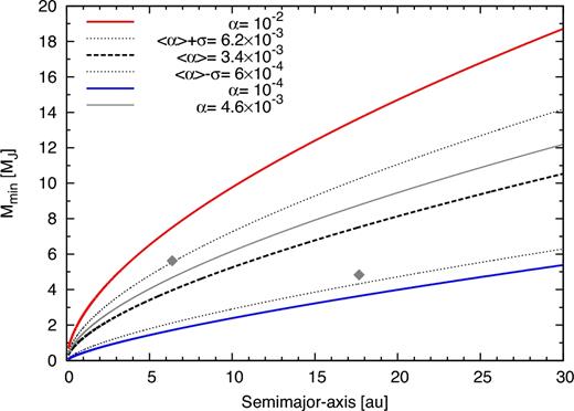
Minimum mass needed to open a gap as a function of the planet semimajor axis according to Crida et al. (2006). The red curve corresponds to a disc with α = 10⁻² (the upper-limit case), while the blue curve corresponds to a disc with α = 10⁻⁴ (the lower-limit case). The black dashed line represents a disc with mean value of α (for the SSAs), <α > =3.4 × 10⁻³, and the black dotted lines represent discs with <α > ±σ. Finally, the grey curve represents the system described in Fig. 8(a). The grey diamonds represent the final mass and final semimajor axis of the giant planets of this system.

Open in new tab Download slide

4.2.5 Water accretion on planets of the habitable zone

A point of interest for our SSA is to analyse the final amounts of water by mass in those planets that remain, at the end of the gaseous phase, in the habitable zone. Taking into account the classical definition, the habitable zone is defined as the range of heliocentric distances at which a planet can retain liquid water on its surface (Kasting, Whitmire & Reynolds 1993). Ten years later, Kopparapu et al. (2013a,b) proposed that our Solar system presents a conservative habitable zone determined by loss of water and by the maximum greenhouse effect provided by a CO₂ atmosphere between 0.99 and 1.67 au. Moreover, these authors proposed that there is also an optimistic habitable zone between 0.75 and 1.77 au, limits that were estimated based on the belief that Venus has not had liquid water on its surface for the last 1 billion years and that Mars was warm enough to maintain liquid water on its surface. Although the definition of the habitable zone is a topic under permanent debate, and although there is no guarantee that a planet inside this region will be potentially habitable, we consider this definition just as a first approximation. As it was mentioned before in Section 2.3, both embryos and planetesimals present, at the beginning of our simulations, a water radial distribution. As the embryos grow and the planetesimal surface density evolves, also the amount of water on each body changes. It is important to notice that, as we can see in Fig. 8 those planets in SSA that remain within the habitable zone at the end of the gaseous phase do not present any water contents. This is due to the fact that the embryo distribution beyond the snowline act as a barrier, preventing that water-rich planetesimals from the outer zone are accreted by embryos of the inner zone. In addition, the low and null type I migration rates also prevent that embryos from beyond 2.7 au reach the habitable zone. Although these planets are dry when the gas in the disc dissipates, this does not mean that they cannot acquire significant amounts of water for the possible development of life during the post-oligarchic growth stage via, for example, accretion of wet embryos or planetesimals from beyond the snowline. This analysis is out of the scope of this work but is going to be taken into account in PII.

5 SUMMARY AND DISCUSSION

During the last years, advances in observational astronomy have allowed us to increase the sample of confirmed exoplanets very quickly. This sample, which continues to grow day by day, has motivated the theoretical astronomers to improve their models of planet formation to reproduce the most important properties of this population.

In the first work, we improved our model of planet formation, PLANETALP, incorporating relevant physical phenomena to the formation during the gaseous phase. In our model, the gaseous component of the disc evolves as a viscous accretion disc with photoevaporation due to the central star. We adopted an EUV-photoevaporation model based in the works of Dullemond et al. (2007) and D'Angelo & Marzari (2012). Many theoretical studies link the photoevaporation process with the observed inner holes in transition discs (Owen, Clarke & Ercolano 2012; Owen 2016; Terquem 2017). Particularly, Ercolano et al. (2017) were able to show that the gap in the disc around TW-Hya, which is the closest protoplanetary disc to the Earth, is consistent with their photoevaporation models. However, it is important to note that these models are a combination of EUV and X-rays (or just X-rays) as photoevaporation sources. The percentage of observed transitional discs, which are discs with an inner hole of several au, respect to the total number of observed discs, is relatively small of about 10–20 per cent. The low percentage of observed transition discs suggests that once the gap is opened in the disc by photoevaporation, the disc should dissipate in a 10–20 per cent of the dissipation time-scale. In the sense, it is important to note that our model of purely EUV-photoevaporation source could be overestimating the dissipation time after the gap is opened.

The model also presents a solid component, composed by a planetesimal and embryo population. The code calculates in detail the orbital migration of the planetesimal population due to the gas drag, and the evolution of their eccentricities and inclinations due to the embryo gravitational excitation, and damping by the gas. The embryos grow in the disc due to the accretion of planetesimals and the surrounding gas. PLANETALP also considers the fusion between embryos, and planets with significant atmospheres. It is worth mentioning that the gas accretion of the planets is not calculated by solving the equations of transport and structure for the envelope. Instead, we fit the results of the giant planet formation model of Guilera et al. (2010, 2014). Type I and type II migration are also included for the embryos. We also incorporate a water radial distribution for both populations.

The principal aim of this work is to find scenarios and disc parameters that favour the formation of Solar system analogues. Obtaining final embryo distributions and final planetesimal density, eccentricity and inclination profiles of these Solar system analogues at the end of the gas phase will allow us to study and analyse in a future work (PII), the post-oligarchic growth of these systems, using N-body simulations.

First, we define initial conditions for our simulations, considering that we are interested in generating a great diversity of planetary systems without following observable distributions for the disc parameters. However, the bounds of the disc parameter ranges considered come from previous observational works (Andrews et al. 2010). We also define different scenarios for the type I migration, introducing a reduction factor f_migI, which takes into account that the planet migration could not be considered (f_migI = 0), slowed down 10 times (f_migI = 0.1), 100 times (f_migI = 0.01), or not slowed down at all (f_migI = 1). Besides, we consider different planetesimal sizes of 100 m, 1 km, 10 km and 100 km. In order to find gas discs that dissipate in time-scales according to the observed ones, we run a version of PLANETALP limited to the study of the evolution of the gas disc, without considering the evolution of the embryo and planetesimal population. We then generate as many gas discs with dissipation time-scales between 1 and 12 Myr as we need. Finally, we automate our planet formation model to generate a population synthesis of 16 000 planetary system simulations, separated in 16 blocks of different planetesimal sizes and type I migration rates.

Our general results show that the most common planetary systems are those with only rocky planets. Moreover, these systems represent more than 60 per cent of the total of the performed simulations. This general result is in agreement with previous works of population synthesis analysis (Thommes et al. 2008; Mordasini et al. 2009; Miguel et al. 2011). Distinguishing the formation scenarios, rocky planetary systems are majority in scenarios with big planetesimals and low-moderate/null type I migration rates. On the contrary, icy giants are mostly in scenarios with small planetesimals and high type I migration rates. Finally, to most suitable formation scenarios to form giant planets are those with small planetesimals and low-moderate/null type I migration rates. Those giants formed with high migration rates end up as hot Jupiters, very near the central star.

Regarding SSAs, classified as those planetary systems with only rocky planets in the inner zone of the disc and with at least one giant planet beyond 1.5 au, they represent only a 4.3 per cent of the total of performed simulations. The most representative SSA architectures found are those that present between 1 and 3 gas giants, between 0 and 4 icy giants, and between 100 and 200 rocky planets along the disc. The most favourable formation scenarios for this kind of systems are those with small planetesimals and low/null type I migration rates. SSAs were preferentially formed in discs with smooth surface densities profiles (〈γ〉 =0.95), moderate values for the characteristic radius (〈R_c〉 ∼33 au), small values of the α-viscosity parameter (〈α〉 =3.4 × 10⁻⁴), moderate time-scales for the disc dissipation (〈τ〉 ∼6.5 Myr) and massive discs (〈M_d〉 ∼0.1 M_⊙). Although we found SSAs in almost all the disc range parameters considered, we did not find them in low-mass discs, with M_d < 0.04 M_⊙. Regarding water delivery, we found that those embryos that remained within the habitable zone were totally dry when the gas disc had dissipated.

Despite our model of planet formation includes important physical phenomena for the formation of a planetary system during the gas phase, it yet does not include many fundamental interactions that may affect our final results. Perhaps, the most important are as follows:

Type I migration rates for non-ideal isothermal discs: Paardekooper et al. (2010, 2011) found that type I migration rates for non-isothermal discs can be different with respect to those calculated previously for isothermal discs. Type I migration rates for isothermal discs only depend on the disc surface density profile, while for more realistic discs, these migration rates also depend on the temperature profile of the disc. Moreover, while ideal isothermal discs, in general, lead to a rapid inwards migration, type I migration for non-isothermal discs can be outwards, depending on the temperature structure of the disc and on the mass and semimajor axis of the planet. Dittkrist et al. (2014) studied the impact of planet migration models on planetary population synthesis, incorporating type I migration rates for non-isothermal discs. Comparing population synthesis with adopting migration rates for isothermal (without any reduction factor) and non-isothermal discs, they found that despite the M-a diagrams are similar for both cases, the percentage of planets that remain outside 0.1 au in the first case is ∼ the half, compared to the second case. Thus, type I migration rates inferred for more realistic discs could change the percentage of our SSA. Otherwise, Coleman & Nelson (2014, 2016) also incorporated type I migration rates for non-isothermal discs in a planet formation model. These authors found that the formation of giant planets is favoured by the accretion of small planetesimals (r_p < 100 m) and that the existence of radial disc structures is necessary for the survival of such planets in the outer parts of the discs. However, we note that the planet formation model of Coleman & Nelson (2014) is quite different with respect to our own, or the one developed by Dittkrist et al. (2014), specially in the treatment of the planetesimal accretion and growth of the planets. Finally, it is important for us to remark again that, to be consistent with our assumption of isothermal disc, we followed Tanaka et al. (2002) prescriptions for type I migration rates. The impact of considering more realistic discs and type I migration rates for non-isothermal discs in the formation of SSAs will be subject of a future work.
Gravitational interactions between planets and mean-motion resonances (MMRs): A key effect, which might significantly alter the results of our simulations, is the fact of considering gravitational interactions between the planets. These interactions could cause two different effects. On the one hand, when the gas is almost removed from the inner regions of the disc due to photoevaporation, the dispersion between gaseous giant planets can lead to the ejection of one or two planets exalting the eccentricities of the remaining ones, although there is still gas in the outer zones. Moreover, Matsumura, Ida & Nagasawa (2013) showed that even the terrestrial planets of the inner zone of the disc can be affected by the giants, despite being far from them, in discs without gas. These effects can alter the final configurations of our SSA. On the other hand, gravitational interactions could allowed the planets to be trapped in MMRs. The migration of planets trapped in MMR along the gaseous disc is a complex phenomenon. Towards this mechanism, planets trapped in MMR could be able to avoid a fast orbital decay into very inner zones of the disc (Masset & Snellgrove 2001). Moreover, regarding the formation of our Solar system, if Jupiter was able to open a gap in the disc and migrate inwards through type II migration, and at the same time Saturn was able to migrate faster towards Jupiter, they could have been locked in a 2:3 (MMR). This effect could have stopped or even reversed the migration of both planets together (Morbidelli & Crida 2007). Then, Morbidelli et al. (2007) showed that if the gas giant planets were trapped in an MMR, the icy giant planets could also be trapped in MMR and all the system could evolve locked in an MMR chain. These results are of great importance, since they represent the initial orbital configuration of the outer Solar system after the gas disc is dissipated, assumed by the Nice model (Gomes et al. 2005; Morbidelli et al. 2005; Tsiganis et al. 2005). However, it is important to note that several phenomena, like disc turbulences, could break the MMR configurations (Adams, Laughlin & Bloch 2008). The inclusion of the treatment of these interactions in PLANETALP is one of our future goals.
Planetesimal fragmentation: Planetesimal collisional evolution could have and important impact in the population synthesis results. In fact, Guilera et al. (2014) developed a planetesimal fragmentation model to study the role of planetesimal fragmentation in giant planet formation. In line with the results of the pioneer work of Inaba, Wetherill & Ikoma (2003), and Ormel & Kobayashi (2012), the authors also found that substantial amounts of mass could be lost in the planetesimal collisional evolution process reducing the efficiency of planet formation, specially for small planetesimals, which have a lower specific impact energy. However, it is important to remark that these works considered that all the mass generated by the planetesimal fragmentation process distributed below some minimum particle size is lost. Unlike the previously mentioned works, Chambers (2014), considering that the very small particles below such minimum particle size can quickly coagulate avoiding the loss of material by the collisional process, found that planetesimal fragmentation could favour the planet formation process. It is important to remark that the inclusion of planetesimal fragmentation in a population synthesis analysis is very costly, numerically speaking, and imposes a very important limitation.

Finally, it is important to remark that our results provide us with planet distributions and planetesimal density, eccentricity and inclination profiles at the end of the gaseous phase. These distributions will be used as initial conditions to develop N-body simulations, with the aim of studying the post-oligarchic stage of formation, focusing on the formation of terrestrial planets and their final amounts of water. The planet distributions provide us with information about the location, core and envelope mass of the final planets, as well as water contents due to the planets primordial contents and due to the accretion of embryos and planetesimals. We also obtain detailed characteristics of the planetesimal population regarding their final eccentricities, inclinations and also, water contents. The role and importance that these details may have in the final results and the stability and dynamical evolution of these systems in the post-gas phase are subjects that will be developed in the next work (PII).

Acknowledgements

We thank the referee, John Chambers, for constructive comments that helped us to improve the manuscript. This work is supported by grants from the National Scientific and Technical Research Council through the PIP 0436/13, and National University of La Plata, Argentina, through the PIDT 11/G144.

1

Miguel et al. (2011) used the results of Fortier, Benvenuto & Brunini (2009).

REFERENCES

Adams

F. C.

,

Laughlin

G.

,

Bloch

A. M.

,

2008

,

ApJ

,

683

,

1117

Crossref

Search ADS

Alibert

Y.

,

Mordasini

C.

,

Benz

W.

,

Winisdoerffer

C.

,

2005

,

A&A

,

434

,

343

Crossref

Search ADS

Alibert

Y.

,

Carron

F.

,

Fortier

A.

,

Pfyffer

S.

,

Benz

W.

,

Mordasini

C.

,

Swoboda

D.

,

2013

,

A&A

,

558

,

A109

Crossref

Search ADS

Andrews

S. M.

,

Wilner

D. J.

,

Hughes

A. M.

,

Qi

C.

,

Dullemond

C. P.

,

2009

,

ApJ

,

700

,

1502

Crossref

Search ADS

Andrews

S. M.

,

Wilner

D. J.

,

Hughes

A. M.

,

Qi

C.

,

Dullemond

C. P.

,

2010

,

ApJ

,

723

,

1241

Crossref

Search ADS

Arakawa

S.

,

Nakamoto

T.

,

2016

,

ApJ

,

832

,

L19

Crossref

Search ADS

Armitage

P. J.

,

2007

,

ApJ

,

665

,

1381

Crossref

Search ADS

Benítez-Llambay

P.

,

Masset

F.

,

Koenigsberger

G.

,

Szulágyi

J.

,

2015

,

Nature

,

520

,

63

Crossref

Search ADS

PubMed

Benz

W.

,

Ida

S.

,

Alibert

Y.

,

Lin

D.

,

Mordasini

C.

,

2014

,

Protostars and Planets VI

, pp

691

–

713

Birnstiel

T.

,

Fang

M.

,

Johansen

A.

,

2016

,

Space Sci. Rev.

,

205

,

41

Crossref

Search ADS

Broeg

C. H.

,

Benz

W.

,

2012

,

A&A

,

538

,

A90

Crossref

Search ADS

Chambers

J. E.

,

2001

,

Icarus

,

152

,

205

Crossref

Search ADS

Chambers

J.

,

2008

,

Icarus

,

198

,

256

Crossref

Search ADS

Chambers

J. E.

,

2014

,

Icarus

,

233

,

83

Crossref

Search ADS

Coleman

G. A. L.

,

Nelson

R. P.

,

2014

,

MNRAS

,

445

,

479

Crossref

Search ADS

Coleman

G. A. L.

,

Nelson

R. P.

,

2016

,

MNRAS

,

460

,

2779

Crossref

Search ADS

Crida

A.

,

Morbidelli

A.

,

Masset

F.

,

2006

,

Icarus

,

181

,

587

Crossref

Search ADS

Cumming

A.

,

Butler

R. P.

,

Marcy

G. W.

,

Vogt

S. S.

,

Wright

J. T.

,

Fischer

D. A.

,

2008

,

PASP

,

120

,

531

Crossref

Search ADS

Cuzzi

J. N.

,

Hogan

R. C.

,

Shariff

K.

,

2008

,

ApJ

,

687

,

1432

Crossref

Search ADS

D'Angelo

G.

,

Lubow

S. H.

,

2008

,

ApJ

,

685

,

560

Crossref

Search ADS

D'Angelo

G.

,

Marzari

F.

,

2012

,

ApJ

,

757

,

50

Crossref

Search ADS

D'Angelo

G.

,

Kley

W.

,

Henning

T.

,

2003

,

ApJ

,

586

,

540

Crossref

Search ADS

de Elía

G. C.

,

Guilera

O. M.

,

Brunini

A.

,

2013

,

A&A

,

557

,

A42

Crossref

Search ADS

Dittkrist

K.-M.

,

Mordasini

C.

,

Klahr

H.

,

Alibert

Y.

,

Henning

T.

,

2014

,

A&A

,

567

,

A121

Crossref

Search ADS

Dra̧żkowska

J.

,

Windmark

F.

,

Dullemond

C. P.

,

2013

,

A&A

,

556

,

A37

Crossref

Search ADS

Dugaro

A.

,

de Elía

G. C.

,

Brunini

A.

,

Guilera

O. M.

,

2016

,

A&A

,

596

,

A54

Crossref

Search ADS

Dullemond

C. P.

Hollenbach

D.

Kamp

I.

D'Alessio

P.

,

2007

, in

Reipurth

B.

Jewitt

D.

Keil

K.

, eds,

Protostars and Planets V

.

Univ. Arizona Press

,

Tucson

, p.

555

Google Scholar

Google Preview

OpenURL Placeholder Text

WorldCat

Edgar

R. G.

,

2007

,

ApJ

,

663

,

1325

Crossref

Search ADS

Ercolano

B.

,

Rosotti

G. P.

,

Picogna

G.

,

Testi

L.

,

2017

,

MNRAS

,

464

,

L95

Crossref

Search ADS

Fortier

A.

,

Benvenuto

O. G.

,

Brunini

A.

,

2009

,

A&A

,

500

,

1249

Crossref

Search ADS

Fortier

A.

,

Alibert

Y.

,

Carron

F.

,

Benz

W.

,

Dittkrist

K.-M.

,

2013

,

A&A

,

549

,

A44

Crossref

Search ADS

Garaud

P.

,

Meru

F.

,

Galvagni

M.

,

Olczak

C.

,

2013

,

ApJ

,

764

,

146

Crossref

Search ADS

Gomes

R.

,

Levison

H. F.

,

Tsiganis

K.

,

Morbidelli

A.

,

2005

,

Nature

,

435

,

466

Crossref

Search ADS

PubMed

Guilera

O. M.

,

Brunini

A.

,

Benvenuto

O. G.

,

2010

,

A&A

,

521

,

A50

Crossref

Search ADS

Guilera

O. M.

,

Fortier

A.

,

Brunini

A.

,

Benvenuto

O. G.

,

2011

,

A&A

,

532

,

A142

Crossref

Search ADS

Guilera

O. M.

,

de Elía

G. C.

,

Brunini

A.

,

Santamaría

P. J.

,

2014

,

A&A

,

565

,

A96

Crossref

Search ADS

Guilet

J.

,

Baruteau

C.

,

Papaloizou

J. C. B.

,

2013

,

MNRAS

,

430

,

1764

Crossref

Search ADS

Haisch

Jr

K. E.

,

Lada

E. A.

,

Lada

C. J.

,

2001

,

ApJ

,

553

,

L153

Crossref

Search ADS

Hayashi

C.

,

1981

,

Prog. Theor. Phys. Suppl.

,

70

,

35

Crossref

Search ADS

Ida

S.

,

Lin

D. N. C.

,

2004a

,

ApJ

,

604

,

388

Crossref

Search ADS

Ida

S.

,

Lin

D. N. C.

,

2004b

,

ApJ

,

616

,

567

Crossref

Search ADS

Ida

S.

,

Lin

D. N. C.

,

2005

,

ApJ

,

626

,

1045

Crossref

Search ADS

Ida

S.

,

Lin

D. N. C.

,

2008a

,

ApJ

,

673

,

487

Crossref

Search ADS

Ida

S.

,

Lin

D. N. C.

,

2008b

,

ApJ

,

685

,

584

Crossref

Search ADS

Ida

S.

,

Makino

J.

,

1993

,

Icarus

,

106

,

210

Crossref

Search ADS

Ida

S.

,

Lin

D. N. C.

,

Nagasawa

M.

,

2013

,

ApJ

,

775

,

42

Crossref

Search ADS

Inaba

S.

,

Tanaka

H.

,

Nakazawa

K.

,

Wetherill

G. W.

,

Kokubo

E.

,

2001

,

Icarus

,

149

,

235

Crossref

Search ADS

Inaba

S.

,

Wetherill

G. W.

,

Ikoma

M.

,

2003

,

Icarus

,

166

,

46

Crossref

Search ADS

Inamdar

N. K.

,

Schlichting

H. E.

,

2015

,

MNRAS

,

448

,

1751

Crossref

Search ADS

Johansen

A.

,

Oishi

J. S.

,

Mac Low

M.-M.

,

Klahr

H.

,

Henning

T.

,

Youdin

A.

,

2007

,

Nature

,

448

,

1022

Crossref

Search ADS

PubMed

Johansen

A.

,

Youdin

A. N.

,

Lithwick

Y.

,

2012

,

A&A

,

537

,

A125

Crossref

Search ADS

Johansen

A.

Blum

J.

Tanaka

H.

Ormel

C.

Bizzarro

M.

Rickman

H.

,

2014

, in

Beuther

H.

Klessen

R. S.

Dullemond

C. P.

Henning

T.

, eds,

Protostars and Planets VI

.

Univ. Arizona Press

,

Tucson

, p.

547

Google Scholar

Google Preview

OpenURL Placeholder Text

WorldCat

Kasting

J. F.

,

Whitmire

D. P.

,

Reynolds

R. T.

,

1993

,

Icarus

,

101

,

108

Crossref

Search ADS

PubMed

Kataoka

A.

,

Tanaka

H.

,

Okuzumi

S.

,

Wada

K.

,

2013

,

A&A

,

557

,

L4

Crossref

Search ADS

Kobayashi

H.

,

Tanaka

H.

,

Okuzumi

S.

,

2016

,

ApJ

,

817

,

105

Crossref

Search ADS

Kopparapu

R. K.

et al. ,

2013a

,

ApJ

,

765

,

131

Crossref

Search ADS

Kopparapu

R. K.

et al. ,

2013b

,

ApJ

,

770

,

82

Crossref

Search ADS

Laakso

T.

,

Rantala

J.

,

Kaasalainen

M.

,

2006

,

A&A

,

456

,

373

Crossref

Search ADS

Lodders

K.

,

2003

,

ApJ

,

591

,

1220

Crossref

Search ADS

Lodders

K.

Palme

H.

Gail

H.-P.

,

2009

,

Landolt Börnstein

Google Scholar

Google Preview

OpenURL Placeholder Text

WorldCat

Mamajek

E. E.

,

2009

, in

Usuda

T.

Tamura

M.

Ishii

M.

, eds,

AIP Conf. Proc. Vol. 1158, Exoplanets and Disks: Their Formation and Diversity

.

Am. Inst. Phys.

,

New York

, p.

3

Google Scholar

Google Preview

OpenURL Placeholder Text

WorldCat

Marcy

G.

,

Butler

R. P.

,

Fischer

D.

,

Vogt

S.

,

Wright

J. T.

,

Tinney

C. G.

,

Jones

H. R. A.

,

2005

,

Prog. Theor. Phys. Suppl.

,

158

,

24

Crossref

Search ADS

Masset

F.

,

Snellgrove

M.

,

2001

,

MNRAS

,

320

,

L55

Crossref

Search ADS

Masset

F. S.

,

D'Angelo

G.

,

Kley

W.

,

2006

,

ApJ

,

652

,

730

Crossref

Search ADS

Matsumura

S.

,

Ida

S.

,

Nagasawa

M.

,

2013

,

ApJ

,

767

,

129

Crossref

Search ADS

Mayor

M.

,

Queloz

D.

,

1995

,

Nature

,

378

,

355

Crossref

Search ADS

Mayor

M.

et al. ,

2011

,

preprint (arXiv:1109.2497)

Miguel

Y.

,

Guilera

O. M.

,

Brunini

A.

,

2011

,

MNRAS

,

417

,

314

Crossref

Search ADS

Morbidelli

A.

,

Crida

A.

,

2007

,

Icarus

,

191

,

158

Crossref

Search ADS

Morbidelli

A.

,

Levison

H. F.

,

Tsiganis

K.

,

Gomes

R.

,

2005

,

Nature

,

435

,

462

Crossref

Search ADS

PubMed

Morbidelli

A.

,

Tsiganis

K.

,

Crida

A.

,

Levison

H. F.

,

Gomes

R.

,

2007

,

AJ

,

134

,

1790

Crossref

Search ADS

Morbidelli

A.

,

Bottke

W. F.

,

Nesvorný

D.

,

Levison

H. F.

,

2009

,

Icarus

,

204

,

558

Crossref

Search ADS

Mordasini

C.

,

Alibert

Y.

,

Benz

W.

,

Naef

D.

,

2009

,

A&A

,

501

,

1161

Crossref

Search ADS

Moro-Martín

A.

Wyatt

M. C.

Malhotra

R.

Trilling

D. E.

,

2008

, in

Barucci

M. A.

Boehnhardt

H.

Cruikshank

D. P.

,

Morbidelli

A.

, eds,

The Solar System Beyond Neptune. Univ. Arizona Press

, p.

465

Google Scholar

Google Preview

OpenURL Placeholder Text

WorldCat

O'Brien

D. P.

,

Morbidelli

A.

,

Levison

H. F.

,

2006

,

Icarus

,

184

,

39

Crossref

Search ADS

O'Brien

D. P.

,

Walsh

K. J.

,

Morbidelli

A.

,

Raymond

S. N.

,

Mandell

A. M.

,

2014

,

Icarus

,

239

,

74

Crossref

Search ADS

Ohtsuki

K.

,

Stewart

G. R.

,

Ida

S.

,

2002

,

Icarus

,

155

,

436

Crossref

Search ADS

Okuzumi

S.

,

Tanaka

H.

,

Kobayashi

H.

,

Wada

K.

,

2012

,

ApJ

,

752

,

106

Crossref

Search ADS

Ormel

C. W.

,

Kobayashi

H.

,

2012

,

ApJ

,

747

,

115

Crossref

Search ADS

Owen

J. E.

,

2016

,

PASA

,

33

,

e005

Crossref

Search ADS

Owen

J. E.

,

Clarke

C. J.

,

Ercolano

B.

,

2012

,

MNRAS

,

422

,

1880

Crossref

Search ADS

Paardekooper

S.-J.

,

2014

,

MNRAS

,

444

,

2031

Crossref

Search ADS

Paardekooper

S.-J.

,

Baruteau

C.

,

Crida

A.

,

Kley

W.

,

2010

,

MNRAS

,

401

,

1950

Crossref

Search ADS

Paardekooper

S.-J.

,

Baruteau

C.

,

Kley

W.

,

2011

,

MNRAS

,

410

,

293

Crossref

Search ADS

Papaloizou

J. C. B.

Nelson

R. P.

Kley

W.

Masset

F. S.

Artymowicz

P.

,

2007

, in

Reipurth

B.

Jewitt

D.

Keil

K.

, eds,

Protostars and Planets V

.

Univ. Arizona Press

,

Tucson

, p.

655

Google Scholar

Google Preview

OpenURL Placeholder Text

WorldCat

Pfalzner

S.

,

Steinhausen

M.

,

Menten

K.

,

2014

,

ApJ

,

793

,

L34

Crossref

Search ADS

Pfyffer

S.

,

Alibert

Y.

,

Benz

W.

,

Swoboda

D.

,

2015

,

A&A

,

579

,

A37

Crossref

Search ADS

Pringle

J. E.

,

1981

,

ARA&A

,

19

,

137

Crossref

Search ADS

Rafikov

R. R.

,

2004

,

AJ

,

128

,

1348

Crossref

Search ADS

Raymond

S. N.

,

Quinn

T.

,

Lunine

J. I.

,

2004

,

Icarus

,

168

,

1

Crossref

Search ADS

Raymond

S. N.

,

Quinn

T.

,

Lunine

J. I.

,

2005

,

ApJ

,

632

,

670

Crossref

Search ADS

Raymond

S. N.

,

Quinn

T.

,

Lunine

J. I.

,

2006

,

Icarus

,

183

,

265

Crossref

Search ADS

Raymond

S. N.

,

O'Brien

D. P.

,

Morbidelli

A.

,

Kaib

N. A.

,

2009

,

Icarus

,

203

,

644

Crossref

Search ADS

Ronco

M. P.

,

de Elía

G. C.

,

2014

,

A&A

,

567

,

A54

Crossref

Search ADS

Ronco

M. P.

,

de Elía

G. C.

,

Guilera

O. M.

,

2015

,

A&A

,

584

,

A47

Crossref

Search ADS

Safronov

V. S.

,

Zvjagina

E. V.

,

1969

,

Icarus

,

10

,

109

Crossref

Search ADS

Sasaki

T.

,

Ebisuzaki

T.

,

2017

,

Geoscience Frontiers

,

8

,

215

Crossref

Search ADS

Schäfer

U.

,

Yang

C.-C.

,

Johansen

A.

,

2017

,

A&A

,

597

,

A69

Crossref

Search ADS

Schneider

J.

,

Dedieu

C.

,

Le Sidaner

P.

,

Savalle

R.

,

Zolotukhin

I.

,

2011

,

A&A

,

532

,

A79

Crossref

Search ADS

Shakura

N. I.

,

Sunyaev

R. A.

,

1973

,

A&A

,

24

,

337

Simon

J. B.

,

Armitage

P. J.

,

Li

R.

,

Youdin

A. N.

,

2016

,

ApJ

,

822

,

55

Crossref

Search ADS

Tanaka

H.

,

Takeuchi

T.

,

Ward

W. R.

,

2002

,

ApJ

,

565

,

1257

Crossref

Search ADS

Tanigawa

T.

,

Ikoma

M.

,

2007

,

ApJ

,

667

,

557

Crossref

Search ADS

Terquem

C.

,

2017

,

MNRAS

,

464

,

924

Crossref

Search ADS

Testi

L.

et al. ,

2014

, in

Beuther

H.

Klessen

R. S.

Dullemond

C. P.

Henning

T.

, eds,

Protostars and Planets VI

.

Univ. Arizona Press

,

Tucson

, p.

339

Google Scholar

Google Preview

OpenURL Placeholder Text

WorldCat

Thommes

E. W.

,

Matsumura

S.

,

Rasio

F. A.

,

2008

,

Science

,

321

,

814

Crossref

Search ADS

PubMed

Toomre

A.

,

1964

,

ApJ

,

139

,

1217

Crossref

Search ADS

Tsiganis

K.

,

Gomes

R.

,

Morbidelli

A.

,

Levison

H. F.

,

2005

,

Nature

,

435

,

459

Crossref

Search ADS

PubMed

Veras

D.

,

Armitage

P. J.

,

2004

,

MNRAS

,

347

,

613

Crossref

Search ADS

Walsh

K. J.

,

Morbidelli

A.

,

Raymond

S. N.

,

O'Brien

D. P.

,

Mandell

A. M.

,

2011

,

Nature

,

475

,

206

Crossref

Search ADS

PubMed

Wang

J.

,

Fischer

D. A.

,

Horch

E. P.

,

Huang

X.

,

2015

,

ApJ

,

799

,

229

Crossref

Search ADS

Ward

W. R.

,

1997

,

Icarus

,

126

,

261

Crossref

Search ADS

Weidenschilling

S. J.

,

2011

,

Icarus

,

214

,

671

Crossref

Search ADS

Wetherill

G. W.

,

1980

,

ARA&A

,

18

,

77

Crossref

Search ADS

Wright

J. T.

,

Marcy

G. W.

,

Howard

A. W.

,

Johnson

J. A.

,

Morton

T. D.

,

Fischer

D. A.

,

2012

,

ApJ

,

753

,

160

Crossref

Search ADS

Xiao

L.

,

Jin

L.

,

2015

,

ApJ

,

802

,

79

Crossref

Search ADS

Download all slides

Month:	Total Views:
July 2017	2
August 2017	10
September 2017	19
October 2017	19
November 2017	13
December 2017	4
January 2018	6
February 2018	11
March 2018	8
April 2018	2
May 2018	4
June 2018	5
August 2018	6
October 2018	4
November 2018	1
December 2018	2
January 2019	1
February 2019	7
March 2019	5
April 2019	4
June 2019	2
July 2019	4
September 2019	1
October 2019	3
November 2019	3
December 2019	1
January 2020	1
March 2020	4
May 2020	1
June 2020	4
July 2020	5
September 2020	4
October 2020	9
November 2020	17
December 2020	8
January 2021	2
February 2021	10
March 2021	12
April 2021	10
May 2021	8
June 2021	16
July 2021	12
August 2021	5
September 2021	10
October 2021	27
November 2021	14
December 2021	5
January 2022	14
February 2022	18
March 2022	10
April 2022	4
May 2022	3
June 2022	10
July 2022	19
August 2022	11
September 2022	14
October 2022	15
November 2022	9
December 2022	8
January 2023	12
February 2023	2
March 2023	15
April 2023	8
May 2023	6
June 2023	7
July 2023	3
August 2023	5
September 2023	3
October 2023	4
November 2023	10
December 2023	7
January 2024	12
February 2024	15
March 2024	11
April 2024	14
May 2024	9
June 2024	22
July 2024	17
August 2024	9
September 2024	12
October 2024	19
November 2024	8
December 2024	10
January 2025	10
February 2025	10
March 2025	17
April 2025	6
May 2025	7

Article Contents

Formation of solar system analogues – I. Looking for initial conditions through a population synthesis analysis

Abstract

1 INTRODUCTION

2 DESCRIPTION OF OUR MODEL OF PLANET FORMATION

2.1 Protoplanetary disc structure

2.1.1 Evolution of the gaseous component

2.1.2 Evolution of the planetesimal population

2.2 Growth and orbital evolution of the protoplanetary embryos

2.2.1 Solid accretion by the embryos

2.2.2 Gas accretion by the embryos

2.2.3 Fusion of embryos and planets with atmospheres

2.2.4 Type I and type II migration

2.3 Water distribution on embryos and planetesimals

3 INITIAL CONDITIONS FOR OUR PLANETARY SYSTEMS

3.1 Scenarios and free parameters

3.2 The disc dissipation time-scale

4 RESULTS

4.1 General results

4.2 Solar system analogues

4.2.1 Solar system analogue architectures

4.2.2 Favourable disc parameters

4.2.3 Evolution and final configuration of Solar system analogues

4.2.4 Gap opening planets

4.2.5 Water accretion on planets of the habitable zone

5 SUMMARY AND DISCUSSION

Acknowledgements

REFERENCES

Citations

Views

Altmetric

Email alerts

Astrophysics Data System

Citing articles via

Latest

Most Read

Most Cited

Article Contents

Formation of solar system analogues – I. Looking for initial conditions through a population synthesis analysis Free

Abstract

1 INTRODUCTION

2 DESCRIPTION OF OUR MODEL OF PLANET FORMATION

2.1 Protoplanetary disc structure

2.1.1 Evolution of the gaseous component

2.1.2 Evolution of the planetesimal population

2.2 Growth and orbital evolution of the protoplanetary embryos

2.2.1 Solid accretion by the embryos

2.2.2 Gas accretion by the embryos

2.2.3 Fusion of embryos and planets with atmospheres

2.2.4 Type I and type II migration

2.3 Water distribution on embryos and planetesimals

3 INITIAL CONDITIONS FOR OUR PLANETARY SYSTEMS

3.1 Scenarios and free parameters

3.2 The disc dissipation time-scale

4 RESULTS

4.1 General results

4.2 Solar system analogues

4.2.1 Solar system analogue architectures

4.2.2 Favourable disc parameters

4.2.3 Evolution and final configuration of Solar system analogues

4.2.4 Gap opening planets

4.2.5 Water accretion on planets of the habitable zone

5 SUMMARY AND DISCUSSION

Acknowledgements

REFERENCES

Citations

Views

Altmetric

Email alerts

Astrophysics Data System

Citing articles via

Latest

Most Read

Most Cited

This Feature Is Available To Subscribers Only

Formation of solar system analogues – I. Looking for initial conditions through a population synthesis analysis