


Abstract
We present optical multicolour photometry of V404 Cyg during the outburst from 2015 December to 2016 January together with the simultaneous X-ray data. This outburst occurred less than six months after the previous outburst in 2015 June–July. These two outbursts in 2015 were of a slow-rise and rapid-decay type and showed large-amplitude (∼2 mag) and short-term (∼10 min–3 h) optical variations even at low luminosity (0.01–0.1LEdd). We found correlated optical and X-ray variations in two ∼1 h time intervals and obtained a Bayesian estimate of an X-ray delay against the optical emission, which is ∼30–50 s, during those two intervals. In addition, the relationship between the optical and X-ray luminosities was |$L_{\rm opt} \propto L_{\rm X}^{0.25\text{--}0.29}$| at that time. These features cannot be easily explained by the conventional picture of transient black hole binaries, such as canonical disc reprocessing and synchrotron emission related to a jet. We suggest that the disc was truncated during those intervals and that the X-ray delays represent the required time for the propagation of mass accretion flow to the inner optically thin region with a speed comparable to the free-fall velocity.
1 INTRODUCTION
Transient low-mass X-ray binaries (LMXBs) are composed of a central neutron star or black hole and a low-mass companion star with an accretion disc around the central object. They show sporadic outbursts lasting for dozens of days up to several years in mainly X-rays and other wavelengths (Tanaka & Shibazaki 1996). The outbursts are considered to be caused by thermal-viscous instability over the accretion discs (see Dubus, Hameury & Lasota 2001; Lasota 2001; chapter 5 of Kato, Fukue & Mineshige 2008). During their outbursts, the reprocessing of X-ray irradiation in the outer cool discs has long been thought to dominate optical flux (Shakura & Sunyaev 1973). On the other hand, some LMXBs show rapid optical variations having time-scales between milliseconds and minutes in quiescence and the low/hard state (e.g. Motch, Ilovaisky & Chevalier 1982; Uemura et al. 2002; Hynes et al. 2004). The origin of optical emission of these short-term variations is still unclear.
V404 Cyg is a member of these transient LMXBs. This system hosts a 9-M⊙ black hole (Khargharia, Froning & Robinson 2010) and a 0.7-M⊙ companion star of spectral type K0(±1) III–V (Wagner et al. 1992; Casares et al. 1993; Shahbaz et al. 1994; Hynes et al. 2009). It is located at a distance of 2.4 kpc (Miller-Jones et al. 2009). It was originally discovered as a nova in 1938, and its 1989 outburst was detected as an X-ray transient by the GINGA satellite (Makino 1989). At that time, the optical counterpart was subsequently identified with the 1938 nova (Wagner et al. 1989). During the 1989 outburst, short-term X-ray variability was observed (e.g. Życki, Done & Smith 1999). On 2015 June 15, it underwent a short outburst after 26 yr of quiescence (Barthelmy et al. 2015a) and showed large flares in radio (Mooley et al. 2015; Tetarenko et al. 2015), infrared (Tanaka et al. 2016), optical (Rodriguez et al. 2015; Gandhi et al. 2016; Kimura et al. 2016; Martí, Luque-Escamilla & García-Hernández 2016), X-ray (King et al. 2015; Natalucci et al. 2015; Negoro et al. 2015; Segreto et al. 2015; Radhika et al. 2016; Huppenkothen et al. 2017; Jourdain, Roques & Rodi 2017; Walton et al. 2017) and gamma-ray wavelengths (Jenke et al. 2016; Loh et al. 2016; Roques & Jourdain 2016; Siegert et al. 2016; Piano et al. 2017).
This system exhibited violent optical variations with regular patterns for some intervals during the 2015 June outburst, when most of the optical flux was likely to be produced by the reprocessing of X-ray irradiation in the outer disc (Kimura et al. 2016). A lack of optical and near-infrared polarization was reported by Tanaka et al. (2016) in two periods during the outburst. There was, however, evidence of a strong contribution of synchrotron emission related to jet ejections in some other epochs (Rodriguez et al. 2015; Bernardini et al. 2016b; Lipunov et al. 2016; Martí et al. 2016; Shahbaz et al. 2016). Gandhi et al. (2016) found sub-second optical flaring events and proposed that not only X-ray reprocessing but also non-thermal emission contributed to them. Thus, the origin of optical emission in the outburst is still under debate.
At 05:19:52 ut on 2015 December 23, the Swift Burst Alert Telescope (BAT) initially detected that the X-ray flux increased above the detection limit (Barthelmy, Page & Palmer 2015b). Just after the BAT detection, MASTER-Amur began observing this object on December 23.385 ut in optical wavelengths (Lipunov et al. 2015). Muñoz-Darias et al. (2017) reported evidence of a strong wind with their optical spectroscopy and the multiwavelength variability, which were very similar to those in the June outburst. In this paper, we report on our optical photometry of the December outburst in V404 Cyg and study their correlation with the simultaneous X-ray data of Imager on Board the INTEGRAL Satellite (IBIS)/CdTe array (ISGRI) monitoring.
2 OBSERVATION AND ANALYSIS
2.1 Optical observations
Time-resolved CCD photometry was carried out by the Variable Star Network (VSNET) collaboration team (Kato et al. 2004) at 17 sites (Table S1) in the 2015 December outburst in V404 Cyg. Table S2 shows the log of our photometric observations in the V, RC and IC bands and with a clear filter. The exposure times were 15–540 s. We also used the data downloaded from the American Association of Variable Star Observers (AAVSO) archive.1 All of the observation times were converted into barycentric Julian date (BJD). The comparison stars are listed in Table S3. The constancy of the comparison stars was checked by nearby stars in the same images. The data reduction and the calibration of the comparison stars were performed by each observer. The magnitude of each comparison star was measured by A. Henden from the AAVSO Variable Star Database.2 The tables are displayed in the supplements to this paper.
2.2 X-ray analysis
We extracted X-ray light curves with time bin sizes of 1 and 5 s in the 25–60 keV energy band to use them for timing analyses (Sections 3.2 and 3.3) from the archived data of the INTEGRAL IBIS/ISGRI monitoring set. We employed the latest version of the standard data analysis software osa (Off line Scientific Analysis) v.10.23 for pipeline processing. The publicly available pointing observations between MJD 57387.65 and 57387.80 are composed of four science windows (SCWs). Each of the SCWs has a typical good time of ∼3 ks in duration. An image in the 25–60 keV energy band was generated from IBIS–ISGRI data by using an input catalogue, gnrl_refr_cat_0039.fits. Background maps provided by the ISGRI team were used for background correction. We put gnrl_refr_cat_0039.fits [ISGRI_FLAG2==5 && ISGR_FLUX_1>100] (the default parameter) in the parameter ‘brSrcDOL’ in the IBIS Graphical User Interface. The spectra and 1- and 5-s binned light curves were extracted with the tool ii_light and a catalogue composed of the strong sources in the field of view: AX J1949.8+2534, Cygnus X−1, Cygnus X−3 and Ginga 2023+338 (V404 Cyg). We derived the X-ray light curves in flux scales using a conversion parameter of 1 (count s−1) to be 5.632 × 10⁻¹¹ (erg cm−2 s−1) with the heasoft package assuming a Crab-like spectrum. Moreover, we obtained lists of photons in the SCWs with the tool ii_pif to use them for power spectral analyses (Section 3.3). All of the observation times were converted into BJD.
To estimate the bolometric correction factor |$L_{\rm bol} / L_{25\text{--}60 \rm keV}$|,4 we analysed multiwavelength spectral energy distributions (SEDs) in two intervals (during BJD 2457382.85–2457382.86 and BJD 2457386.58–2457386.60), when the source was fully simultaneously observed in X-rays [Swift/X-ray Telescope data, obsIDs: 00031403127 and 00031403131, respectively] and optical bands, assuming that they can be reproduced with the same irradiated disc model as employed by Kimura et al. (2016) for the 2015 June–July outburst. The estimated bolometric correction factors in these two intervals were 9.1 (ID 00031403127) and 10 (ID 00031403131), respectively. These values were almost the same as that of the estimated correction factor (9.97) in the previous outburst (see extended data fig. 6a in Kimura et al. 2016). We then adopted the same correction factor, 9.97, to estimate Lbol from the INTEGRAL IBIS/ISGRI X-ray 25–60 keV light curves in the 2015 December outburst.
3 RESULTS
3.1 Rapid optical variations
We detected large-amplitude and short-term optical variations with amplitudes ranging from 0.4 to 2.5 mag on time-scales of ∼10 min to 3 h during the 2015 December outburst in V404 Cyg. The bolometric luminosity derived from the X-ray flux with the correction factor (see Section 2.2) was low. The overall optical light curves of the outburst in the IC, RC, V and no-filter bands, and the X-ray 25–60 keV light curves of INTEGRAL IBIS/ISGRI monitoring with a time bin size of 64 s downloaded from the archive data5 (Kuulkers & Ferrigno 2016), are displayed in Fig. 1.6 Hereafter, we choose BJD 2457380 as the time reference and report the time from that day. Sudden dips in brightness were detected for several time intervals (during the day 4.18–4.31, for example). The variations with amplitudes of ≳2 mag were observed only when the nightly average magnitude was brighter than ∼14.2 mag in the IC band, in the middle term of the outburst. The maximum magnitude in the brightest interval during the December outburst (day 8.24–8.34) was 11.3 mag in the IC band, and the maximum bolometric luminosity in that interval was 4.37 × 10⁻¹ LEdd. The average brightness gradually increased during the day 0–7.5, was constant during the day 7.5–8.8 and rapidly decreased during the day 8.8–11.3. A small re-brightening was observed soon after the rapid decay (see the IC-band light curves in Fig. 1).
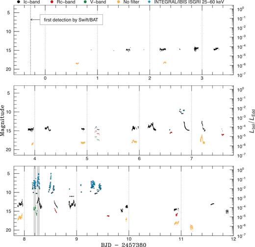
Overall light curves in the optical IC, RC and V bands and with no filter and in the X-ray 25–60 keV energy band of INTEGRAL IBIS/ISGRI monitoring during the 2015 December outburst in V404 Cyg. For clarity, the plotted magnitude for the unfiltered data is fainter by 2 mag than measured. The horizontal axis represents days from BJD 2457380. Here, LEdd is equal to 1.35 × 1039 (erg s−1). For visibility, only data points having horizontal error bars less than 1 h are plotted. The grey shadings represent the overlapped optical and X-ray observational periods.
3.2 Optical and X-ray correlation
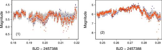
We found the simultaneous X-ray data with our optical data for two intervals: (1) during the day 8.18–8.22; and (2) during the day 8.246–8.292, where stochastic variations were observed (see the grey shadings in Fig. 1).7 The enlarged view of the intervals is displayed in Fig. 2. To examine the correlations between the optical and X-ray luminosities, we performed Spearman's rank tests on them in logarithmic scales and power-law regression assuming that they follow y = axb. Here, x and y denote the X-ray and optical (V- or IC-band) luminosities in linear scales, respectively. In these analyses, the completely simultaneous X-ray light curves to the optical ones were obtained by binning the INTEGRAL IBIS/ISGRI 25–60 keV light curves having a 1-s time bin size8 with the exposure times of the optical observations [30 s for interval (1) and 50 or 60 s for interval (2)] and calculating the weighted averaged flux in each bin. The optical data are corrected for interstellar extinction/absorption by assuming AV = 4 (Cardelli, Clayton & Mathis 1989; Casares et al. 1993). The results are summarized in Table 1. Both analyses have confirmed the correlated variations. The optical versus X-ray luminosity during the two time intervals is displayed in Fig. 3 with the regression equations.
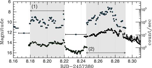
Simultaneous optical and X-ray light curves during intervals (1) the day 8.18–8.22 and (2) the day 8.246–8.292. Each of the intervals is ∼1 h long. The blue rhombuses, green squares and black circles represent the X-ray 25–60 keV, optical V-band and optical IC-band light curves. The optical flares are broader than the X-ray ones.
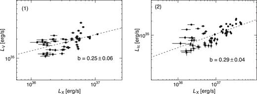
Optical and X-ray correlations during interval (1) on the day 8.18–8.22 (left-hand panel) and interval (2) on the day 8.246–8.292 (right-hand panel). The filled squares and circles represent the optical V-band and IC-band luminosities. The horizontal axes exhibit X-ray luminosity in the 25–60 keV energy band. The dashed lines represent the estimated power-law regression formulae for the relations between the optical and X-ray luminosities. The values of the power-law index (b) are also reported.
Results of Spearman's rank tests and power-law regression for the model of the form y = axb in time intervals (1) on the day 8.18–8.22 and (2) on the day 8.246–8.292.
| Intervals | a* | b* | ρ† | p-value‡ |
|---|---|---|---|---|
| (1) | 10(25.9 ± 2.076) | 0.255 (±0.0568) | 0.60 | 4.546 × 10⁻⁶ |
| (2) | 10(24.3 ± 1.431) | 0.290 (±0.0388) | 0.71 | 4.573 × 10⁻¹¹ |
| Intervals | a* | b* | ρ† | p-value‡ |
|---|---|---|---|---|
| (1) | 10(25.9 ± 2.076) | 0.255 (±0.0568) | 0.60 | 4.546 × 10⁻⁶ |
| (2) | 10(24.3 ± 1.431) | 0.290 (±0.0388) | 0.71 | 4.573 × 10⁻¹¹ |
Notes.*The values of degree of freedom of the regression in time intervals (1) and (2) are 49 and 61, respectively. As a result of t-tests of the regression coefficients, t-values of a and b were 12.495 (p < 2 × 10⁻¹⁶) and 4.487 (p = 4.37 × 10⁻⁵) for interval (1), and 16.988 (p < 2 × 10⁻¹⁶) and 7.472 (p = 3.57 × 10⁻¹⁰) for interval (2), respectively. These tests prove the estimated values of a and b to be statistically significant at the 1 per cent level. In addition, the values of F-tests were 20.84 (p = 4.371 × 10⁻⁵) for interval (1) and 55.83 (p = 3.567 × 10⁻¹⁰) for interval (2), respectively, and, hence, the assumption that a = b = 0 is abandoned.
†Spearman's correlation coefficients.
‡Null hypothesis probability of Spearman's correlation test. The null hypothesis is abandoned because the probability values are less than 0.01.
3.3 Bayesian time-delay analysis
We estimated time delays between our optical light curves and the INTEGRAL IBIS/ISGRI X-ray light curves with a time bin size of 5 s in the 25–60 keV energy band for interval (1) on the day 8.18–8.22 and interval (2) on the day 8.246–8.292 using a Bayesian method that was originally proposed to estimate time delays between gravitationally lensed stochastic light curves (Tak et al. 2016a).9 This method assumes that the irregularly sampled light curves are generated by a latent continuous-time damped random walk (DRW) process (Kelly, Bechtold & Siemiginowska 2009) and that one of the latent light curves is a shifted version of the other by the time lag in the horizontal axis and by the magnitude offset in the vertical axis (Pelt et al. 1994). The model also adopts heteroskedastic Gaussian measurement errors.
The DRW process is a stochastic process to describe a random walk with a tendency to move back towards a central location. This process is known to be appropriate for modelling accretion-type light variation such as the variability observed in active galactic nuclei (AGNs) because of its power-law-type power spectral density (Kelly et al. 2009; Kozłowski et al. 2010; MacLeod et al. 2010). This process is also suitable for modelling another accretion-type light variation in a black hole binary. This is because the power spectral densities of the X-ray light variations in V404 Cyg in the SCWs (162800020010, 162800030010, 162800040010 and 162800050010), including intervals (1) and (2), are well expressed by a power law (P ∝ f−Γ) with an index Γ of 1.6 ± 0.1, 1.5 ± 0.1, 1.6 ± 0.1 and 1.0 ± 0.2, respectively (see also Fig. S1 in the supplements to this paper).10
Our data, however, do not completely meet the second model assumption (i.e. one of the latent light curves is a parallel-shifted version of the other). This is because our optical light curves have smaller amplitudes than the X-ray ones and the origin of the optical light curves may be different from that of the X-ray ones unlike gravitationally lensed light curves as originally applied in Tak et al. (2016a). Thus, we scaled the X-ray light curve to the optical one using the results of the power-law regression (see Section 3.2 and Table 1) to meet the assumption before implementing the Bayesian method; we treated the scale change in the X-ray light curve as a known constant. The data sets for our analyses are displayed in Fig. 4. X-ray emission seems to be delayed to the optical emission when we focus on the sharp peaks with small measurement errors (e.g. around the day 8.209 in the upper panel and around the day 8.279 in the lower panel). The following time-lag estimations enable us to investigate the delay quantitatively.
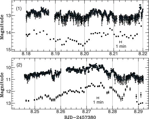
X-ray and optical data sets used for the time-delay estimates in interval (1) during the day 8.18–8.22 and interval (2) during the day 8.246–8.292. The X-ray light curves are rescaled by using the results of power-law regression described in Section 3.2. The rhombuses, squares and circles represent the X-ray light curves in the 25–60 keV energy band with a time bin size of 5 s after scaling, the optical V-band light curves and the optical IC-band light curves. For visibility, the X-ray magnitudes are offset by 7.7 for interval (1) and 4.7 for interval (2), respectively.
We used an r package, timedelay, which we made available to the public at CRAN,11 to implement the Bayesian model via a Markov chain Monte Carlo (MCMC) method; see Appendix A for details of the model, implementation and model checking. Fig. 5 exhibits the histogram of 300 000 posterior samples of the time lag between the optical and X-ray light curves for interval (1) in the left-hand panel and that for interval (2) in the right-hand panel. The estimation results are summarized in Table 2; the posterior median of the time delay for interval (1) was |$-45.3_{-1.1}^{+0.3}$| s and that for interval (2) was |$-33.1_{-0.2}^{+0.3}$| s, i.e. the X-ray variations were delayed to the optical variations by 45.3|$_{-1.1}^{+0.3}$| s for interval (1) and 33.1|$_{-0.2}^{+0.3}$| s for interval (2). The Gelman–Rubin convergence diagnostic statistics (Gelman & Rubin 1992) were 1.0004 and 1.0009 in intervals (1) and (2), respectively, close enough to unity. To check the consistency between different estimation methods, we compared our estimates with the results of a locally normalized discrete correlation function (LNDCF; Lehar et al. 1992). The LNDCF estimates averaged with a time bin size equal to 25.92 s showed |$-35_{-13}^{+13}$| s time lags in both intervals (1) and (2) (see also Fig. S2 in the supplements to this paper). Both Bayesian and LNDCF methods result in consistent estimates, considering the large uncertainties of the LNDCF estimates.

Posterior distributions of the time delays of the optical variations against the X-ray ones for interval (1) on the day 8.18–8.22 (left-hand panel) and interval (2) on the day 8.246–8.292 ( right-hand panel). The solid line indicates the posterior median of the time lag and the dashed lines represent the 68 per cent quantile-based interval. The time-lag estimate shown in each figure is the posterior median with a 68 per cent quantile-based interval. There are invisibly small modes near −30.5 and −25.8 s in the posterior distribution for interval (1) and near −48.1 s in that for interval (2), but we displayed only major modes.
Bayesian estimates of the time delays for interval (1) during the day 8.18–8.22 and interval (2) during the day 8.246–8.292. The 68 per cent interval indicates the quantile-based interval, and the 68 per cent Highest Posterior Density (HPD) interval represents the highest posterior density interval.
| Intervals | Mediana | 68 per cent interval | 68 per cent HPD interval |
|---|---|---|---|
| (1) | −45.4 s | (−46.5 s, −45.1 s) | (−45.6 s, −45.0 s) |
| (2) | −33.1 s | (−33.3 s, −32.8 s) | (−33.4 s, −32.9 s) |
| Intervals | Mediana | 68 per cent interval | 68 per cent HPD interval |
|---|---|---|---|
| (1) | −45.4 s | (−46.5 s, −45.1 s) | (−45.6 s, −45.0 s) |
| (2) | −33.1 s | (−33.3 s, −32.8 s) | (−33.4 s, −32.9 s) |
aWe report posterior medians because posterior means are not reliable indicators for the centre of a multimodal distribution. The posterior mode and median of time delays are identical up to three decimal places for interval (1). For interval (2), the posterior mode is −33.2 s.
4 DISCUSSION
4.1 Similarities between the two outbursts in 2015
Large-amplitude and short-term optical variations at low luminosity, which have good correlations with simultaneous X-ray variability, were observed during the two outbursts in 2015 in V404 Cyg (see also Kimura et al. 2016). This behaviour seems to be a common feature in every outburst of this system. Actually, violent optical variations with amplitudes of ∼1 mag on time-scales of days or minutes were also observed in the late stage of the 1989 outburst (Wagner et al. 1991). The amplitudes and time-scales of these optical variations and the occasional sudden dips in brightness during the December outburst were similar to those during the June outburst.
The overall trend of our optical light curves (a slow rise and rapid decay) in the December outburst was also similar to that in the June/July outburst, as Muñoz-Darias et al. (2017) already pointed out. This trend is different from the most common type of outburst in transient LMXBs (Chen, Shrader & Livio 1997). The slow rise could be the result of an inside-out outburst, which is considered to arise more frequently than an outside-in outburst in these objects (Lasota 2001, for a review). This possibility has already been suggested during the June outburst by estimating the disc radius at which an optical precursor was ignited (Bernardini et al. 2016a).
4.2 Differences in the short-term variability between the two outbursts in 2015
Although the morphologies of violent and rapid optical variations during the June and December outbursts resemble each other, the nature of these variations during the December outburst seems to be different from that during the June outburst. This is because we found X-ray variations lagging optical ones by ∼30–50 s for the two intervals during the December outburst (Section 3.3), which had not been detected during the June outburst. We consider whether two commonly known mechanisms of optical emission in X-ray binaries could explain the X-ray delays. They were expected to have been dominant at least at some time intervals during the June outburst. The first one is the reprocessing of X-ray irradiation from the inner disc (e.g. van Paradijs & McClintock 1994) and the second one is cyclo-synchrotron emission from magnetic flares, which would be related to a jet (e.g. Merloni, Di Matteo & Fabian 2000; Markoff, Falcke & Fender 2001). X-ray reprocessing will produce optical delays against X-rays on time-scales of tens of seconds (e.g. Hynes et al. 1998). On the other hand, cyclo-synchrotron radiation will induce very short time lags within 1 s between optical and X-ray variations, which are not consistent with the lags caused by X-ray reprocessing (e.g. Kanbach et al. 2001).12 We therefore conclude that these processes would fail to explain the observed X-ray delays in the December outburst. Even if we observed the expanding jet ejecta, the expected time lag was a ≳10 min optical delay (van der Laan 1966; Mirabel et al. 1998), as also discussed in the June outburst (Rodriguez et al. 2015; Martí et al. 2016). It is quite different from the X-ray delays that we estimated.
There are some other models including synchrotron radiation that have been developed to explain recently detected anticorrelated cross-correlation function signals with X-ray emission lagging the optical one by a few seconds and narrower optical autocorrelation functions to X-ray ones in several LMXBs (e.g. Malzac, Merloni & Fabian 2004; Durant et al. 2008; Gandhi et al. 2008; Veledina, Poutanen & Vurm 2011). The time-scales of the X-ray delays detected in this study, however, are inconsistent with the odd timing properties expected by these models as well as the smoother optical flares to the X-ray ones and the positive peaks at negative optical time lags in the DCFs (see also Figs 2 and S2).
There is some evidence to support that the effect of X-ray reprocessing and/or cyclo-synchrotron emission was weak. First, the estimated relation between the optical and X-ray luminosities in Section 3.2 was |$L_{\rm opt} \propto L_{\rm X}^{0.25\text{--}0.29}$| and this value disagrees with both that expected by standard disc reprocessing (|$L_{\rm V} \propto L_{\rm X}^{0.5}$|; van Paradijs & McClintock 1994) and that predicted by jet ejections plus X-ray irradiation (|$L_{\rm opt} \propto L_{\rm X}^{0.5-0.7}$|; Russell et al. 2006). Secondly, the optical-to-X-ray flux ratios in the December outburst (∼0.05 in the V band and ∼0.01 in the IC band) were smaller by a factor of 2–5 than those in the June outburst when X-ray reprocessing considerably dominated the optical flux. This would indicate that the effect of reprocessing was weaker in the December outburst than that in the June outburst. We suggest the reason is that the outer disc would be depleted due to ionization during the June outburst and/or the strong outflow discussed in Muñoz-Darias et al. (2016). On the other hand, in the June outburst, the outer disc is thought to have been optically thick (Kimura et al. 2016).
4.3 Time delay caused by propagation of mass accretion flow in the inner disc
We propose an interpretation that short-term variations of the mass-accretion rate in the outer disc (whose origin is still unknown) propagate to the inner disc via optical fluctuations, which will thereby prompt X-ray fluctuations. This then replaces the mechanisms discussed in the previous subsection as a possible origin of the delays. If the standard thin disc extends close to the central black hole, it will take longer for the observed delays to propagate in an accretion flow from the optical emission region to the X-ray emission region. This is because the speed of a propagating heating wave is proportional to the speed of sound (cs) in the standard disc (i.e. vf ∼ αcs; Meyer 1984). Here, α represents the viscous parameter. Thus, we consider the condition that the disc is composed of an optically thin flow as an advection-dominated accretion flow (ADAF) and a truncated geometrically thin standard disc. This picture was considered during the 2002 outburst in V4641 Sgr, another black hole transient LMXB, when a 7-min delay of the X-ray variations against the optical ones was detected at the fading stage (Uemura et al. 2004).
We assume that the thin standard disc extended to the transition radius (Rtr) and that there was the ADAF on the inside of the radius (e.g. Hameury et al. 1997). In the ADAF, the matter moves to the central object with a speed comparable to the free-fall velocity (vff) (vf ∼ αvff; Narayan & Yi 1995). If the optical fluctuations, which were triggered at a region close to the truncation radius, propagated to the central black hole via the accretion of mass flow on the free-fall time-scale in the ADAF, the transition radius is estimated to be ∼2.5–4.0× 10⁸ (cm) by using the above approximation for α = 0.01 (Sano, Inutsuka & Miyama 1998; Machida & Matsumoto 2003) and our estimates of X-ray delays. The estimated value of Rtr corresponds to ∼100–150rs. Here, rs (=2GM/c2) represents the Schwarzschild radius for a 9-M⊙ black hole. The estimated value is close to that of the inner disc radius derived through the SED analyses in the June outburst (see section 8 of Methods in Kimura et al. 2016). The region at the radius is, however, too hot to emit thermal optical photons predominantly; hence, the picture may be problematic. It is likely that the optical emission was non-thermal, as discussed in, for example, Uemura et al. (2002). In addition, the smaller amplitude of the optical variations can be explained by the presence of the optical continuum emission from the outer disc.
4.4 Testing possibilities of the origin of X-ray delays
An optically thin flow like an ADAF inside a truncated standard disc has been widely proposed as a possible scenario for the low/hard state in black hole X-ray binaries, although the interpretation remains under discussion (Remillard & McClintock 2006; Done, Gierliński & Kubota 2007; Belloni, Motta & Muñoz-Darias 2011, for a review). The average value of the bolometric luminosity during intervals (1) and (2), 0.03–0.1LEdd, is consistent with the observations in the low/hard state (Done & Gierliński 2003; Dunn et al. 2010), the existing theory (Yuan et al. 2007) and the 3D magnetohydrodynamics simulations (Machida, Nakamura & Matsumoto 2006; Oda et al. 2007). The spectral state was also reported to be the low/hard state during the day 8.15–10.32 (Motta et al. 2016); however, a detailed spectral analysis would be useful to test our interpretation since the peculiar X-ray spectral behaviour similar to that of an obscured AGN was found for some time intervals during the June outburst by Sanchez-Fernandez et al. (2017) and Motta et al. (2017). They suggested, on the basis of the spectral behaviour, that optically thick outflowing material would obscure substantial X-rays from the central part of V404 Cyg and that the intrinsic luminosity was close to the Eddington luminosity. This situation implies the existence of a slim disc; however, it would be difficult for short-term variability and time delays to coexist in this circumstance.13 Additionally, a slim disc itself would be difficult to maintain during the December outburst since the averaged X-ray flux during this outburst was much smaller than that during the June outburst.
5 CONCLUSIONS
We report on the photometric observations in the outburst of V404 Cyg from 2015 Decemberto 2016 January. Our main findings are summarized below:
The 2015 December outburst in V404 Cyg was very similar to the 2015 June–July outburst in the following two aspects. One is that violent and rapid optical variability with amplitudes of ∼2 mag on time-scales of ∼10 min to 3 h was observed at low luminosity. It is likely that this kind of variation is commonly seen in the outbursts, including the 1989 one, in this object. The other is that the trend of the overall light curves was a slow rise and rapid decay.
We detected an X-ray delay of ∼30–50 s against the optical emission in the two intervals during the December outburst, when the large-amplitude stochastic optical variations were observed at low average luminosity, ∼0.03–0.1LEdd. In addition, the relation between the optical and X-ray luminosities for these two intervals was |$L_{\rm opt} \propto L_{\rm X}^{0.25\text{--}0.29}$|. We suggest that the X-ray delay can be due to the propagation of mass accretion flow in an inner optically thin hot flow like an ADAF with a speed comparable to the free-fall velocity.
Acknowledgements
We acknowledge the variable star observations from the AAVSO International Database contributed by observers worldwide and used in this research. We also thank the INTEGRAL groups for making the products of the ToO data publicly available online at the INTEGRAL Science Data Centre. This work was financially supported by the Grant-in-Aid for Japan Society for the Promotion of Science Fellows for young researchers (MK) and the Grant-in-Aid ‘Initiative for High-Dimensional Data-Driven Science through Deepening of Sparse Modelling’ from the Ministry of Education, Culture, Sports, Science and Technology (MEXT) of Japan (25120007, TK). It was also partially supported by the RFBR grant 15-02-06178. We are thankful to many amateur observers for providing a lot of data used in this research. HT acknowledges partial support from the United States National Science Foundation under Grant Division of Mathematical Sciences 1127914 to the SAMSI. We give special thanks to Kaisey Mandel and David van Dyk for very helpful discussions. Yutaro Tachibana provided us with a code for calculations of LNDCFs. RDP gratefully acknowledges the use of the Las Cumbres Observatory Global Telescope Network. We are grateful to an anonymous referee for his/her helpful comments.
Here, Lbol is the bolometric luminosity.
The X-ray light curves are adaptively rebinned to achieve a signal-to-noise ratio (S/N) > 8 by the INTEGRAL team.
Although some of INTEGRAL Target of Opportunity (ToO) observations were performed during some other intervals, including the periods in which high-amplitude optical variations were observed (e.g. day 6.16–6.32, day 7.16–7.35 and day 8.84–8.96), the luminosity was very low at that time, and it was difficult to judge whether the optical and X-ray variability was correlated or not in those intervals due to the low S/N of the X-ray data.
The 1-s binned X-ray light curves were derived with the tool ii_light described in Section 2.2.
The 5-s binned X-ray light curves were derived with the tool ii_light described in Section 2.2.
We employed the powerspec software in the ftools xronos package from the lists of photons. The values of the ‘dtnt’ and ‘rebin’ parameters were 1 and −1.8 s, respectively. The Nyquist frequency of these observations was 0.5 Hz.
There may be a possibility that the very short time lag is not found because the observational data used in this work do not allow investigating millisecond-scale timing properties.
Sporadic mass accretion is unlikely to occur due to the high accretion rate in a slim disc. A variable absorber to cause the observed variability in the June outburst was suggested by Sanchez-Fernandez et al. (2017) and Motta et al. (2017), instead, but this condition would not produce time lags between optical and X-ray emission.
REFERENCES
SUPPORTING INFORMATION
Supplementary data are available at MNRAS online.
Table S1. Time-resolved CCD photometry carried out by the Variable Star Network collaboration team (Kato et al. 2004) at 17 sites.
Table S2. Log of our photometric observations in the V, RC and IC bands and with a clear filter.
Table S3. List of comparison stars.
Figure S1. PSDs of the X-ray light curves in the SCWs including interval (1) during the day 8.18–8.22 and interval (2) during the day 8.246–8.292.
Figure S2. Estimated LNDCFs in interval (1) during the day 8.18–8.22 and interval (2) during the day 8.246–8.292.
Please note: Oxford University Press is not responsible for the content or functionality of any supporting materials supplied by the authors. Any queries (other than missing material) should be directed to the corresponding author for the article.
APPENDIX A: DETAILS OF THE BAYESIAN MODEL, IMPLEMENTATION AND MODEL CHECKING
Our full posterior density, |$\pi (\boldsymbol {X}(\boldsymbol {t}^{\Delta }), \Delta , \beta _0, \mu , \sigma ^2, \tau \mid \boldsymbol {x}, \boldsymbol {y})$|, is proportional to the multiplication of the probability density functions, whose distributions are specified in (A1), (A4), (A5) and (A6). We use a Metropolis–Hastings within the Gibbs sampler (Tierney 1994) to sample the full posterior distribution of the model parameters; see section 3 of Tak et al. (2016a) for details of this sampler. To improve the convergence of the MCMC for Δ in the presence of multimodality, we adopt a repelling–attracting Metropolis algorithm (Tak, Meng & van Dyk 2016b).
We initialize three Markov chains near the dominating mode for each time interval, running for 150 000 iterations; we discard the first 50 000 as burn-in iterations. The proposal scale of Δ (delta.proposal.scale in Table A1) is set to produce the largest acceptance rate while making the Markov chains jump frequently between the modes identified by the profile likelihood. The average acceptance rate of the time lag is 0.216 for interval (1) and 0.186 for interval (2).
Initial values of the parameters for each of three Markov chains used in the function bayesian of the r package timedelay for interval (1) during the day 8.18–8.22 and interval (2) during the day 8.246–8.292.
| Names of parameters | (1) | (2) |
|---|---|---|
| theta.ini (μ, σ, τ)|$^{^a}$| | (5.30, 100, 0.01) | (5.72, 100, 0.01) |
| (5.30, 10, 0.1) | (5.72, 10, 0.1) | |
| (5.30, 1, 1) | (5.72, 1, 1) | |
| delta.ini|$^{^b}$| | −0.000 582 7546 | −0.000 440 5093 |
| −0.000 524 8843 | −0.000 382 6389 | |
| −0.000 467 0139 | −0.000 324 7685 | |
| delta.uniform.range|$^{^c}$| | (−0.04, 0.04) | (−0.046, 0.046) |
| delta.proposal.scale|$^{^d}$| | 0.000 05 | 0.000 05 |
| tau.proposal.scale|$^{^e}$| | 1 | 1 |
| tau.prior.shape|$^{^f}$| | 1 | 1 |
| tau.prior.scaleg | 2/107 | 2/107 |
| sigma.prior.shape|$^{^h}$| | 1 | 1 |
| sigma.prior.scale|$^{^i}$| | 1 | 1 |
| adaptive.delta|$^{^j}$| | False | False |
| multimodality|$^{^k}$| | True | True |
| micro|$^{^l}$| | 0 | 0 |
Notes.a Initial values of the DRW parameters. Unit of magnitudes in μ and σ. Unit of days in τ.
bInitial value of the delay time for MCMC used in three Markov chains. Unit of days.
cRange of uniform prior distribution of the time delay Δ. Unit of days.
dProposal scale of the Metropolis step for the time delay Δ. Unit of days.
eProposal scale of the Metropolis–Hastings step for log (τ). Units of τ are days.
fShape parameter of Inverse-Gamma hyper-prior distribution for τ.
gScale parameter of Inverse-Gamma hyper-prior distribution for τ.
hShape parameter of Inverse-Gamma hyper-prior distribution for σ2.
iScale parameter of Inverse-Gamma hyper-prior distribution for σ2.
jWe do not use the adaptive MCMC for the time delay Δ in the presence of multimodality because the adaptation may occur at a local mode.
kWe use a repelling–attracting Metropolis algorithm to sample the time delay Δ.
lThe order of a polynomial regression model. We do not consider the effect of microlensing in the case of V404 Cyg.
We visually checked our estimates, shifting the optical light curves by the posterior medians of Δ and β0 in Fig. A1; the fitted model matches the fluctuations of the two light curves well. We also conducted a model checking by plotting the posterior sample of the latent curve in grey; the grey areas encompass most of the observed light curves, which shows how well the fitted model predicts the observed data. A sensitivity analysis, though not shown here, exhibits that our inferential results in Table 2 are robust to changing the scale parameters in the inverse Gamma distributions of σ2 and τ.
The X-ray light curves are denoted by orange squares, the optical light curves are denoted by blue circles and the posterior samples of latent light curves at intervals of 300 iterations are denoted by grey circles in interval (1) on the day 8.18–8.22 (left-hand panel) and interval (2) on the day 8.246–8.292 (right-hand panel). Each optical light curve is shifted by the posterior mode of the time lag in the horizontal axis and by that of the magnitude offset in the vertical axis. The fitted model makes a good match of the fluctuations of the two light curves. The grey areas are encompassing most of the light curves, meaning that the fitted model describes the observed data well.
