


Abstract
To fully understand cosmic black hole growth, we need to constrain the population of heavily obscured active galactic nuclei (AGNs) at the peak of cosmic black hole growth (z ∼1–3). Sources with obscuring column densities higher than 1024 atoms cm−2, called Compton-thick (CT) AGNs, can be identified by excess X-ray emission at ∼20–30 keV, called the ‘Compton hump’. We apply the recently developed Spectral Curvature (SC) method to high-redshift AGNs (2 < z < 5) detected with Chandra. This method parametrizes the characteristic ‘Compton hump’ feature cosmologically redshifted into the X-ray band at observed energies <10 keV. We find good agreement in CT AGNs found using the SC method, and bright sources fit using their full spectrum with X-ray spectroscopy. In the Chandra Deep Field-South, we measure a CT fraction of 17|$^{+19}_{-11}\hbox{\,per\,cent}$| (3/17) for sources with observed luminosity >5 × 1043erg s−1. In the Cosmological Evolution Survey (COSMOS), we find an observed CT fraction of |$15^{+4}_{-3}\hbox{\,per\,cent}$| (40/272) or 32 ± 11 per cent when corrected for the survey sensitivity. When comparing to low redshift AGNs with similar X-ray luminosities, our results imply that the CT AGN fraction is consistent with having no redshift evolution. Finally, we provide SC equations that can be used to find high-redshift CT AGNs (z > 1) for current (XMM–Newton) and future (eROSITA and ATHENA) X-ray missions.
1 INTRODUCTION
Active galactic nuclei (AGNs) are believed to be powered during accretion episodes in which matter from galactic scales is accreted on to the central supermassive black hole (SMBH, e.g. Soltan 1982; Marconi et al. 2004; Merloni, Rudnick & Di Matteo 2006). During these accretion phases, periods of maximal growth occur in the SMBH (e.g. Ferrarese & Ford 2005; Johnson et al. 2013). Due to the large amount of matter involved during the accretion of a SMBH, a significant fraction of AGNs is obscured from sight (e.g. Balokovic et al. 2014; Brightman et al. 2014). Thus, to understand the evolution history of all the SMBHs through cosmic time, we need a complete census of the AGN population including the heavily obscured sources (e.g. Treister, Urry & Virani 2009; Ueda et al. 2014; Buchner et al. 2015; Ricci et al. 2015). The capability of the X-ray emission at energies >10 keV to penetrate obscuring matter makes them one of the best tools to study obscured AGNs (Risaliti, Maiolino & Salvati 1999; Barger et al. 2003; Georgantopoulos & Akylas 2009). The detection of AGNs can, however, become very challenging when the absorption reaches Compton-thick (CT) levels (Georgantopoulos et al. 2010; Lanzuisi et al. 2015; Brandt & Alexander 2015). We define an AGN as CT when it is surrounded by obscuring material with column density on the line of sight larger than the inverse Thomson cross-section (|$\mathrm{N_H \ge \sigma _T^{-1} \approx 1.5 \times 10^{24}\, atoms\, cm^{-2},}$| Comastri 2016).
The study of highly obscured sources, such as CT AGNs, is crucial to achieve a complete census of the accreting SMBH population and to obtain an unbiased X-ray luminosity function (e.g. Fabian & Iwasawa 1999; Alexander 2007; Georgakakis et al. 2015). Gilli, Comastri & Hasinger (2007) found that to explain the cosmic X-ray background (XRB) peak at ∼30 keV, the fraction of CT AGNs must be equivalent to the fraction of moderately obscured sources (21 < log(NH) < 24). Their results agree with Fiore et al. (2008). Daddi et al. (2007) studied the population at z ∼ 2 showing an excess in the mid-IR wavelength suggesting a space density of CT AGNs of ∼2.6 × 10⁻⁴ Mpc−3. However, they found that even if the population of CT AGNs has a large space density, the CT contribution to the still missing XRB is of the order of 10 per cent–25 per cent. This result is consistent with what has been found by Treister et al. (2009). The analysis of the hard X-ray luminosity function from Ueda et al. (2014) using X-ray data from Swift/BAT, MAXI, ASCA, XMM–Newton, Chandra and ROSAT reveals that the number of sources with column density between log(NH) = 24–25 must be equal to the number of sources with log(NH) = 23–24 to explain the cosmic XRB emission at 20 keV. This result is similar to what has been found by Gilli et al. (2007). X-ray spectral analysis of the 4 Ms Chandra Deep Field-South (CDF-S) by Brightman & Ueda (2012) using spectral models from Brightman & Nandra (2011) showed a CT fraction in the nearby Universe of ∼20 per cent growing to ∼40 per cent at redshift z = 1–4. However, Buchner et al. (2015) combined deep and wide-area Chandra and XMM–Newton X-ray surveys, and they did not find any evidence of the redshift evolution of the CT fraction, which they found to be |$38^{+8}_{-7}\hbox{\,per\,cent}$| on a redshift range from 0.5 to 2. This could be explained by the difference in the analysed luminosity ranges as the sample in Buchner et al. (2015) includes sources with X-ray luminosities down to 1043.2 erg s−1. Ricci et al. (2015) found the CT fraction to be luminosity dependent with 32 ± 7 per cent at luminosities log(L14-195keV) = 40–43.7, while only 21 ± 5 per cent at higher luminosities log(L14-195keV) = 43.7–46. This result is similar to what found by Civano et al. (2015), who performed an analysis of the Cosmological Evolution Survey (COSMOS) field with NuSTAR, finding a CT fraction between 13 per cent and 20 per cent at redshift z = 0.04–2.5. However, the result of Ricci et al. (2015) is corrected from bias, while the fraction in Civano et al. (2015) is not. We note that some studies have suggested that most of them ‘missing’ XRB is expected to be produced by objects with intrinsic luminosity smaller than 1044 erg s−1 and z < 1 (Gilli 2013). In summary, despite extensive research, there is still considerable disagreement about the fraction of CT AGNs and their contribution to the XRB particularly at high redshift.
In CT AGNs, the majority (>95 per cent) of the hard X-ray (2–10 keV) emission is obscured/scattered (Risaliti et al. 1999; Matt et al. 2000). The X-ray spectra, however, feature a prominent Fe Kα emission line with large equivalent width, EW > 1 keV (e.g. Nandra et al. 1997; Reynolds 1999; Vignali & Comastri 2002; Liu et al. 2016), and the Compton hump, peaking at ∼20–30 keV (Krolik 1999; Nandra 2006). The spectral curvature (SC) method was developed by Koss et al. (2016), to identify nearby (z < 0.03) CT AGN candidates in Swift/BAT and NuSTAR using the (>10 keV) SC. The sensitivity of NuSTAR is 1 × 10⁻¹⁴ erg cm−2 s−1 in the 10–30 keV range (Harrison et al. 2013), while Swift/BAT has a sensitivity of 10−11 erg cm−2 s−1 in the deepest all sky maps (Krimm et al. 2013). Thus, both instruments select relatively bright sources compared to the faint high-redshift AGNs detected by Chandra. The CDF-S, which is the deepest survey of the Chandra X-ray observatory, has a flux limit of 5.5 × 10⁻¹⁷ erg cm−2 s−1 in the 2–10 keV energy range (Xue et al. 2011). Hence, it can detect much fainter sources than NuSTAR such as high-redshift CT AGNs.
In this article, we extend the SC method to high-redshift (z > 2) AGNs where the rest-frame Compton hump feature can be observed with Chandra. In Section 2, we describe our simulations to define the method for Chandra, in Section 3, we apply it to Chandra fields, and finally in Section 4, we discuss implications. Throughout this work, we adopt Ωm = 0.27, |$\Omega _\Lambda$| = 0.73 and H0 = 71 km s−1 Mpc−1. Errors are quoted at the 90 per cent confidence level unless otherwise specified.
2 THE SPECTRAL CURVATURE METHOD
To estimate the likelihood of an X-ray source to be CT, the SC method uses the distinctive spectral shape of CT AGNs at energies higher than 10 keV. In this work, we follow the technique used for low-redshift sources (e.g. Koss et al. 2016), where we model an unobscured source with a power law of Γ = 1.9, and a heavily CT source as an AGN with line-of-sight column densities of NH = 5 × 1024 cm−2, using the MYtorusspectral models from Yaqoob (2012). We choose the threshold at column density NH = 5 × 1024 cm−2 to be consistent with Koss et al. (2016). The SC equation is modelled so that an unobscured source has an SC value of zero, while a heavily CT AGN has an SC value of one.
As a first step, we simulated the SC of obscured AGNs at high redshift with the xspec (version 12.9.0) fakeit tool. Fig. 1, left-hand panel, shows how the SC measure increases with higher column density. For simplicity, we assume NH = 1024 cm−2 as the lower limit of column density for CT AGNs. The coefficients of the SC equation are defined using weighted and averaged counts of simulated unobscured and CT sources in three different energy ranges divided by the total counts in the entire range (8–24 keV rest frame) (Fig. 1, right-hand panel). Finally, since we worked with observations of objects at redshift z > 2, the corresponding energy ranges in the observed frame are [8–12]/(1 + z), [12–16]/(1 + z) and [16–24]/(1 + z) keV.
![Left-hand panel: CT AGNs at redshift z = 2 simulated using the MYTorus model compared to an unobscured power law with Γ = 1.9. As NH increase from 1019 atoms−2 to 5 × 1024 atoms−2, the curvature of the observed radiation increases. At redshift z > 2, the peak of the Compton hump is at rest-frame energies smaller than 8 keV and can be observed with Chandra. Right-hand panel: Chandra number of counts for the same simulated sources at z = 2 normalized by the total number of counts of the power-law source in the full energy band [8–24]/(1 + z) keV. The vertical dashed lines show the three energy ranges [8–12]/(1 + z), [12–16]/(1 + z) and [16–24]/(1 + z) keV. For energies above 4.5 keV (observed frame), the CT sources show an excess compared to the rate of an unobscured source. At energies below 4.5 keV, CT sources show a decrement.](https://oup.silverchair-cdn.com/oup/backfile/Content_public/Journal/mnras/471/1/10.1093_mnras_stx1561/1/m_stx1561fig1.jpeg?Expires=1750829708&Signature=aw0T3GHFegVr1mfC1d3NdB396~YiEo~wzPhijvEKg~9bPiQy3o8tp26pUH33dLBRBYQbFqX4MBdbvOD~ukK725OzS-yLrYADhUwNspORoFzFwS9ujgQRtg7rCOgtolQCkyWl0wYnheCXAMyeYSUuIaJOv8AGrjqykB7DpGmY9I-M-g95pSnSduMjIF-kePA~MpdHwdd128u6OMszmfSecjQ-jAIg9CFIDjP2wvY89RxUju55TrEEEN0rrNoPiTL3iZ-HhTqjZRYzwWQuu5eyRgqAMtMvmxkzC8CCQwklJl7mL-hYm0DGSh7w0dmPxn-hWUxWzP1aOtCqxaoUbGIbFg__&Key-Pair-Id=APKAIE5G5CRDK6RD3PGA)
Left-hand panel: CT AGNs at redshift z = 2 simulated using the MYTorus model compared to an unobscured power law with Γ = 1.9. As NH increase from 1019 atoms−2 to 5 × 1024 atoms−2, the curvature of the observed radiation increases. At redshift z > 2, the peak of the Compton hump is at rest-frame energies smaller than 8 keV and can be observed with Chandra. Right-hand panel: Chandra number of counts for the same simulated sources at z = 2 normalized by the total number of counts of the power-law source in the full energy band [8–24]/(1 + z) keV. The vertical dashed lines show the three energy ranges [8–12]/(1 + z), [12–16]/(1 + z) and [16–24]/(1 + z) keV. For energies above 4.5 keV (observed frame), the CT sources show an excess compared to the rate of an unobscured source. At energies below 4.5 keV, CT sources show a decrement.
2.1 The spectral curvature equation
We first consider the importance of energy-dependent vignetting and point spread function degradation with off-axis angle. We tested the behaviour of the SC equations for off-axis sources by simulating spectra of unobscured, obscured and CT AGNs at constant redshift z = 2, exposure time (4 Ms) and intrinsic luminosity of 5 × 1044 erg s−1, using response files corresponding to different off-axis positions. The response files at different off-axis angles are obtained using the ciao 4.9 tools mkacisrmf and mkarf.1 We averaged over 100 simulations to reduce the effect of Poisson noise. The coefficients of the SC equation show very little dependence on the off-axis position of the source in Chandra (Fig. 4). Nevertheless, we note that above 8-arcmin off-axis distance, the large PSF significantly reduces sensitivity in Chandra. On the other hand, the SC coefficients show a strong redshift dependency that can be corrected for using an additional redshift correction factor.
2.1.1 Redshift dependence
After applying the method developed in Koss et al. (2016) to the redshift interval from 2 to 5, the SC values and the thresholds between CT and non-CT sources depend significantly on the redshift. We therefore add a redshift parameter to the SC equation, so that the new input variables are the normalized counts in the three energy ranges (A, B and C) and include the change with redshift.
We tested the SC method on a sample of simulated X-ray spectra with different column densities and luminosities. The integration time for the simulation is set to 4 Ms, this determines a limit on the maximum number of counts obtained. From Figs 2 and 3, we observe that the method successfully distinguishes between simulated sources with column densities below NH = 1024 cm−2 and CT sources. Moreover, from Fig. 3, we can estimate where the SC method is less reliable for sources with very few counts due to the large error bars. We note that between 10 and 70 counts, the SC method presents large uncertainties that could make uncertain the classification for single sources, however, the population can be studied in aggregate. Moreover, the method is less sensitive to sources with column densities exceeding NH = 1025 cm−2, since at these column densities, the Compton hump intensity is reduced by Compton scattering. Thus, the SC method is better suitable for transmission-dominated (NH < 1025 cm−2) CT AGNs.
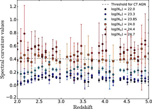
Normalized SC values of simulated sources versus the redshift. The SC method selects sources with column densities above 1024 cm−2 as CT AGNs. Thus, the SC method successfully distinguishes CT sources from merely obscured AGNs.
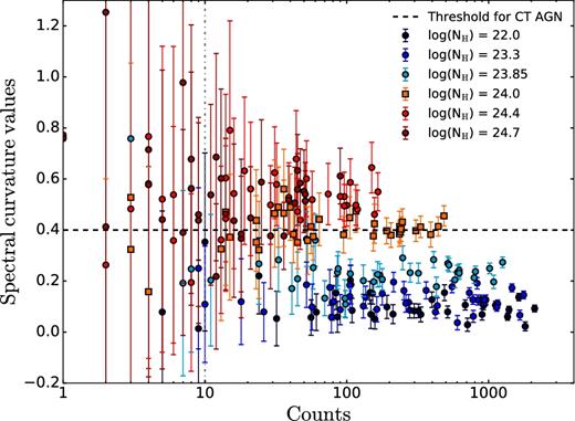
Evolution of the SC values as function of column density and counts in the full energy range. Note that for smaller number of counts, the error bars become larger. For less than 10 counts in the full energy range, the SC value is unreliable. The spectra of non-CT and CT sources are simulated using the fakeit tool of xspec by constant exposure time of 4 Ms, this determines the upper limit in the number of counts of the spectra.
3 SAMPLE AND DATA ANALYSIS
We applied the SC method to deep Chandra observations. Thanks to the high sensitivity of Chandra, we can find CT candidates even at redshift higher than 2. The deepest Chandra surveys are the CDF-S and the COSMOS legacy survey (Fig. 5).
3.1 CDF-S
The CDF-S has an on-axis flux limits reaches 3.2 × 10⁻¹⁷, 9.1 × 10⁻¹⁸ and 5.5 × 10⁻¹⁷ erg cm−2 s−1 in the energy ranges 0.5–8, 0.5–2 and 2–8 keV, respectively (Xue et al. 2011; Fig. 5). For this catalogue, the reduced spectra have not been made public. Thus, we applied the SC method on the 4-Ms merged event file.2 The coordinates and redshifts that we used can be found in the catalogue of Xue et al. (2011).
We excluded from the analysis the sources with angular distance greater than 8.7 arcmin from the image centre (Fig. 4 ) because of their significantly reduced sensitivity and exposure time. We extracted the net number of counts and the error on it using the ciao tool dmextract. We extracted the net counts in the three energy ranges [8–12]/(1 + z), [12–16]/(1 + z) and [16–24]/(1 + z) keV. The error on the net counts is calculated directly with dmextract using the Gehrels statistic (Gehrels 1986). The flux limit for the CDF-S is calculated for unobscured sources. Hence, the survey may miss sources with very high level of obscuration that fall below the detection limit, for example the reflection-dominated CT AGNs (NH > 1 × 1025 cm−2).
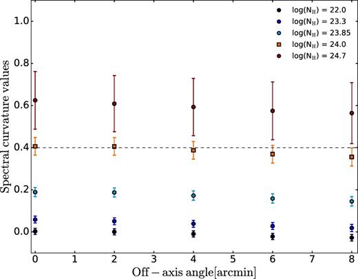
Spectral curvature values as function of the off-axis position for simulated AGNs with different column densities NH, redshift z = 2 and with intrinsic luminosity of 5 × 1044 erg s−1. The deviations in the SC values due to the off-axis position are small compared to the error bars.
3.2 Cosmos
The Chandra COSMOS Legacy Survey covers 2.2 deg2 of the COSMOS field to a flux limit of 2.2 × 10⁻¹⁶, 1.5 × 10⁻¹⁵ and 8.9 × 10⁻¹⁶ erg cm−2 s−1 in the 0.5–2, 2–10 and 0.5–10 keV bands, respectively (Civano et al. 2016; Fig. 5). The depth of the flux and the relatively large area of the COSMOS-Legacy survey are going to remain unrivaled until the advent of ATHENA (Civano et al. 2016).
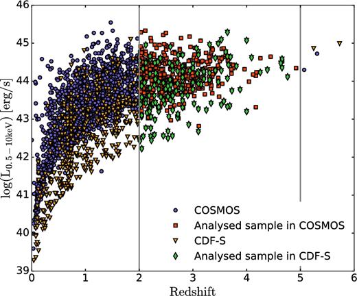
Luminosity in the 0.5–10 keV range compared with the redshift. The black dashed line shows the flux limit in the full energy range. The squared points indicate the sources taken into account in this work. Data from Marchesi et al. (2016a).
We used the X-ray spectra of the sources in the COSMOS-legacy survey from Civano et al. (2016). For the purposes of our analysis, for each source in the Chandra COSMOS-Legacy sample we used xspec (version 12.9.0) to estimate the number of counts in the energy intervals [8–12]/(1 + z), [12–16]/(1 + z) and [16–24]/(1 + z) keV. The number of counts in the energy range is calculated by multiplying the count rate (obtained by calling the attribute rate of xspec.spectrum) with the exposure time. To determine the errors on the number of counts, we applied Gehrels statistic (Gehrels 1986). The exposure times of our sample range from 40 to 250 ks. We did not exclude sources at largest off-axis angles. The flux limit for the COSMOS survey is calculated for unobscured source. Therefore, highly obscured sources are likely to be missed from the survey.
4 RESULTS
4.1 CDF-S
By applying the SC method on 17 sources with luminosity higher than 5 × 1043 erg s−1 and with spectroscopic redshift in the 4 Ms CDF-S (see Table 1), we obtained three CT candidates (the three blue dots above the CT threshold line in Fig. 6). Of these, only the one at redshift 3.66 has net number of counts higher than 100 (see Fig. 6, middle source above the threshold). The source above the CT threshold at redshift 4.67 has coordinates RA = 3:32:29.27, Dec. = −27:56:19.8 (XID403), and has been proposed as a CT candidate in Gilli et al. (2011). The SC value could be verified by applying the SC method to the coming 7-Ms CDF-S survey, which will have tighter limits and smaller uncertainties.
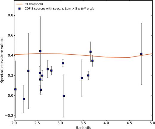
CDF-S spectral curvature values for sources with spectroscopic redshift. The red line shows the threshold between non-CT and CT AGNs. The sources we show here are enclosed in a region with radius of 8.7 arcmin from the field centre to avoid the sources with extremely large PSF. To take into account only the SC values with smaller error bars, we apply the SC method only on sources with luminosity higher than 5 × 1043 erg s−1. The source at redshift z = 4.67 has been proposed as a CT AGNs by Gilli et al. (2011). The SC method selects this source as a CT candidate but still with a large error bar.
SC values for the analysed sample in the CDF-S.
| XIDa | zb | Soft ctsc | Mid ctsd | Hard ctse | Total ctsf | SCg | CT candidate |
|---|---|---|---|---|---|---|---|
| 710 | 2.03 | 45 ± 10 | 17 ± 10 | 16 ± 10 | 77 ± 17 | 0.06 ± 0.29 | |
| 369 | 2.21 | 101 ± 17 | 54 ± 13 | 25 ± 13 | 180 ± 25 | −0.03 ± 0.14 | |
| 20 | 2.31 | 21 ± 9 | 7 ± 7 | 13 ± 8 | 42 ± 14 | 0.25 ± 0.38 | |
| 188 | 2.56 | 127 ± 14 | 90 ± 13 | 88 ± 13 | 306 ± 23 | 0.23 ± 0.07 | |
| 93 | 2.57 | 44 ± 10 | 31 ± 9 | 25 ± 9 | 100 ± 16 | 0.16 ± 0.14 | |
| 294 | 2.57 | 17 ± 8 | 4 ± 7 | 20 ± 8 | 41 ± 13 | 0.44 ± 0.34 | Yes |
| 687 | 2.58 | 268 ± 22 | 167 ± 18 | 98 ± 16 | 533 ± 33 | 0.06 ± 0.05 | |
| 137 | 2.61 | 147 ± 14 | 109 ± 12 | 95 ± 12 | 351 ± 22 | 0.20 ± 0.05 | |
| 86 | 2.73 | 89 ± 15 | 55 ± 12 | 74 ± 13 | 218 ± 23 | 0.26 ± 0.09 | |
| 149 | 2.81 | 197 ± 17 | 172 ± 15 | 168 ± 16 | 537 ± 28 | 0.25 ± 0.04 | |
| 546 | 3.06 | 201 ± 16 | 185 ± 15 | 247 ± 17 | 633 ± 28 | 0.32 ± 0.04 | |
| 674 | 3.08 | 26 ± 8 | 11 ± 7 | 7 ± 8 | 45 ± 13 | −0.00 ± 0.21 | |
| 588 | 3.47 | 27 ± 8 | 5 ± 6 | 18 ± 8 | 50 ± 13 | 0.18 ± 0.18 | |
| 563 | 3.61 | 162 ± 15 | 89 ± 12 | 127 ± 14 | 378 ± 23 | 0.20 ± 0.04 | |
| 262 | 3.66 | 24 ± 7 | 33 ± 8 | 60 ± 10 | 117 ± 14 | 0.44 ± 0.10 | Yes |
| 412 | 3.7 | 65 ± 10 | 74 ± 10 | 108 ± 12 | 247 ± 18 | 0.35 ± 0.06 | |
| 403 | 4.76 | 9 ± 5 | 4 ± 4 | 12 ± 5 | 24 ± 8 | 0.42 ± 0.31 | Yes |
Notes.aIdentification number of the source in the 4-Ms CDF-S (Xue et al. 2011).
bSpectroscopic redshift from Xue et al. (2011).
cNumber of counts in the soft energy range [8–12]/(1 + z) keV.
dNumber of counts in the mid energy range [12–16]/(1 + z) keV.
eNumber of counts in the hard energy range [16–24]/(1 + z) keV.
fNumber of counts in the total energy range [8–24]/(1 + z) keV.
gMeasured spectral curvature values.
Constraining our analysis to sources with spectroscopic redshift, the fraction of CT AGNs selected in the CDF-S is 17|$^{+18.6}_{-11.0}\hbox{\,per\,cent}$| (3/17 sources with spectroscopic redshift), assuming binomial statistics with 90 per cent of confidence. The value we obtain is similar to what was found by Koss et al. (2016). However, the sample analysed in the CDF-S is small. To have more reliable constraints on the CT AGN populations, we will focus on the larger sample obtained from the COSMOS-legacy survey.
4.2 Cosmos
We calculated the SC values for the sources in the COSMOS-legacy survey between redshift 2 and 5 (Fig. 7). The redshift and the column densities of the COSMOS sources can be found in the Marchesi et al. (2016a) catalogue. The NH values therein are calculated from hardness ratio ratios and redshifts. In total, we applied the method to 272 sources (see Table 2), 158 catalogued as Seyfert 1 (i.e. unobscured AGNs showing both broad and narrow optical emission lines) and 68 catalogued as Seyfert 2 (i.e. obscured AGNs showing only narrow optical emission lines).
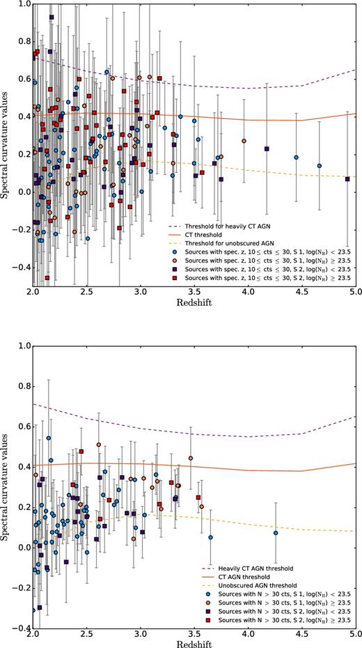
Top panel: The fraction of sources with NH < 23.5 selected as CT candidates is 8.6|$^{+4.3}_{-3.2}\hbox{\,per\,cent}$|. Of the sources (120) catalogued with column density log(NH) ≥ 23.5, 54 are catalogued as Seyfert 1. The fraction of CT candidates selected for this NH range are |$22.5^{+6.7}_{-5.7}\hbox{\,per\,cent}$|. Bottom panel: Same as above but showing only the detected sources with more than 30 counts. 80 per cent of the CT candidates (4/5 sources) agree with the spectral measurements.
SC values for the analysed sample in the COSMOS legacy survey. This table is available in its entirety in a machine-readable form in the online journal. A portion is shown here for guidance regarding its form and content.
| IDa | zb | Soft ctsc | Mid ctsd | Hard ctse | Total ctsf | SCg | CT candidate | |$N_{\rm H}^{h}$| [1022 atoms cm−2] | |$N_{\rm H}^{i}$| [1022 atoms/cm2] |
|---|---|---|---|---|---|---|---|---|---|
| Lid_471 | 2.0 | 7 ± 4 | 8 ± 4 | 6 ± 3 | 23 ± 6 | 0.41 ± 0.38 | Yes | 18.8 | 16.10 |
| Lid_1026 | 2.00 | 10 ± 4 | 9 ± 4 | 5 ± 3 | 25 ± 6 | 0.23 ± 0.33 | 25.3 | 2.67 | |
| Lid_249 | 2.00 | 24 ± 6 | 6 ± 3 | 2 ± 3 | 33 ± 6 | −0.31 ± 0.21 | 0 | 4.22 | |
| Cid_545 | 2.01 | 14 ± 5 | 6 ± 3 | 2 ± 3 | 23 ± 6 | −0.16 ± 0.32 | 0 | 9.95 | |
| Lid_635 | 2.01 | 6 ± 3 | 2 ± 3 | 7 ± 4 | 16 ± 5 | 0.71 ± 0.6 | Yes | 0 | 3.43 |
| Cid_1512 | 2.02 | 9 ± 4 | 0 ± 2 | 11 ± 4 | 20 ± 5 | 0.73 ± 0.56 | Yes | 56.4 | 56.40 |
| Cid_282 | 2.02 | 13 ± 4 | 11 ± 4 | 6 ± 3 | 30 ± 6 | 0.18 ± 0.28 | 0 | 0.79 | |
| Cid_351 | 2.02 | 54 ± 8 | 20 ± 5 | 11 ± 4 | 86 ± 10 | −0.11 ± 0.13 | 0 | 2.41 | |
| Cid_424 | 2.02 | 8 ± 4 | 6 ± 3 | 7 ± 3 | 22 ± 5 | 0.46 ± 0.41 | Yes | 5.65 | 0.79 |
Notes.aIdentification number of the source, from the COSMOS legacy survey (Marchesi et al. 2016a).
bSpectroscopic redshift from Marchesi et al. (2016a).
cNumber of counts in the soft energy range [8–12]/(1 + z) keV.
dNumber of counts in the mid energy range [12–16]/(1 + z) keV.
eNumber of counts in the hard energy range [16–24]/(1 + z) keV.
fNumber of counts in the total energy range [8–24]/(1 + z) keV.
gMeasured Spectral Curvature values.
hColumn density from Marchesi et al. (2016a) estimated using a hardness ratio.
iColumn density estimated from Marchesi et al. (2016b) spectral fitting.
We found that 14.5 per cent (40/272) sources are selected as CT AGNs. The SC method selects no CT candidate at redshift z > 3.5, primarily due to the much smaller number of sources in the survey and their faintness. If we restrict the luminosity to LX > 1044 erg s−1 to avoid biases due to the flux limit of the COSMOS survey, we find that the fraction of CT AGNs is 8.9 per cent (13/145). We chose to apply this luminosity cut, since we are comparing the obtained CT fraction in different redshift bins over a specific luminosity range so that it can be compared to other published studies (e.g. Ricci et al. 2015) and because of the low statistical significance of the SC for sources just above the detection limit. The focus on higher luminosity AGNs in this paper will likely exclude some number of absorbed AGNs because of the well-known anti-correlation between fraction of absorbed AGNs and luminosity (e.g. Hasinger 2008). Considering the total sample of CT candidates (without luminosity cuts), 18/40 (45 per cent) are described as Seyfert 1 in the catalogue. This means that 11.4 per cent of sources that are considered unobscured in the optical is selected as CT AGN candidates. On the other hand, 22 sources are selected from the 68 catalogued as Seyfert 2. This means that the 32.4 per cent of the Seyfert 2 is selected as CT. We also have to consider the possibility that the classification of Seyfert 1 and Seyfert 2 in the Marchesi et al. (2016a) catalogue might have some uncertainties. Additionally, the definitions of Seyfert 1 and Seyfert 2 are based on optical spectra, and X-ray (unobscured versus obscured) schemes of classification do not always agree (e.g. Burtscher et al. 2016). To explore this possibility, we examined the SC values of the COSMOS sample for column densities log(NH) < 23.5 cm−2 and log(NH) ≥ 23.5 cm−2 (Fig. 7, bottom panel). We found that only |$8.6^{+4.3}_{-3.2}\hbox{\,per\,cent}$| of the sources with log(NH) < 23.5 cm−2 (in total 152) are selected as CT candidates, while we select as CT candidates |$22.5^{+6.7}_{-5.7}\hbox{\,per\,cent}$| of the sources with log(NH) ≥ 23.5 cm−2 (in total 120). This means that the SC method typically agrees with CT AGN candidates sources with high values of NH.
We also compare our results with the NH obtained from spectral fitting by Marchesi et al. (2016b). The only source with |$\mathrm{{\rm {\it N}}_H>10^{24}\, cm^{-2}}$| reported in Marchesi et al. (2016b) is Cid_747. Its SC value is 0.24 ± 0.17 and thus the source is not selected as CT candidate by the SC method. Larger samples of CT AGNs from X-ray spectral fitting would be useful for further comparison.
The mean value of SC for Seyfert 1 is 0.16 ± 0.02, while for the Seyfert 2, we have a mean value of 0.26 ± 0.03. This is a promising result, since Seyfert 2 defines sources obscured in the optical wavelengths and thus we expect to find all CT candidates in the Seyfert 2 population.
However, the number of selected Seyfert 1 is high and has to be investigated whether this is statistical noise. To test this, we assumed that all the Seyfert 1 sources should be completely unobscured, i.e. a pure power law, and their SC values should be zero. Then we randomly added noise consistent with the expected uncertainty. We repeated this 100 times in a bootstrap process to estimate the error. The average number of sources selected as CT AGNs is 11.6 per cent with standard deviation of 3.1 per cent, which is consistent with the fraction of selected Seyfert 1 suggesting this population is consistent with the false positive expected from statistical noise.
We also predict the false positive and negative rates of the SC method by inferring them from simulations. For simplicity, we assume a flat NH distribution of sources with equal numbers at every column density between 1021 and 5 × 1024 cm−2. Sources between 1021 and 1024 cm−2 can contribute to false positives, and sources with NH between 1024 cm−2 and 5 × 1024 cm−2 can be missed false negatives because of statistical noise. At the exposure times in COSMOS, we found that the rate of false positives is between 9 per cent to 16 per cent for the shortest and longest exposures, which is consistent with our previous false positive rate measurement. The rate of false negatives varies between 23 per cent and 44 per cent between the shortest and longest exposure, suggesting that a significant fraction of transmission dominated CT AGNs will be missed.
We also have to consider the possibility that the classification of Seyfert 1 and Seyfert 2 in the Marchesi et al. (2016a) catalogue might have some uncertainties. Additionally, the definitions of Seyfert 1 and Seyfert 2 are based on optical spectra, and X-ray (unobscured versus obscured) schemes of classification do not always correspond (Burtscher et al. 2016). To explore this possibility, we examined the SC values of the COSMOS sample for column densities log(NH) < 23.5 cm−2 and log(NH) ≥ 23.5 cm−2 (Fig. 7). We found that only |$8.6^{+4.3}_{-3.2}\hbox{\,per\,cent}$| of the sources with log(NH) < 23.5 cm−2 (in total 152) are selected as CT candidates, while we select as CT candidates |$22.5^{+6.7}_{-5.7}\hbox{\,per\,cent}$| of the sources with log(NH) ≥ 23.5 cm−2 (in total 120). This means that the SC method effectively selects as CT AGN candidates sources with high values of NH. Of the sources with log(NH) < 23.5 cm−2, 104 are catalogued as Seyfert 1, while 48 are tagged as Seyfert 2. In the log(NH) ≥ 23.5 cm−2 regime, 66 sources are considered as Seyfert 2 and 54 as Seyfert 1. However, since their line-of-sight column density is quite high, they cannot be considered to be unobscured sources in the X-ray. In the high-NH case, |$20.4^{+10.0}_{-7.8}\hbox{\,per\,cent}$| Seyfert 1 and |$24.2^{+9.4}_{-7.7}\hbox{\,per\,cent}$| Seyfert 2 are selected as CT candidates.
Another possible explanation for the fraction of Seyfert 1 selected as CT candidates is that at these redshifts the reflection component of their X-ray spectra enters in the energy range we examine with the SC method. However, Koss et al. (2016) tested a larger range of torus models and found that these sources would still be well below the CT limit.
Another issue is that the observed luminosity of faint CT sources will be below the flux limit of the survey. We therefore perform simulations to correct for highly obscured sources missed with Chandra. We calculate the ratio of intrinsic to observed luminosity as a function of redshift and column density in the rest-frame energy band from 8–24 keV by simulating sources with different NH. Using this value, we can calculate which fraction of sources we are not able to detect with Chandra in different redshift bins and for different NH.
To estimate the fraction of faint undetected sources, we randomly draw the NH of the simulated sources from two different NH distributions at z = 2: a linear distribution and the observed NH distribution proposed by Ricci et al. (2015), and we calculate the fraction of sources too faint for Chandra to observe, if the NH is the one assumed. We obtained this fraction by simulating a population of unobscured sources using the fakeit tool of xspec and by comparing how many of these sources are below Chandra sensitivity if we apply the randomly draw NH. The luminosities and redshift of the unobscured simulated sources are comparable with those of the sources in the COSMOS sample. The integration time of the simulations is held constant to 4 Ms consistent with the survey. We repeat this calculation 1000 times, each time drawing a new random sample from the parent NH distribution. Since we have a fraction of CT AGNs equal to zero above z = 3.5, we constrain this analysis to z = 2–3.5. The percentage of non-detected sources in the redshift range z = 2–3.5 is 42.6 per cent for the linear distribution and 44 per cent for the NH in Ricci et al. (2015). While the correction factor would be different in the cases of a NH distribution centred on very low or very high column density values, observational and empirical estimations from Ricci et al. (2015) and Ueda et al. (2014) make this scenario unlikely.
We restrict our sample to the redshift range from 2 to 3.5 and the luminosity range of |$\mathrm{{\rm {\it L}}_X>10^{44}\,erg \, s^{-1}}$| to estimate the intrinsic fraction of CT AGNs due to the difficulty correcting for flux sensitivity limits. This leads to an observed CT fraction of 8.9 per cent (13/145). Assuming the observed column density distribution of Ricci et al. (2015) and the flux sensitivity limits of the COSMOS legacy survey, the fractions of CT sources falling below the flux limit are 85 per cent and 87 per cent, respectively, in the redshift bins from 2 to 2.7 and 2.7 to 3.5 (see Fig. 8). The fractions of non-CT sources that we do not detect in the same redshift bins are 28 per cent and 29 per cent. After applying the correction, we find that the fraction of CT AGNs in COSMOS is ∼32 ± 11 per cent.
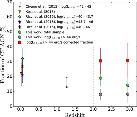
Fraction of CT AGNs in sample obtained from the COSMOS survey (in green) compared with the CT fraction obtained by Koss et al. (2016) from the BAT catalogue (orange), to the CT fraction found by Ricci et al. (2015) in the nearby Universe and to the fraction obtained by Civano et al. (2015) in the redshift range z = 0.04–2.5 (dark grey). Using simulations, we calculated the fraction of CT AGNs that we are not able to detect due to Chandra flux limit. The fraction of CT AGNs from the COSMOS catalogue corrected for the fraction of CT AGNs we are not able to detect (in red) shows a constant behaviour.
5 SUMMARY AND CONCLUSIONS
We extended the SC method, developed by Koss et al. (2016), to Chandra observations at redshifts between 2 and 5. We summarize in the following our main findings:
The SC method can be applied to high-redshift AGN observations. The redshift dependence can be corrected by adding a redshift parameter in the SC equation. The method successfully selects simulated CT sources from merely obscured ones.
We applied the SC method to the CDF-S survey. The SC method selects three sources as CT candidates. One of these is the proposed CT AGNs from Gilli et al. (2011) at redshift z = 4.67. The fraction of CT AGNs we selected from the sources with spectroscopic redshift is 17|$^{+19}_{-11}\hbox{\,per\,cent}$|.
We applied the method also to the COSMOS-legacy survey, constraining our analysis to sources at redshifts between 2 and 5 with more than 10 counts. In total, the method selected 40 from 272 sources as CT candidates (14.5 per cent). After correcting for biases due to the redshift and accounting for the faint sources that Chandra is not able to detect, we obtain a CT fraction of ∼32 ± 10 per cent, which is a value similar to the one found in Buchner et al. (2015).
We find that the fraction of CT AGNs does not show redshift evolution, which is comparable to the result found by Buchner et al. (2015) in the luminosity range |$\mathrm{{\rm {\it L}}_{2{\rm -}10keV}=10^{43.2{\rm -}46}\, erg\, s^{-1}}$|. However, the fraction that we obtain is similar to the one found by Ricci et al. (2015) in the nearby Universe and by Civano et al. (2015) at redshift z = 0.04–2.5 and much lower than the one obtained by Buchner et al. (2015). This could be explained by the larger luminosity range analysed in Buchner et al. (2015).
Our measured CT fraction from COSMOS is somewhat higher though in agreement within error of the value of 22 per cent found by Koss et al. (2016). The mean luminosity of our sample is ∼1044 erg s−1, while the mean luminosity of the BAT sources at redshift z < 0.03 is ∼5 × 1042 erg s−1. The fraction that we obtain is similar to what has been found by Ricci et al. (2015) in the lowest luminosity bin log(L14-195) = 40.0–43.7 erg s−1.
Moreover, the SC method is insensitive to CT AGNs of very higher column densities, e.g. 1025 − 26 cm−2, which would not be detected in the X-rays. This means that we have to treat the obtained CT fraction as a lower limit. Indeed, the obtained fraction of CT sources is lower than predicted by the models from Gilli et al. (2007) and Treister et al. (2009). Another issue is that the accretion rates of CT AGNs may be much higher than their less obscured counterparts (e.g. Koss et al. 2016) and thus even a small fraction may be important for overall black hole growth.
As a further step, the SC method could be extended to other data samples. For example, the serendipitous Chandra Multiwavelength Project (ChaMP) contains a number of promising high-redshift quasars that could satisfy the requirement needed to apply the method. In the coming months, Chandra will perform an observation of the CDF-S totaling 3 Ms that will complete the present survey. The deeper exposures in the 7-Ms catalogue will allow tighter constraints on the fraction of CT AGNs at highredshift.
Acknowledgements
MK acknowledges support from the SNSF through the Ambizione fellowship grant PZ00P2_154799/1. MK and KS acknowledge support from Swiss National Science Foundation Grants PP00P2_138979 and PP00P2_166159. The scientific results reported in this article are based on data obtained from the Chandra Data Archive.
This research made use of Astropy, a community-developed core python package for Astronomy (Astropy Collaboration, 2013) and the NASA's Astrophysics Data System.
The event file can be found on the CXC homepage (http://cxc.harvard.edu/cda/Contrib/CDFS.html)
REFERENCES
SUPPORTING INFORMATION
Supplementary data are available at MNRAS online.
Table 2: SC values for the analysed sample in the COSMOS legacy survey.
Please note: Oxford University Press is not responsible for the content or functionality of any supporting materials supplied by the authors. Any queries (other than missing material) should be directed to the corresponding author for the article.
