


Abstract
We present the second release of value-added catalogues of the LAMOST Spectroscopic Survey of the Galactic Anticentre (LSS-GAC DR2). The catalogues present values of radial velocity Vr, atmospheric parameters – effective temperature Teff, surface gravity log g, metallicity [Fe/H], α-element to iron (metal) abundance ratio [α/Fe] ([α/M]), elemental abundances [C/H] and [N/H] and absolute magnitudes MV and |$M_{K_{\rm s}}$| deduced from 1.8 million spectra of 1.4 million unique stars targeted by the LSS-GAC since 2011 September until 2014 June. The catalogues also give values of interstellar reddening, distance and orbital parameters determined with a variety of techniques, as well as proper motions and multiband photometry from the far-UV to the mid-IR collected from the literature and various surveys. Accuracies of radial velocities reach 5 km s−1 for the late-type stars, and those of distance estimates range between 10 and 30 per cent, depending on the spectral signal-to-noise ratios. Precisions of [Fe/H], [C/H] and [N/H] estimates reach 0.1 dex, and those of [α/Fe] and [α/M] reach 0.05 dex. The large number of stars, the contiguous sky coverage, the simple yet non-trivial target selection function and the robust estimates of stellar radial velocities and atmospheric parameters, distances and elemental abundances make the catalogues a valuable data set to study the structure and evolution of the Galaxy, especially the solar-neighbourhood and the outer disc.
1 INTRODUCTION
Better understanding the structure, stellar populations and the chemical and dynamic evolution of the Milky Way is both a challenge and an opportunity of modern galactic astronomy. The Milky Way is the only galaxy whose distribution of stellar populations can be mapped out in full dimensionality – three-dimensional position and velocity, age, as well as photospheric elemental abundances. However, owing to our location inside the Milky Way disc, the hundreds of billions of Galactic stars are distributed over the whole sky, and our views in the Galactic disc are seriously limited by the interstellar dust extinction. Obtaining the full dimensional distribution of a complete stellar sample is thus a great challenge. It is only recently that comprehensive surveys of Galactic stars become feasible, thanks to the implementation of a number of large-scale photometric and spectroscopic surveys, such as the Sloan Digital Sky Survey (SDSS; York et al. 2000), the Two Micron All Sky Survey (2MASS; Skrutskie et al. 2006), the Apache Point Observatory Galactic Evolution Experiment (APOGEE; Majewski et al. 2010), the LAMOST Experiment for Galactic Understanding and Exploration (LEGUE; Deng et al. 2012; Zhao et al. 2012) and the Gaia astrometric survey (Perryman et al. 2001; Gaia Collaboration et al. 2016).
As a major component of the LEGUE project, the LAMOST Spectroscopic Survey of the Galactic Anticentre (LSS-GAC; Liu et al. 2014; Yuan et al. 2015) is being carried out with the aim to obtain a statistically complete stellar spectroscopic sample in a contiguous sky area around the Galactic anticentre, taking full advantage of the large number of fibers (4000) and field of view (20 deg2) offered by LAMOST (Cui et al. 2012). The survey will allow us to acquire a deeper and more comprehensive understanding of the structure, origin and evolution of the Galactic disc and halo, as well as the transition region between them. The main scientific goals of LSS-GAC include: (1) to characterize the stellar populations, chemical composition, kinematics and structure of the thin and thick discs and their interface with the halo, (2) to understand the temporal and secular evolution of the disc(s), (3) to probe the gravitational potential and dark matter distribution, (4) to identify star aggregates and substructures in the multidimensional phase space, (5) to map the interstellar extinction as a function of distance, (6) to search for and study rare objects (e.g. stars of peculiar chemical composition or hypervelocities) and (7) to study variable stars and binaries with multi-epoch spectroscopy.
LSS-GAC plans to collect low-resolution (R ∼ 1800) optical spectra (λλ3700–9000 Å) of more than 3 million stars down to a limiting magnitude of r ∼ 17.8 mag (to 18.5 mag for selected fields) in a contiguous sky area of over 3400 deg2 centred on the Galactic anticentre (|b| ≤ 30°, 150° ≤ l ≤ 210°), and deliver spectral classifications, stellar parameters (radial velocity Vr, effective temperature Teff, surface gravity log g, metallicity [Fe/H], α-element to iron abundance ratio [α/Fe] and individual elemental abundances), as well as values of interstellar extinction and distance of the surveyed stars, so as to build up an unprecedented, statistically representative multidimensional data base for the Galactic (disc) studies. The targets of LSS-GAC are selected uniformly in the planes of (g − r, r) and (r − i, r) Hess diagrams and in the (RA, Dec.) space with a Monte Carlo method, based on the Xuyi Schmidt Telescope Photometric Survey of the Galactic Anticentre (XSTPS-GAC; Zhang et al. 2013, 2014; Liu et al. 2014; Yuan et al. 2015), a CCD imaging photometric survey of ∼7000 deg2 with the Xuyi 1.04-/1.20-m Schmidt Telescope. Stars of all colours are sampled by LSS-GAC. The sampling rates are higher for stars of rare colours, without losing the representation of bulk stars, given the high sampling density (≳1000 stars per deg2). This simple yet non-trivial target selection strategy allows for a statistically meaningful study of the underlying stellar populations for a wide range of object class, from white dwarfs (e.g. Rebassa-Mansergas et al. 2015), main-sequence turn-off stars (e.g. Xiang et al. 2015a) to red clump giants (e.g. Huang et al. 2015a), after the selection function has been properly taken into account.
As an extension, LSS-GAC also surveys objects in a contiguous area of a few hundred deg2 around M31 and M33. The targets include background quasars, planetary nebulae (PNe), H ii regions, globular clusters, supergiant stars, as well as foreground Galactic stars. In addition, to make full use of all available observing time, LSS-GAC targets very bright (VB) stars of r < 14 mag in sky areas accessible to LAMOST (−10° ≤ Dec. ≤ 60°) in poor observing conditions (bright/grey lunar nights, or nights of poor transparency). Those VB stars comprise an excellent sample supplementary to the main one. Given their relatively low surface densities, at least for the areas outside the disc, LSS-GAC has achieved a very high sampling completeness (50 per cent) for those VB stars, making the sample a gold mine to study the solar-neighbourhood.
Radial velocities and atmospheric parameters (effective temperature Teff, surface gravity log g, metallicity [Fe/H]) have been deduced from the LSS-GAC spectra for A/F/G/K-type stars using both the official LAMOST Stellar parameter Pipeline (LASP; Wu et al. 2011, 2014) and the LAMOST Stellar Parameter Pipeline at Peking University (LSP3; Xiang et al. 2015b). Typical precisions of the results, depending on the spectral signal-to-noise ratio (SNR) and the spectral type, are a few km s−1 for radial velocity Vr, 100–200 K for Teff, 0.1–0.3 dex for log g, 0.1–0.2 dex for [Fe/H] (Gao et al. 2015; Luo et al. 2015; Xiang et al. 2015b; Ren et al. 2016; Wang et al. 2016b). Values of α-element to iron abundance ratio [α/Fe], as well as abundances of individual elements (e.g. [C/H] and [N/H]), have also been derived with LSP3 (Li et al. 2016; Xiang et al. 2017), with precisions similar to those achieved by the APOGEE survey for giant stars (Xiang et al. 2017). Efforts have also been made to derive stellar parameters from LAMOST spectra with other pipelines, such as the SEGUE Stellar Parameter Pipeline (SSPP; Lee et al. 2015) and the Cannon (Ho et al. 2016). Liu et al. (2015) estimate log g using a support vector regression model based on Kepler asteroseismic measurements of giant stars. Stellar extinction and distances have been deduced for LSS-GAC sample stars using a variety of methods (Chen et al. 2014; Carlin et al. 2015; Yuan et al. 2015; Wang et al. 2016a), with typical uncertainties of EB − V of about 0.04 mag, and of distance between 10 and 30 per cent, depending on the stellar spectral type (Yuan et al. 2015).
Following a year-long Pilot Survey, LSS-GAC was initiated in 2012 October, and is expected to be complete in the summer of 2017. The LSS-GAC data collected up to the end of the first year of the Regular Survey are public available from two formal official data releases, namely the early (LAMOST EDR; Luo et al. 2012) and first (LAMOST DR1; Luo et al. 2015) data release.1 The LAMOST EDR includes spectra and stellar parameters derived with the LASP for stars observed during the Pilot Survey, while the LAMOST DR1 includes stars observed by 2013 June. In addition, there is a public release of LSS-GAC value-added catalogues for stars observed by 2013 June, i.e. the LSS-GAC DR12 (Yuan et al. 2015). LSS-GAC DR1 presents stellar parameters derived with LSP3, values of interstellar extinction and stellar distance deduced with a variety of methods, as well as magnitudes of broad-band photometry compiled from various photometric catalogues [(e.g. Galaxy Evolution Explorer (GALEX), SDSS, XSTPS-GAC, UCAC4, 2MASS and Wide-field Infrared Survey Explorer (WISE)], and values of proper motions from the UCAC4 and PPMXL catalogues and those derived by combing the XSTPS-GAC and 2MASS astrometric measurements, and, finally, stellar orbital parameters (e.g. eccentricity) computed assuming specific Galactic potentials.
This paper presents the second release of value-added catalogues of LSS-GAC (LSS-GAC DR2). LSS-GAC DR2 presents the aforementioned multidimensional parameters deduced from 1796 819 spectra of 1408 737 unique stars observed by 2014 June. Compared to LSS-GAC DR1, in addition to a significant increase in stellar number, several improvements to the data reduction and stellar parameter determinations have been implemented, including: (1) an upgraded LAMOST two-dimensional pipeline has been used to process the spectra; (2) the spectral template library used by LSP3 has been updated, adding more than 200 new templates. The atmospheric parameters for all template stars have also been re-determined/calibrated; (3) values of α-element to iron abundance ratio [α/Fe] have been estimated with LSP3; (4) accurate values of stellar atmospheric parameters (Teff, log g, [Fe/H], [α/Fe]), absolute magnitudes MV and |$M_{K_{\rm s}}$|, as well as elemental abundances [C/H] and [N/H], have also been estimated from the spectra using a multivariate regression method based on kernel-based principal component analysis (KPCA).
The paper is organized as follows. Section 2 describes the observations of LSS-GAC DR2, including a brief review of the target selection algorithm and the observational footprint. Section 3 introduces the data reduction briefly. Section 4 presents a detailed description of the improvements in stellar parameter determinations incorporated in LSS-GAC DR2. Section 5 briefly discusses the duplicate observations, which accounts for nearly 30 per cent of all observations. Section 6 introduces the determinations of extinction and distance. Section 7 presents the proper motions and derivation of stellar orbital parameters. The format of value-added catalogues is described in Section 8, followed by a summary in Section 9.
2 OBSERVATIONS
To make good use of observing time of different qualities as well as to avoid fibre cross-talking, LSS-GAC stars are targeted by four types of survey plates defined based on r-band magnitude (Liu et al. 2014; Yuan et al. 2015). Stars of r < 14.0 mag are targeted by the VB plates, and observed in grey/lunar nights, with typical exposure time of (2–3) × 600 s. Stars of 14.0 < r ≲ 16.3 mag are targeted by bright (B) plates, and observed in grey/dark nights, with a typical exposure time of 2 × 1200 s, whereas stars of 16.3 ≲ r ≲ 17.8 mag, and of 17.8 ≲ r < 18.5 mag are targeted, respectively, by medium-bright (M) and faint (F) plates, and observed in dark nights of excellent observing conditions (in term of seeing and transparency), with a typical exposure time of 3 × 1800 s.
By 2014 June, 314 plates (194 B + 103 M + 17 F) for the LSS-GAC main survey, 59 plates (38 B + 17 M + 4 F) for the M31/M33 survey and 682 plates for the VB survey have been observed. Note that the spectra of a few plates could not be successfully processed with the two-dimensional pipeline and are therefore not included in the above statistics. During the survey, some observing time, on the level of one or two grey nights per month, has been reserved for monitoring the instrument performance (e.g. throughput and accuracy of fibre positioning; Liu et al. 2014; Yuan et al. 2015). Some of those reserved nights have been used to target some of the LSS-GAC plates, yielding another 94 observed plates (79 B/M/F + 15 V). Finally, 43 B or M or F LSS-GAC plates were observed from 2011 September to October, when the LAMOST was being commissioned before the start of Pilot Survey. For those 43 plates, the magnitude limits of assigning stars in B/M/F plates are not exactly the same as those adopted during the Pilot and Formal surveys. For convenience, all plates observed using reserved time as well as those collected during the commissioning phase have been grouped into, as appropriately, the LSS-GAC main, M31/M33 and VB survey, respectively, leading to a total of 395 plates for the LSS-GAC main, 100 plates for the M31/M33 and 697 plates of the VB survey, respectively.
The total numbers of spectra collected and unique stars targeted by those plates are listed in Table 1. Table 1 also lists the numbers of spectra and unique stars that are successfully observed, defined by a spectral SNR of higher than 10 either in the blue (∼4650 Å) or the (∼7450 Å) part of the spectrum (Liu et al. 2014). The numbers of spectra and stars have increased significantly compared to those of LSS-GAC DR1 that contains, for example, 225 522 spectra of 189 042 unique stars of SNR(4650 Å) >10 for the main survey, and 457 906 spectra of 385 672 unique stars of SNR(4650 Å) >10 for the VB survey (cf. Yuan et al. 2015). Due to the overlapping of LAMOST fields of view of adjacent plates, and the repeating of observations failing to meet the quality control, there is a considerable fraction of stars that have been repeatedly targeted several times. For LSS-GAC DR2, amongst the 948 361 unique stars targeted by the main survey, 71.0, 20.6, 6.0, 1.7, 0.5 and 0.1 per cent of the stars are observed by one to six times, respectively. The corresponding fractions for the M31/M33 survey are 60.1, 20.4, 10.1, 4.4, 2.5 and 1.3 per cent, and those for the VB survey are 73.5, 20.5, 3.7, 1.7, 0.3 and 0.2 per cent. For those unique stars with SNR(4650 Å) >10, the corresponding fractions are 83.6, 13.2, 2.4, 0.6, 0.1 and 0.03 per cent for the LSS-GAC main survey, 72.6, 19.2, 5.6, 1.7, 0.7 and 0.2 per cent for the M31/M33 survey, and 78.3, 17.3, 2.9, 1.2, 0.2 and 0.1 per cent for the VB survey. Note that there are also a small fraction (∼0.8 per cent) of stars that are targeted by both the LSS-GAC main (or M31/M33) survey and the VB survey. These duplicates were not considered when calculating the above percentage numbers.
Numbers of spectra and unique stars (in parentheses) observed by LSS-GAC till 2014 June.
| LSS-GAC main survey | M31/M33 survey | VB survey | |
| All SNRs | 1332 812 (948 361) | 305 226 (171 259) | 1944 525 (1431 219) |
| SNR (4650 Å) >10 | 510 531 (423 503) | 91 921 (65 841) | 1194 367 (922 935) |
| SNR (7450 Å) >10 | 688 459 (572 438) | 68 380 (58 197) | 1358 618 (1050 143) |
| SNR (4650 Å) >10 or SNR(7450) >10 | 763 723 (618 924) | 113 597 (80 452) | 1397 538 (1075 677) |
Fig. 1 plots the footprints of the main and M31/M33 surveys, while Fig. 2 plots the footprints of the VB survey. For the main survey, the strategy is to extend the observations of a stripe of Dec. ∼29° to both higher and lower declinations (Yuan et al. 2015). Compared to LSS-GAC DR1, LSS-GAC DR2 has completed two more stripes for B and M plates, namely those of Dec. ∼34° and ∼24°, respectively. A few B and M plates of Galactic latitude b > 35° were observed using either the reserved time or during the commissioning phase. For the M31/M33 survey, seven B and nine M plates were collected in the second year of the Regular Survey (2013 September–2014 June), leading to a much larger sky coverage compared to LSS-GAC DR1. Significant progress in the observation of VB plates is seen in LSS-GAC DR2, in term of both the area and continuity of the sky coverage.
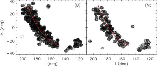
LSS-GAC DR2 footprints in a Galactic coordinate system of stars observed, respectively, with bright (B; left-hand panel) and medium (M; right-hand panel) plates. The red line denotes a constant declination of 30°. To reduce the figure file size, only 1 in 10 observed stars is plotted.
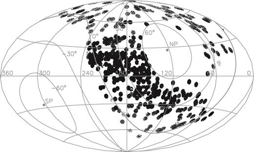
LSS-GAC DR2 footprint for the VB plates. To reduce the figure file size, only 1 in 10 observed stars is plotted.
Figs 3– 5 plot the density distributions of stars targeted, as well as those successfully observed (i.e. with a spectral SNR higher than 10, either in the blue or red), in the colour–magnitude diagrams (CMDs) for the main, M31/M33 and VB surveys, respectively. For the main and M31/M33 surveys, the diagrams are for colour–magnitude combinations (g − r, r) and (r − i, r) used to select targets (Yuan et al. 2015). Magnitudes of g, r, i bands are from the XSTPS-GAC survey, except for a few plates of high Galactic latitudes, for which magnitudes from the SDSS photometric survey are used. The figures show that, as planned, stars of all colours have been observed. Figs 3– 5 also show that the distributions of stars that have either a blue or red spectral SNR higher than 10, as plotted in the middle panels of those three figures, are quite similar to those targeted, plotted in the top panels of the three figures, except for faint ones (r > 17.8 mag). Note that for the main and M31/M33 surveys, some stars of either r > 18.5 or r < 14.0 mag were observed during the commissioning phase. In contrast, the distributions of stars of SNR(4650 Å ) > 10 are quite different – there are fewer faint stars of red colours. This is caused by a combination of the effects of low intrinsic fluxes in the blue of red stars and the lower throughputs of the spectrographs in the blue compared to those in the red (Cui et al. 2012). For the VB survey, (g − r, r) and (J − Ks, J) diagrams are plotted. The g, r, i magnitudes are taken from the AAVSO Photometric All-Sky Survey (APASS; Munari et al. 2014), which have a bright limiting magnitude of about 10 mag and a faint limiting magnitude (10σ) of about 16.5 mag in g, r, i bands. For stars of r > 14.0 mag, magnitudes from the XSTPS-GAC or SDSS surveys are adopted if available. A comparison of stars common to XSTPS-GAC and APASS surveys shows good agreement in both magnitudes and colours for stars of 14.0 < r < 15.0 mag, with differences of just a few (<5) per cent. Due to the heterogeneous input catalogues and magnitude cut criteria used for the VB survey (Yuan et al. 2015), the morphologies of CMD distributions of VB plates are more complicated than those of the main and M31/M33 plates. Nevertheless, due to the high sampling rates of the VB stars (e.g. Xiang et al. 2015a), and the fact that stars of all colours have been observed without a strong colour bias, the selection function can still be well accounted for with some effort and care, if not straightforward. Fig. 6 plots the SNR distribution of spectra for the main, M31/M33 and VB surveys, as well as those of the whole sample for dwarf and giant stars. Only spectra with either SNR (4650 Å) or SNR (7450 Å) higher than 10 are plotted. The number of spectra in logarithmic scale decreases approximately linearly with increasing SNR. SNRs of the red part of the spectra are generally higher than those of the blue part. Also, spectra of the VB survey have generally higher SNRs than those of the main and M31/M33 surveys. Distribution of SNRs for the giants are similar to those of the dwarfs. Here the classification of dwarfs and giants is based on the results of LSP3 (cf. Section 4). For the whole sample, about 36, 57 and 73 per cent of the spectra have an SNR higher than 50, 30 and 20, respectively, in the blue part of the spectrum.
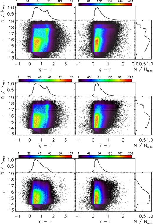
Colour-coded stellar density distributions in the colour–magnitude (g − r, r) and (r − i, r) diagrams for the LSS-GAC main survey. The upper panels show all observed stars, while the middle panels show those with either SNR(4650 Å) > 10 or SNR(7450 Å) > 10, and the lower panels show those with SNR(4650 Å) >10. The histograms show the one-dimensional distributions of stars in colours (g − r) and (r − i) or in magnitude r, respectively, normalized to the maximum value.
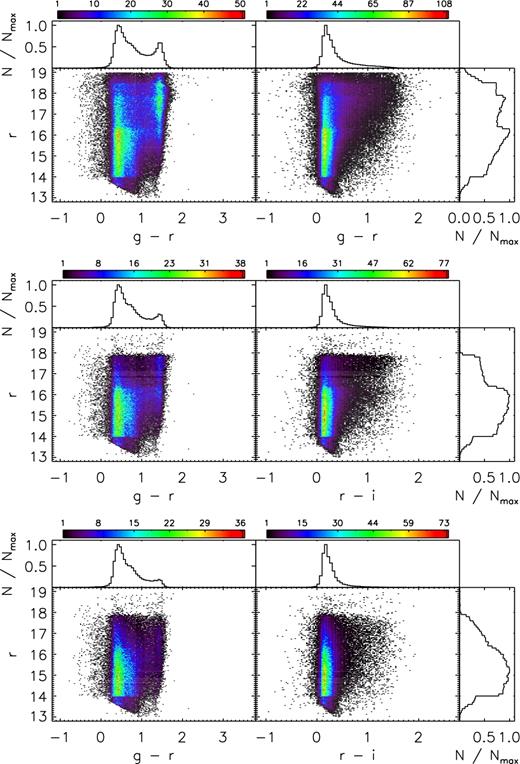
Same as Fig. 3 but for the M31/M33 survey.
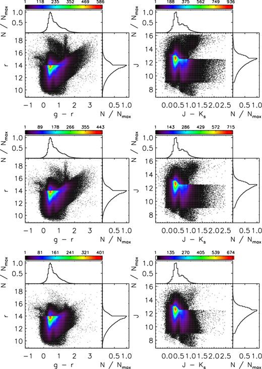
Same as Fig. 3 but for the VB survey. CMDs of (g − r, r) and (J − Ks, J) are shown.
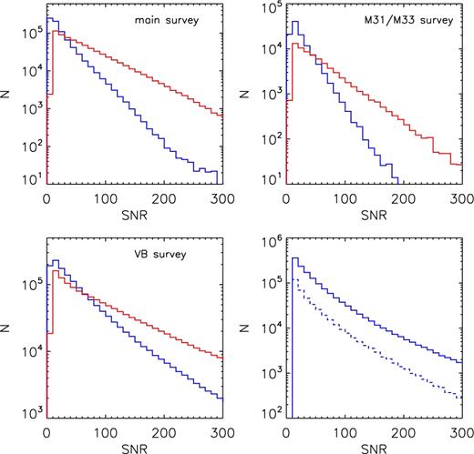
Distribution of spectral SNRs for the main (top left-hand panel), M31/M33 (top right-hand panel) and VB (bottom left-hand panel) surveys. Blue and red lines represent spectral SNR at 4650 and 7450 Å, respectively. The bottom right-hand panel plots SNR (4650 Å) for the whole sample that have a spectral SNR (4650 Å) higher than 10 for dwarfs (solid line) and giants (dashed line), respectively.
3 DATA REDUCTION
The raw spectra of LSS-GAC used to generate the value-added catalogues were processed at Peking University with the LAMOST two-dimensional reduction pipeline (Luo et al. 2012, 2015) to extract the one-dimensional spectra. This process includes several basic reduction steps, including bias subtraction, fibre tracing, fibre flat-fielding, wavelength calibration and sky subtraction. Both fibre tracing and flat-fielding were first carried out using twilight flat-fields. The results were further revised using sky emission lines when processing the object spectra to account for the potential shifts of fibre traces and the variations in fibre throughput. Typical precision of fibre flat-fielding, as indicated by the dispersions of flat-fields acquired in different days, is better than 1 per cent. Wavelength calibration was carried out using exposures of a Cd–Hg arc lamp for the blue-arm spectra and an Ar–Ne arc lamp for the red-arm spectra. Typically, the residuals of wavelength calibration for the individual arc lines have a mean value close to zero and a standard deviation of ∼0.02 Å, which corresponds to ∼1 km s−1 in velocity space. When processing the object spectra, sky emission lines are used to adjust the wavelengths to account for any residual systematic errors in the wavelength calibration and/or potential wavelength drifts between the arc-lamp and object spectra. A comparison of stellar radial velocities with the APOGEE measurements for LAMOST-APOGEE common stars yields an offset of −3 to −4 km s−1 (Luo et al. 2015; Xiang et al. 2015b), and the offset is found to be stable in the past few years, with typical night-to-night variations of about 2 km s−1. For each of the 16 spectrographs, about 20 fibres are typically assigned to target sky background for sky subtraction. The numbers of sky fibres allocated for sky measurement are higher for plates of low source surface density, e.g. VB plates of |b| > 10°. To subtract the sky background, the two-dimensional pipeline creates a supersky by the B-spline fitting of fluxes measured by the individual sky fibres. The measured fluxes of sky emission lines in the object spectra are normalized to those of the super-sky spectrum to correct for potential differences of throughputs of fibres used to measure the sky and the objects. The correction assumes that the strengths of the sky emission lines are constant across the sky area covered by a given spectrograph, which is about 1 deg2, and any differences in sky emission-line fluxes, as measured by the sky and object fibres, are caused by errors in flat-fielding. The correction also assumes that for the sky background, the continuum scales with emission-line flux.
The resultant one-dimensional spectra were then processed with the flux calibration pipeline developed specifically for LSS-GAC to deal with fields of low Galactic latitudes that may suffer from substantial interstellar extinction. The pipeline generates flux-calibrated spectra as well as co-adds the individual exposures of a given plate (Xiang et al. 2015c; Yuan et al. 2015). To deal with the interstellar extinction, the pipeline calibrates the spectra in an iterative way, using F-type stars selected based on the stellar atmospheric parameters yielded by LSP3 as flux standards. The theoretical synthetic spectra from Munari et al. (2005) of the same atmospheric parameters are adopted as the intrinsic spectral energy distributions (SEDs) of the standards. Typical (relative) uncertainties of the spectral response curves thus derived are about 10 per cent for the wavelength range of 4000–9000 Å (Xiang et al. 2015c).
Compared to the pipelines used to generate LSS-GAC DR1, a few improvements have been implemented: (1) Several fibres of Spectrograph #4 are found to be misidentified before 2013 June (Luo, private communication). As a result, the coordinates, magnitudes, spectra and stellar parameters of stars targeted by those fibres were wrongly assigned in LAMOST DR1 (Luo et al. 2015) as well as LSS-GAC DR1 (Yuan et al. 2015). The fibres are: #76 (87), 87 (79), 79 (95), 95 (84), 84 (76), 44 (31), 31 (46), 46 (26) and 26 (44), where the numbers in the brackets are the correct ones. The errors have been corrected; (2) The values of interstellar reddening of flux standard stars are now derived with the star-pair method (Yuan et al. 2015), replacing those deduced by comparing the observed and synthetic colours, as adopted in LSS-GAC DR1. The change is based on the consideration that the star-pair method for extinction determination is model-free, and yields, in general, more robust results than the method adopted for LSS-GAC DR1 (Yuan et al. 2015); (3) For the flux calibration of VB plates, g, r, i magnitudes from the APASS survey (Munari et al. 2014) are combined with 2MASS J, H, Ks magnitudes to derive values of extinction of flux calibration standard stars. In LSS-GAC DR1, only 2MASS J, H, Ks magnitudes were used. The change should significantly improve the accuracy of extinction estimates for standards used to flux-calibrate VB plates.
Considering that the SNR alone does not give a fully description of the quality of a spectrum, a few flags are now added to the image header of a processed spectrum. The first flag is the ratio of (sky-subtracted) stellar flux to the flux of (super-) sky adopted for sky-subtraction. Due to the uncertainties in sky-subtraction, the spectra of some stars, especially those observed under bright lunar conditions, may have artificially high SNRs, yet this ratio can be, in fact, quite small for those spectra. The flag is denoted by ‘OBJECT_SKY_RATIO’ in the value-added catalogues. A second flag is used to mark fibres that maybe potentially affected by the nearby saturated fibres. Saturation occurs for the VB stars. When a fibre saturates, spectra of nearby fibres, especially those of faint stars, can be seriously contaminated by flux crosstalk, leading to incorrect SNRs and wrongly estimated stellar parameters. When a fibre saturates, stars observed by the adjacent 50 fibers (±25) are now marked by flag ‘SATFLAG’ in the value-added catalogues. Even when a fibre is not saturated, crosstalk may still occur if the flux of that fibre is very high. To account for such situation, a third flag is introduced. If the spectrum from a given fibre has an SNR higher than 300, then the adjacent 4 (±2) fibres are assigned a ‘BRIGHTFLAG’ value of 1; otherwise, the flag has a value of 0. For each fibre, the value of maximum SNR of the nearest five fibres (the adjacent four plus the fibre of concern itself) is also listed as ‘BRIGHTSNR’ in the value-added catalogues. Finally, a flag has been created to mark bad fibres. Among the 4000 fibres of LAMOST, some have very low throughputs or suffer from serious positioning errors. Spectra yielded by those ‘bad’ fibers cannot be trusted. The number of bad fibres continuously increases with time, and reaches about 200 by 2014 June. Those fibers are marked by ‘BADFIBRE’ in the value-added catalogues. In addition to those newly created flags, information of observing conditions with regard to the moon (phase, angular distance), the airmass and the pointing position of the telescope are now also included in LSS-GAC DR2.
4 STELLAR PARAMETER DETERMINATION: IMPROVEMENTS OF LSP3
LSS-GAC DR1 presents values of radial velocity Vr and stellar atmospheric parameters (effective temperature Teff, surface gravity log g, metallicity [Fe/H]) derived from LSS-GAC spectra with LSP3. Since then, a few improvements of LSP3 have been implemented and are included in LSS-GAC DR2, including: (1) A number of new spectral templates have been added to the MILES library, and atmospheric parameters of the template stars have been re-determined/calibrated; (2) Several flags are now assigned to describe the best-matching templates that have the characteristics of a, for example, variable star, binary, double/multiple star or supergiant, etc., of a given target spectrum; (3) Values of α-element to iron abundance ratio [α/Fe] have been estimated by template matching with a synthetic spectral library; (4) A multivariate regression method based on KPCA has been used to obtain an independent set of estimates of stellar atmospheric parameters, including Teff, log g, [M/H], [Fe/H], [α/M], [α/Fe], absolute magnitudes MV and |$M_{K_{\rm s}}$| as well as individual elemental abundances including [C/H] and [N/H].
4.1 Updates to the MILES library
The original MILES spectral library contains medium-to-low resolution (full width at half-maximum, FWHM ∼2.5 Å) long-slit spectra of the wavelength range of 3525–7410 Å for 985 stars that have robust stellar parameter estimates in the literature, mostly determined with high-resolution spectroscopy (Sánchez-Blázquez et al. 2006; Falcón-Barroso et al. 2011). The MILES library is adopted by LSP3 as templates for estimation of atmospheric parameters from LAMOST spectra. Compared to other template libraries available in the literature, MILES has two advantages. First, the MILES spectra have robust flux calibration and the spectral resolution matches well that of the LAMOST spectra. Secondly, the template stars cover a large volume of parameter space (3000 < Teff < 40, 000 K, 0 < log g < 5 dex and −3.0 < [Fe/H] < 0.5 dex).
Still, for the purpose of accurate stellar atmospheric parameter estimation, the MILES library has a few defects in need of improvement. One is the limited spectral wavelength coverage. LAMOST spectra cover the full optical wavelength range of 3700–9000 Å, whereas MILES spectra stop at 7410 Å in the red. As a result, LAMOST spectra in the 7400–9000 Å wavelength range have hitherto not been utilized for parameter estimation. There are a few prominent features in this wavelength range that are sensitive abundance indicators, including, e.g. the Ca ii λλ8498, 8542, 8664 triplet and the Na i λλ8193, 8197 doublet. In addition, since LSS-GAC targets stars of all colours, especially those in the disc, about 30 per cent spectra collected have poor SNRs in the blue but good SNRs in the red. Those stars are either intrinsically red or suffer from heavy interstellar extinction. Stellar parameters for those stars have currently not been derived from LAMOST spectra, by either LSP3 or LASP, due to the fact that both the MILES and ELODIE (adopted by LASP) libraries do not have wavelength coverage long enough in the red. Another defect of the MILES library is the inhomogeneous coverage of stars in the parameter space. As shown in Xiang et al. (2015b), there are holes and clusters in the distribution of MILES stars in the parameter space, leading to some significant artefacts in the resultant parameters. Finally, stellar atmospheric parameters of the original MILES library are collected from various sources in the literature, which thus suffer from systematic errors. Although Cenarro et al. (2007) have taken the effort to homogenize the parameters in order to account for the systematics amongst the values from the different sources, the homogenization was carried out for only a limited temperature range of 4000 < Teff < 6300 K. With more data available, there is a room for considerable improvement.
To deal with the limited wavelength coverage of the MILES spectra and to improve the coverage and distribution of template stars in the parameter space, an observational campaign is being carried out to observe additional template stars that fill the holes in parameter space, to enlarge the coverage of parameter space, as well as to extend the spectral wavelength coverage to 9200 Å, using the NAOC 2.16-m telescope and the YAO 2.4-m telescope (Wang et al., in preparation). The project plans to obtain long-slit spectra covering 3600–9200 Å for some 900 template stars newly selected from the PASTEL catalogue (Soubiran et al. 2010), which is a compilation of stars with robust stellar parameters, mostly inferred from high-resolution spectroscopy. The project will also extend the wavelength coverage of all the original MILES spectra to 9200 Å. In this work, 267 new template spectra obtained by the campaign till 2015 October have been added to the MILES library to generate parameter estimates presented in LSS-GAC DR2. In addition, to reduce systematic and random errors of the atmospheric parameters of the template stars, Huang et al. (in preparation) have re-calibrated/determined the atmospheric parameters of all template stars, both old and newly selected. In doing so, the recent determinations of parameters of template stars available from the PASTEL catalogues have been adopted, replacing the older values used by the original MILES library. The updated values of metallicity are then used to calculate effective temperatures using the newly published metallicity-dependent colour–temperature relations of Huang et al. (2015c), deduced from more than two hundred nearby stars with direct, interferometric angular size measurements and Hipparcos parallaxes. Values of surface gravity are re-determined using Hipparcos parallaxes (Perryman et al. 1997; Anderson & Francis 2012) and stellar isochrones from the Dartmouth Stellar Evolution Database (Dotter et al. 2008). Values of [Fe/H] are then re-calibrated to the standard scale of Gaia-ESO survey (Jofré et al. 2015). Fig. 7 plots the newly calibrated/determined parameters of the template stars in the Teff–log g and Teff–[Fe/H] planes. Note that in generating LSS-GAC DR1, 85 of the original MILES stars were abandoned because there were no complete parameter estimates in the literatures. Those stars are now included in the library as their parameters have been re-determined. Also, with the newly selected and observed templates added to the library, we have now discarded the 400 interpolated spectra used when generating LSS-GAC DR1.
![Distributions of template stars used by LSP3 in the Teff–log g and Teff–[Fe/H] planes. Black dots represent stars in the original MILES library, while red dots represent 267 newly observed templates employed in the generation of LSS-GAC DR2 (see the text).](https://oup.silverchair-cdn.com/oup/backfile/Content_public/Journal/mnras/467/2/10.1093_mnras_stx129/3/m_stx129fig7.jpeg?Expires=1750294842&Signature=TdgtrRWPZhzJQezgAKGoFhxr1A7PrtQythW5uD9B-vr5kQQlguTEUIFdyruuPb7LABlEohbOEKJAtdQKRUsx2TsZDo27CUcar3-qdSCKcFnyWLKNCeb28aoiGiOu49hh7EHHgPlb1M0zwkvbE6wCvoNmgr0EZqMFl5ysQSBthVgz2XSwr25M0aIZqbBUd1PElNKKjgBhQMSfe4dCFAJo7IpruJsHoQa64ZYKvecEpbjokPRlnBj5ZQEmURT74HY0BW2Aso0g8~9Ll8Y~UR7OqofEmN1Xr3F5erua0jQ3aN39ZsSG4lqlPvRV6XglLNX~yQg-I6T0~tzmLMeUxk2EuQ__&Key-Pair-Id=APKAIE5G5CRDK6RD3PGA)
Distributions of template stars used by LSP3 in the Teff–log g and Teff–[Fe/H] planes. Black dots represent stars in the original MILES library, while red dots represent 267 newly observed templates employed in the generation of LSS-GAC DR2 (see the text).
4.2 [α/Fe] estimation by matching with synthetic spectra
α-element to iron abundance ratio [α/Fe] is a good indicator of the Galactic chemical enrichment history (e.g. Lee et al. 2011), and thus valuable to derive. To estimate [α/Fe] from LAMOST spectra, a method of template matching based on χ2-fitting with synthetic spectra is developed for LSP3. Details about the method and robustness tests of the deduced [α/Fe] values are described in Li et al. (2016). Here we briefly summarize the method and point out a few improvements that may lead to better results.
The synthetic library used to estimate [α/Fe] was generated with the spectrum code (Gray 1999) of version 2.76, utilizing the Kurucz stellar model atmospheres of Castelli & Kurucz (2004). The solar [α/Fe] ratio is set to zero, and the α-enhanced grids are generated by scaling the elemental abundances of O, Mg, Si, S, Ca and Ti, and those of C and N abundances are also enhanced by the amount of α-elements. Lines from more than 15 diatomic molecule species, including H2, CH, NH, OH, MgH, AlH, SiH, CaH, C2, CN, CO, AlO, SiO, TiO and ZrO, are taken into account in the calculation of the opacity. Isotope lines are also taken into account. In total, 320 000 synthetic spectra are generated. Table 2 lists the parameter ranges and steps of the grids. Note that the grids adopted here have a step of 0.1 dex in [α/Fe], half of the value used in Li et al. (2016). All the computed synthetic spectra have a resolution of 2.5 Å FWHM, and is invariant with wavelength.
Grids of KURUCZ synthetic spectra for [α/Fe] estimation.
| Parameter | Range | Step |
|---|---|---|
| Teff | [4000, 8000] K | 100 K |
| log g | [0.0, 5.0] dex | 0.25 dex |
| [Fe/H] | [−4.0, 0.5] dex | 0.2 dex for [Fe/H] < −1.0 dex |
| 0.1 dex for [Fe/H] > −1.0 dex | ||
| [α/Fe] | [−0.4, 1.0] dex | 0.1 dex |
| Parameter | Range | Step |
|---|---|---|
| Teff | [4000, 8000] K | 100 K |
| log g | [0.0, 5.0] dex | 0.25 dex |
| [Fe/H] | [−4.0, 0.5] dex | 0.2 dex for [Fe/H] < −1.0 dex |
| 0.1 dex for [Fe/H] > −1.0 dex | ||
| [α/Fe] | [−0.4, 1.0] dex | 0.1 dex |
For a target spectrum with atmospheric parameters Teff, log g and [Fe/H] yielded by LSP3, the synthetic spectra are interpolated to generate a set of spectra that have the same atmospheric parameters as the target for all grid values of [α/Fe]. Values of χ2 between the target and the individual interpolated synthetic spectra are then calculated. A Gaussian plus a second-order polynomial is then used to fit the deduced χ2 as a function of [α/Fe]. The value of [α/Fe] that yields minimum χ2 is taken to be the [α/Fe] ratio of the target spectrum. To compute χ2, Li et al. (2016) use spectral segments 4400–4600 and 5000–5300 Å. The 4400–4600 Å segment contains mainly Ti features, while that of 5000–5300 Å contains mainly Mg i features, as well as a few features of Ca, Ti and Si. Note that given the low resolution as well as limited SNRs of LAMOST spectra, Ca, Ti and Si features within those two spectral segments contribute, in fact, only a small fraction of the calculated values of χ2, and are therefore not very useful for the determination of [α/Fe]. In metal-rich stars, the Mg i b features are, in general, prominent enough for a robust determination of [α/Fe]. However, in metal-poor ([Fe/H] < −1.0 dex) stars, the Mg i b lines become less prominent so that the [α/Fe] have larger uncertainties. In this work, in order to improve precision of [α/Fe] estimates, especially for metal-poor stars, we have opted to include the 3910–3980 Å spectral segment that contains the Ca ii HK lines in the calculation of χ2 values. Meanwhile, as an option, we also provide results yielded using the exactly same spectral segments as Li et al. (2016). This is useful considering that the strong Ca ii HK lines in model spectra for metal-rich stars are maybe not accurately synthesized.
The resolution of LAMOST spectra from individual fibers varies from one to another, as well as with wavelength (Xiang et al. 2015b). To account for this in template matching, the synthetic spectra are degraded in resolution to match that of the target spectrum. The latter is derived utilizing the arc spectrum. The deduced resolution as a function of wavelength is further scaled to match the resolution yielded by sky emission lines detected in the target spectrum in order to account for systematic variations of spectral resolution between the arc and target exposures. Typically, for a given spectrograph, fibre-to-fibre variations of spectral resolution amount to 0.3 Å, rising to 0.5–1.0 Å among the different spectrographs. Systematic variations of spectral resolution between the arc and target exposures are found to be typically 0.2 Å.
In addition, in order to allow for possible uncertainties in the input atmospheric parameters Teff, log g and [Fe/H] yielded by LSP3 as well as any possible mismatch between the LSP3 atmospheric parameters and those of the Kurucz stellar model atmospheres, in this work, we have opted not to fix the input values of Teff, log g and [Fe/H] as yielded by LSP3, but allow them to vary in limited ranges around the initial values. The ranges are set to 2σ uncertainties of the parameters concerned, with lower limits of 500 K, 0.5 and 0.5 dex, and upper limits of 1000 K, 1.0 and 1.0 dex for Teff, log g and [Fe/H], respectively. For each grid value of [α/Fe], the synthetic spectrum that has atmospheric parameters Teff, log g and [Fe/H] within the above ranges and fits the target spectrum best (i.e. yielding the smallest χ2) is taken as the choice of synthetic spectrum when fitting and deriving [α/Fe] using the technique described in Li et al. (2016).
Values of [α/Fe] are derived with the above algorithm for all LSS-GAC DR2 stars of a spectral SNR higher than 15. The left-hand panel in the third row of Fig. 9 plots the density distribution of LSS-GAC DR2 dwarf stars in the [Fe/H]–[α/Fe] plane. Here, the [α/Fe] are those derived using spectra including the 3910–3980 Å segments. The figure shows an [α/Fe] plateau for metal-poor ([Fe/H] < −1.0 dex) stars, at a median value about 0.4 dex. For more metal-rich stars, [α/Fe] decreases with increasing [Fe/H], reaching a median value of zero near the solar metallicity, which means that the zero-point offset, i.e. deviations of [α/Fe] values from zero at solar metallicity, is small, which is in contrast to Li et al. (2016) who find a zero-point offset of −0.12 dex. However, we indeed find a zero-point offset of about −0.1 dex for [α/Fe] derived using only the 4400–4600 and 5000–5300 Å segments, which is basically consistent with Li et al. (2016). The offset is found to be mainly contributed by the 4400–4600 Å segment. The causes of this difference are not fully understood yet. We suspect there may be some unrealistic inputs in either the atmosphere model or the atomic and molecular data used to generate the synthetic spectra. Note that here we opt not to introduce any external corrections on the estimated [α/Fe]. Random errors of [α/Fe] induced by spectral noises, as estimated by comparing the results deduced from duplicate observations, are a function of spectral SNR and atmospheric parameters Teff, log g and [Fe/H], and have typical values that decrease from ∼0.1 to ∼0.05 dex as the spectral SNR increases from 20 to a value higher than 50. To provide a realistic error estimate for [α/Fe], the random error induced by spectral noises is combined with the method error, which is assumed to have a constant value of 0.09 dex, estimated by a comparison with high-resolution measurements (cf. Li et al. 2016).
For giant stars, [α/Fe] estimated with the above algorithm exhibits a zero-point offset between 0.1 and 0.2 dex, probably caused by inadequacies of the synthetic spectra for giant stars. In this work, no corrections for those offsets are applied. Note that for giant stars, [α/Fe] values are also estimated with the KPCA regression method using the LAMOST-APOGEE common stars as the training data set (cf. Section 4.3), and the resultant values are presented as the recommended ones (cf. Section 4.6).
4.3 Stellar atmospheric parameters estimated with the KPCA method
The LSP3 version used to generate LSS-GAC DR1 estimates stellar atmospheric parameters Teff, log g and [Fe/H] with a χ2-based weighted-mean algorithm. The algorithm achieves a high precision in the sense that random errors of the deduced parameters induced by spectral noises are well controlled, even for stars of SNRs as low as 10. Nevertheless, parameters estimated with the weighted-mean algorithm suffer from several artefacts. One is the so-called suppression effect – values of the derived log g are narrowed down to an artificially small range. This is partly caused by the fact that χ2 calculated from a LAMOST spectrum with respect to a template spectrum is only moderately sensitive to log g, thus the sets of templates used to calculate the weighted-mean values of log g for the individual target sources often have similar distributions in log g. Another artefact is the so-called boundary effect – parameters of stars with true parameters that pass or are close to the boundary of parameter space covered by the templates are often either underestimated or overestimated systematically by the weighted-mean algorithm. This effect is especially serious for [Fe/H] and log g estimation. Finally, due to the inhomogeneous distribution of templates in the parameter space, moderate clustering effect is also seen in the deduced parameter values.
To overcome the above defects of the weighted-mean algorithm, a regression method based on the KPCA has recently been incorporated into LSP3 (Xiang et al. 2017). The method is implemented in a machine learning scheme. A training data set is first defined to extract non-linear principal components (PCs, and the loading vectors) as well as to build up regression relations between the PCs and the target parameters. Four training data sets are defined for the determination of specific sets of parameters of specific types of stars. They are: (1) the MILES library for the estimation of Teff and [Fe/H] of A/F/G/K stars, and for the estimation of log g of stars that have log g values larger than 3.0 dex, as given by the weighted-mean algorithm. The latter stars are mainly dwarfs and sub-giants; (2) a sample of LAMOST-Hipparcos common stars with accurate parallax (thus, distance and absolute magnitude) measurements for the estimation of absolute magnitudes (MV and |$M_{K_{\rm s}}$|) directly from LAMOST spectra; (3) a sample of LAMOST-Kepler common stars with accurate asteroseismic log g measurements for the estimation of log g of giant stars; and (4) a sample of LAMOST-APOGEE common stars for the estimation of metal abundance [M/H], α-element to iron (metal) abundance ratio [α/Fe] ([α/M]) and of individual elemental abundances including [Fe/H], [C/H] and [N/H] for giant stars. A detailed description of the implementation and test of the method is presented in Xiang et al. (2017). Here we note two updates of the implementation with respect to those of Xiang et al. (2017). One is that a unified number of PCs of 100 is adopted except for the estimation of absolute magnitudes with the LAMOST-Hipparcos training set, for which both 100 and 300 PCs are adopted. Another modification is that additional training stars have been added to the LAMOST-Kepler and LAMOST-APOGEE training sets as a result that more common stars become available as the surveys progress. Both training sets now contain (exactly) 3000 stars.
Compared to the weighted-mean results, log g and [Fe/H] derived with the KPCA regression method using the MILES training set have been found to suffer from less systematics, and thus better for statistical analyses. A comparison with asteroseismic measurements shows that for stars of Teff < 6000 K and [Fe/H] > −1.5 dex, uncertainties of KPCA log g estimates can be as small as 0.1 dex for spectral SNRs higher than 50. The uncertainties increase substantially as the SNR deteriorates, reaching ∼0.2 dex at an SNR of 20 (Xiang et al. 2017). Similarly, comparisons with [Fe/H] determinations from high-resolution spectroscopy show that uncertainties of KPCA [Fe/H] estimates are ∼0.1 dex for good SNRs. For metal-poor ([Fe/H] < −1.5 dex) or hot (Teff > 8000 K) stars, KPCA estimates of both log g and [Fe/H] become less reliable, and should be used with caution. Systematic differences between KPCA and weighted-mean estimates of Teff exist for stars hotter than ∼6500 K, with deviations reach as much as ∼300 K for stars of Teff ∼ 7500 K. More studies are needed to understand the cause of deviations. For the time being, we recommend weighted-mean Teff values as they are estimated in a straightforward way and well validated (Xiang et al. 2015b). However, note that weighted-mean estimates of Teff suffer from clustering effect so that they may weakly clump in the parameter space on the scale of a few tens of Kelvin, while the KPCA estimates of Teff do not have such problem.
Surface gravities of giant stars of Teff < 5600 and log g < 3.8 dex are estimated with the KPCA method using the LAMOST-Kepler training set. Here, the cuts of Teff and log g are based on values yielded by the weighted-mean method. The KPCA estimate of log g is likely to be accurate to 0.1 dex, given a spectral SNR higher than 50. The uncertainty increases to ∼0.2 dex at an SNR of 20 (Huang et al. 2015b; Xiang et al. 2017).
Absolute magnitudes MV and |$M_{K_{\rm s}}$| of all stars with a weighted-mean effective temperature lower than 12 000 K are estimated directly from LAMOST spectra using the LAMOST-Hipparcos training set. Two sets of absolute magnitudes are given, corresponding to, respectively, 100 and 300 PCs adopted for parameter estimation. For absolute magnitudes estimated using 100 PCs, typical uncertainties are 0.3–0.4 mag in both MV and |$M_{K_{\rm s}}$| for a spectral SNR higher than 50, and the values increase to ∼0.6 mag at an SNR of 20. For absolute magnitudes estimated using 300 PCs, uncertainties are only 0.2–0.3 mag for a spectral SNR higher than 50, but the results are more sensitive to the SNR, with a typical uncertainty of ∼0.7 mag at an SNR of 20. A significant advantage of estimating absolute magnitudes directly from the observed spectra is that the magnitudes as well as the resultant distance moduli are model independent. Fig. 8 plots a comparison of the estimates of |$M_{K_{\rm s}}$| for 300 PCs as well as the distances, thus estimated with results inferred from the Gaia TGAS parallaxes (Lindegren et al. 2016) for a sample of 50 000 LAMOST-TGAS common stars that have a TGAS-based magnitude error smaller than 0.2 mag. Here the TGAS distances and |$M_{K_{\rm s}}$| values are derived using values of interstellar extinction derived with the star-pair method (cf. Section 6.1). The figure shows very good agreement between our estimates and the TGAS results. Systematics in both |$M_{K_{\rm s}}$| and distance estimates are negligible, and the dispersion is only 0.26 mag for |$M_{K_{\rm s}}$|, 12 per cent for distance. A similar comparison of results yielded using 100 PCs yields a mean difference of 0.04 mag and a dispersion of 0.29 mag in |$M_{K_{\rm s}}$|, and a mean difference of −2 per cent and a dispersion of 13 per cent in distance estimates. Of course, spectral SNRs for the LAMOST-TGAS common stars are very high, which have a median value of 150, as the stars are very bright. Note that Fig. 8 also shows a positive non-Gaussian tail in the difference of |$M_{K_{\rm s}}$|, with a corresponding negative tail in the difference of distance. This non-Gaussian tail is likely caused by binary stars, for which the estimates of absolute magnitudes from LAMOST spectra are only marginally affected, whereas the photometric magnitudes are underestimated with respect to those assuming single stars. Note that not all the LAMOST-TGAS stars used for the comparison can be found in the LSS-GAC value-added catalogues, as many of them are targeted by other survey projects of LAMOST. The spectra of those stars have been processed with LSP3 and the data are only internally available for the moment.
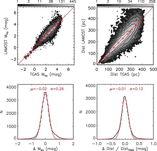
Comparison of absolute magnitudes and distances with those inferred from Gaia TGAS parallax for 50 000 LAMOST-TGAS common stars that have a TGAS-based magnitude error smaller than 0.2 mag. The upper panels shows colour-coded contours of stellar number density in logarithmic scale. Crosses in red are median values of our estimates calculated in bins of the TGAS-based values. The lower panels plot the distribution of differences of magnitudes and distances between our estimates and the TGAS-based values. Red lines are Gaussian fits to the distribution, with the mean and dispersion of the Gaussian marked in the plot.
Metal (iron) abundance [M/H] ([Fe/H]), α-element to metal (iron) abundance ratio [α/M] ([α/Fe]), as well as abundances of carbon and nitrogen, [C/H] and [N/H], are estimated using the LAMOST-APOGEE training set. Xiang et al. (2017) have demonstrated that the results have a precision comparable to those deduced from APOGEE spectra with the ASPCAP pipeline (García Pérez et al. 2016; Holtzman et al. 2015). Specifically, estimates of [M/H], [Fe/H], [C/H] and [N/H] have a precision better than 0.1 dex, given a spectral SNR high than 30, and ∼0.15 dex for a SNR of 20. We note, however, since the APOGEE stellar parameters are not externally calibrated except for [M/H], any systematics in the APOGEE results propagated into ours through the training set. As pointed out by Holtzman et al. (2015), APOGEE estimates of elemental abundances may suffer from systematic biases of about 0.1–0.2 dex. For [M/H], the APOGEE values are calibrated to [Fe/H] measurements of star clusters for [Fe/H] range [−2.5, 0.5] dex. Nevertheless, it is found that [Fe/H] ([M/H]) estimated with the LAMOST-APOGEE training set are systematically 0.1 dex higher than those estimated with the MILES library. Such an overestimation is also confirmed by examining common stars with high-resolution spectroscopic [Fe/H] measurements available from the PASTEL catalogue. The discrepancy is likely due to an offset in absolute value between the APOGEE and MILES (PASTEL) metallicities. The estimated [α/M] ([α/Fe]) values have a typical precision of 0.03–0.06 dex, given a spectral SNR higher than 20. Xiang et al. (2017) have demonstrated that as a consequence of such a high precision, a clear distinction between the sequences of thick and thin disc stars is seen in the [M/H] ([Fe/H])–[α/M] ([α/Fe]) plane, quite similar to that revealed by results from high-resolution spectroscopy. Note, however, that for stars with [α/M] higher than 0.30 dex or lower than 0.0 dex, the KPCA values are probably systematically underestimated or overestimated due to a lack of training stars of such abundance ratios. In addition, given that APOGEE [α/M] ([α/Fe]) values are not externally calibrated, there may also be some systematics hidden in our results.
4.4 Estimation of parameter errors
The method errors are deduced from the residuals obtained by applying the method to spectra of the template library or the training sets themselves. Both the mean and dispersion of the residuals are calculated and fitted as functions of Teff and [Fe/H], for dwarfs and giants separately. The mean reflects the bias induced by the method, and is thus corrected for all target stars. While the dispersion is combined with the error induced by the spectral noises to yield the final value of error of the estimated parameter of concern. In doing so, a grid of method errors (mean and dispersion) is first created in the Teff–[Fe/H] plane, and for a given set of atmospheric parameters of a target star, the corresponding value of method error is interpolated from the grid.
For log g estimated with the KPCA method using the LAMOST-Kepler training set, as well as metal/elemental abundances ([M/H], [Fe/H], [C/H], [N/H], [α/M], [α/Fe]) estimated using the LAMOST-APOGEE training set, since there are sufficiently large number of stars in common with the Kepler and APOGEE surveys that have not been included in the training samples, they can be used as the test samples (Xiang et al. 2017) to directly estimate the parameter errors. Given that no obvious trends with Teff, log g and [Fe/H] are seen, the errors are estimated as a function of spectral SNR only.
4.5 Specific flags
Specific flags are assigned to each star to better describe the quality of estimated parameters. A flag is assigned to describe the type of the best-matching template star. Based on the SIMBAD data base (Wenger et al. 2000), LSP3 template stars are divided into 38 groups, as listed in Table 3. While the majority template stars are normal (single) stars of A/F/G/K/M spectral types, there are also considerable numbers of spectroscopic binaries, double or multiple stars, variable stars, as well as of other rare types. The flag is set to help identify stars of specific type, although a careful analysis is essential to validate the results. The flag is an integer of value from 1 to 38, and is labelled, respectively, ‘TYPEFLAG_CHI2’ and ‘TYPEFLAG_CORR’ for results based on the minimum χ2 and correlation matching algorithms (Xiang et al. 2015b).
Types of template stars.
| Flag | Type | N |
|---|---|---|
| 1 | Normal star (single; AFGKM) | 757 |
| 2 | Pre-main-sequence star | 1 |
| 3 | L/T-type star | 9 |
| 4 | O/B-type star | 19 |
| 5 | S star | 6 |
| 6 | Carbon star | 5 |
| 7 | Blue supergiant star | 6 |
| 8 | Red supergiant star | 3 |
| 9 | Evolved supergiant star | 1 |
| 10 | Horizontal branch (HB) star (not including RCs) | 27 |
| 11 | Asymptotic giant branch (AGB) Star | 6 |
| 12 | Post-AGB star (proto-PN) | 4 |
| 13 | Planetary nebula (PN) | 1 |
| 14 | Star in nebula | 3 |
| 15 | Emission-line star | 2 |
| 16 | Pulsating variable star | 5 |
| 17 | Semiregular pulsating star | 22 |
| 18 | Classical Cepheid (delta Cep type) | 10 |
| 19 | Variable star of beta Cep type | 4 |
| 20 | Variable star of RR Lyr type | 5 |
| 21 | Variable star of BY Dra type | 28 |
| 22 | Variable star of RS CVn type | 12 |
| 23 | Variable star of alpha2 CVn type | 23 |
| 24 | Variable star of delta Sct type | 21 |
| 25 | Variable star of RV Tau type | 1 |
| 26 | Rotationally variable star | 4 |
| 27 | T Tau-type star | 1 |
| 28 | Flare star | 10 |
| 29 | Peculiar star | 4 |
| 30 | Long-period variable star | 13 |
| 31 | Spectroscopic binary | 80 |
| 32 | Eclipsing binary of Algol type (detached) | 7 |
| 33 | Eclipsing binary of beta Lyr type (semidetached) | 2 |
| 34 | Symbiotic star | 2 |
| 35 | Star with envelope of CH type | 7 |
| 36 | Variable star (unclassfied) | 78 |
| 37 | Double or multiple star | 79 |
| 38 | WD (DA) | 3 |
The second flag describes the correlation coefficient for radial velocity estimation. Although LSS-GAC intends to target stars that are identified as point sources in the photometry catalogues, there are still some contaminations from extragalactic sources (e.g. galaxies, QSOs), for which LSP3 gives problematic radial velocities because the pipeline treats all input spectra as stellar. In addition, radial velocity estimates can be problematic for stars of unusual spectra (e.g. of emission-line stars) or defective spectra (e.g. those seriously affected by cosmic rays and/or scatter light). In such cases, it is found that the peak correlation coefficient for radial velocity estimation is small compared to those of bulk stars. To mark those objects, a flag is assigned to each star in a way similar to the third flag in Xiang et al. (2015b), with the only difference that the current flag is set to be a positive float number, with negative ones replaced by 0.0. Experience suggests that one should treat the radial velocity cautiously if the flag has a value larger than 6.0. The flag is denoted by ‘VR_FLAG’ in the value-added catalogues. The peak correlation coefficient is also given by flag ‘PEAK_CORR_COEFF’.
Similar to the second flag of Xiang et al. (2015b), a flag is used to describe anomalies in the minimum χ2 of the best-matching spectral template. This flag is designed for parameters estimated with the weighted-mean algorithm. Again, the current flag is set to be a positive float, with negative values replaced by 0.0. The flag is denoted by ‘CHI2_FLAG’. The minimum χ2 of the best-matching template is presented as ‘MIN_CHI2’.
Another flag is assigned to indicate the quality of parameters estimated with the KPCA method. It is defined as the maximum value of the kernel function, dg, which reflects the minimum distance between the target and training spectra (Xiang et al. 2017). The flag is a float of value between 0.0 and 1.0, with larger values indicating better parameter estimates. All KPCA estimates that have a dg value smaller than 0.2 are not provided in the value-added catalogues due to their low reliability. The flag is labelled, respectively, ‘DG_MILES_TM’, ‘DG_MILES_G’, ‘DG_HIP’, ‘DG_KEP’ and ‘DG_APO’, for parameters estimated with the aforementioned different training sets, (cf. Table 5).
4.6 Recommended parameter values
Since different methods have been employed to deduce parameters Teff, log g, [Fe/H] and [α/Fe], one needs to choose between parameter values yielded by different methods for the specific problems that she/he may want to address. For this purpose, it is necessary to get to know both the advantages and limits of the individual methods employed.
For atmospheric parameters estimated with the weighted-mean algorithm, the advantage is that the results are found to be relatively insensitive to spectral SNR compared to results yielded by other methods. This implies that for low SNRs (e.g. <20), results from the weighted-mean method are more robust and should be preferred. A disadvantage of the method is that the resultant parameters suffer from some systematics, as described above. The advantage of parameters estimated with the KPCA method is that they are much less affected by systematics, and thus more accurate than the weighted-mean values, given sufficiently high spectral SNRs. A limitation is that they are available for limited ranges of parameters only, and, in addition, suffer from relatively large random errors at low SNRs.
We provide a recommended set of parameters {Teff, log g, MV, |$M_{K_{\rm s}}$|, [Fe/H], [α/Fe]} based on the above considerations. Table 4 lists the adopted methods for the recommended parameters and their effective parameter ranges. We emphasize that the recommended parameters are not necessarily the most accurate/precise ones. For example, although [Fe/H] values estimated with the KPCA method using the MILES library are adopted as the recommended values, those estimated using the LAMOST-APOGEE training set are, in fact, more precise. Values of Teff derived with the weighted-mean method are robust, but suffer from clustering effect, and are thus weakly clumped in the parameter space on the scale of a few tens of Kelvin. For [α/Fe], considering that there are systematic differences between the template matching and KPCA results (Xiang et al. 2017), our recommendation will lead to some level of inconsistency between the results for giants and dwarfs. For MV and |$M_{K_{\rm s}}$|, absolute magnitudes yielded using 300 PCs are adopted as the recommend values, but if the targets of interest are mainly composed of stars with low spectral SNRs (<30), one would better use the results from 100 PCs. In addition, because a cut of 0.2 is set for the maximum value of the kernel function, dg, to safeguard robust parameter estimates with the KPCA method (Xiang et al. 2017), about 18 per cent of the sample stars (mostly with very low SNRs) have no parameter estimates with the KPCA method. For those stars, the recommended parameters are not available. Rather than adopting the recommended values, we encourage users to make their own choice based on their specific problems under consideration.
Adopted methods and their effective parameter ranges for stellar parameter determinations.
| Parameter | Method | Effective range |
|---|---|---|
| Effective temperature | ||
| Teff_1 | Weighted-mean template matching | All |
| Teff_2 | KPCA with the MILES training set | |$T_{\rm eff}\_1 < 10\,000$| K |
| Teff (recommended) | Teff_1 | All |
| Surface gravity | ||
| Logg_1 | Weighted-mean template matching | All |
| Logg_2 | KPCA with the MILES training set | |$T_{\rm eff}\_1 < 10\,000$| K, |${\rm Logg\_1} > 3.0$| dex |
| Logg_3 | KPCA with the LAMOST-Kepler training set | |$T_{\rm eff}\_1 < 5600$| K, |${\rm Logg\_1} < 3.8$| dex or |${\rm Logg\_2} < 3.8$| dex |
| Logg (recommended) | Logg_1 | |$T_{\rm eff}\_1 > 10\,000$| K |
| Logg_3 | |$T_{\rm eff}\_1 < 5600$| K, |${\rm Logg\_1} < 3.8$| dex or |${\rm Logg\_2} < 3.8$| dex | |
| Logg_2 | Otherwise | |
| Metallicity | ||
| [Fe/H]_1 | Weighted-mean template matching | All |
| [Fe/H]_2 | KPCA with the MILES training set | |$T_{\rm eff}\_1 < 10\,000$| K |
| [Fe/H]_3 | KPCA with the LAMOST-APOGEE training set | |$T_{\rm eff}\_1 < 5600$| K, |${\rm Logg\_1} < 3.8$| dex or |${\rm Logg\_2} < 3.8$| dex |
| [Fe/H] (recommended) | [Fe/H]_1 | |$T_{\rm eff}\_1 > 10\,000$| K |
| [Fe/H]_2 | Otherwise | |
| α-element to iron abundance ratio | ||
| [α/Fe]_1 | Template matching using spectra of | |$4000 < T_{\rm eff}\_1 < 8000$| K |
| 3900–3980, 4400–4600 and 5000–5300 Å | ||
| [α/Fe]_2 | Template matching using spectra of | |$4000 < T_{\rm eff}\_1 < 8000$| K |
| 4400–4600 and 5000–5300 Å | ||
| [α/Fe]_3 | KPCA with the LAMOST-APOGEE training set | |$T_{\rm eff}\_1 < 5600$| K, |${\rm Logg\_1} < 3.8$| dex or |${\rm Logg\_2} < 3.8$| dex |
| [α/Fe] (recommended) | [α/Fe]_3 | |$T_{\rm eff}\_1 < 5600$| K, |${\rm Logg\_1} < 3.8$| dex or |${\rm Logg\_2} < 3.8$| dex |
| [α/Fe]_1 | Otherwise | |
| Other elemental abundances | ||
| [M/H] | ||
| [α/M] | KPCA with the LAMOST-APOGEE training set | |$T_{\rm eff}\_1 < 5600$| K, |${\rm Logg\_1} < 3.8$| dex or |${\rm Logg\_2} < 3.8$| dex |
| [C/H] | ||
| [N/H] | ||
| Absolute magnitudes | ||
| MV_1 | KPCA with the LAMOST-Hipparcos training set | |
| |$M_{K_{\rm s}}$|_1 | using 300 PCs | |$T_{\rm eff}\_1 < 12\,000$| K |
| MV_2 | KPCA with the LAMOST-Hipparcos training set | |
| |$M_{K_{\rm s}}$|_2 | using 100 PCs | |$T_{\rm eff}\_1 < 12\,000$| K |
| MV (recommended) | MV_1 | |
| |$M_{K_{\rm s}}$| (recommended) | |$M_{K_{\rm s}}$|_1 | |$T_{\rm eff}\_1 < 12\,000$| K |
For [M/H], [α/M], [C/H] and [N/H], since at the moment there is only one set of measurements, i.e. those with the KPCA method, they are simply adopted as the recommended values. Note that [M/H], [α/M], [C/H] and [N/H] are available only for stars of Teff < 5600 K and log g < 3.8 dex. Here Teff refers to that estimated with the weighted-mean method, while log g is either estimated with the weighted-mean method or by the KPCA method using the MILES stars as the training set.
Fig. 9 plots the stellar number density distributions in various planes of recommended parameters. In the Teff–log g and Teff–MV planes, the stars show two prominent clumps: one composed of FGK dwarfs and another of red clump stars. The compact contours of red clump stars indicate a high precision of the estimated parameters. Trajectories of stars in those planes are well consistent with the theoretical isochrones. Stars of [Fe/H] > −1.0 dex dominate the sample, indicating that most of the stars belong to the Galactic disc. The fraction of stars with [Fe/H] < −1.0 dex is only 1.8 per cent. Given the large difference between the numbers of metal-rich and metal-poor stars, even a small fraction of those metal-rich stars whose [Fe/H] estimates may have suffered large uncertainties could seriously contaminate the sample of metal-poor stars. This seems to have led to the appearance of a kinematically cold but metal-poor population in the [Fe/H]–Vr plane. One thus needs to be very careful when studying the metal-poor populations using this disc-star dominant sample. Comparison of [Fe/H] values derived with the weighted-mean and KPCA methods may help identify potential contaminators. Exercise shows that one excludes stars whose KPCA [Fe/H] estimates are smaller than the weighted-mean values by 0.3 dex, or replaces the estimates by the latter values; the artificial populations of cold, metal-poor stars in the [Fe/H]–Vr plane is largely disappeared.
![Contours of colour-coded stellar number density distributions in various planes of recommended parameters for the whole sample of stars in the value-added catalogues. Stellar isochrones in the Teff–log g and Teff–MV plots are from Rosenfield et al. (2016) and have a solar metallicity and an age of 4.5 Gyr. The left-hand and right-hand panels of third row are [Fe/H]–[α/Fe] plots showing the results for dwarfs and giants, respectively.](https://oup.silverchair-cdn.com/oup/backfile/Content_public/Journal/mnras/467/2/10.1093_mnras_stx129/3/m_stx129fig9.jpeg?Expires=1750294842&Signature=Gi5GTxsHQmbvBC~pmpG4OLXl50MG9adjuMxBh9HiNcNT~UWf9OHIIumh~EFsMwVYNaVE8DmT2LZhSpt2Yy3cE48QZ23eFEcEi9JxHwZCGijed~tacbxEP742DUKd5MBjFbcO7gkky1B71bYH6M2C4i9wblW4NSt~xUJ8dWuCz9IDgCCg7JIb~D2UiISnhD0r2BDLybaCf7s3qqoDopWU3ADmtFmbwftnJSeD3cYzEljRg4zHD0fndX8eWpX7dzfQ-UrdObGdF0nyxBiZ134lyeExBpaaU0MwymJMTWTQDqT1VvOsNvtFD0aDIt-52jbC7CClVmJfXdhdifRDXOJMtQ__&Key-Pair-Id=APKAIE5G5CRDK6RD3PGA)
Contours of colour-coded stellar number density distributions in various planes of recommended parameters for the whole sample of stars in the value-added catalogues. Stellar isochrones in the Teff–log g and Teff–MV plots are from Rosenfield et al. (2016) and have a solar metallicity and an age of 4.5 Gyr. The left-hand and right-hand panels of third row are [Fe/H]–[α/Fe] plots showing the results for dwarfs and giants, respectively.
Fig. 9 also shows that more metal-poor stars generally have higher [α/Fe] values. This is true for both dwarfs and giants, which is a natural consequence of the Galactic chemical evolution. For both dwarfs and giants, [α/Fe] values for stars of solar metallicity are close to zero. Nevertheless, [α/Fe] values of dwarfs and giants show different patterns. Dwarfs cover a wider range of [α/Fe] values than giants. There are very few giant stars of [α/Fe] < −0.2 dex or [α/Fe] > 0.3 dex. In contrast, there are quite a number of dwarfs of [α/Fe] < −0.3 dex or [α/Fe] > 0.4 dex. Moreover, besides the dominant thin disc sequence in the [α/Fe]–[Fe/H] plane, giants also exhibit an extra, weaker sequence of thick disc stars of a [α/Fe] value of ∼0.2 dex. This thick disc sequence is not seen in dwarfs. The larger random errors (Fig. 13) of [α/Fe] estimates for dwarfs are definitively an important reason for the absence of this sequence. Also, giants probe a larger volume than dwarfs as they are brighter. Thus, the giant sample contains more thick disc stars, whereas the dwarf sample is dominated by the local thin disc stars and young, hotter stars in the outer thin disc. In addition, and maybe more importantly, since different algorithms, spectral templates and wavelength ranges are used for [α/Fe] estimation for dwarfs and giants, and the results have not been calibrated externally using the data, for example, from high-resolution spectroscopy, systematic differences and errors may well be hidden in the [α/Fe] estimates of dwarfs and/or giants. A calibration of [α/Fe] estimates is an essential and urgent task for the future.
Fig. 10 plots distributions of stars in the Teff – log g, Teff – MV and (g − r, r) planes, colour-coded by [Fe/H]. The figure shows that amongst the cool stars, as expected, metal-rich ones generally have lower temperatures than those metal-poor ones. However, for hot stars, the derived metallicities show some strange patterns in the Teff–log g plane, which are not fully understood yet. A possible cause could be the inadequacy of parameter coverage of the MILES spectral library at higher temperatures. A further, detailed examination of log g estimates utilizing LAMOST-TGAS common stars, in particular for hot stars, is underway. On the whole, the trends of [Fe/H] seen in the Teff–MV and the (g − r, r) planes seem to be reasonable. The brighter side of the (g − r, r) diagram is dominated by metal-rich stars as they represent a local, thin disc sample. On the other hand, at the fainter side of the diagram, one sees that metal-rich stars are, in general, redder, while the metal-poor ones are bluer. Again, this is what one would expect.
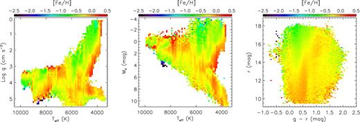
Distributions of sample stars in Teff–log g, Teff–MV and (g − r, r) diagrams colour-coded by median metallicity, defined as the median value of stars in bins of 100 K × 0.1 dex in Teff–log g, 100 K × 0.2 mag in Teff–MV and 0.05 × 0.1 mag in (g − r, r) plane, respectively, for the three panels from left to right.
Fig. 11 plots error distributions of recommended parameter estimates. Spectral SNR is the main factor that determines the amount of parameter error, and stars of different spectral types have also different parameter errors. A detailed analysis of how the parameter errors depends on spectral SNR and stellar parameters can be found in Xiang et al. (2015b, 2017). Most of the stars have a radial velocity error of a few km s−1. However, some of them, mostly hot stars of low SNRs, have errors reaching 20 km s−1. Temperature errors are around 100 K for most stars, but those of hot ones reach 400–600 K. The large temperature errors for hot stars are mainly caused by the small number and large parameter uncertainties of hot stars in the MILES library. Similar trend is seen in [Fe/H] errors, where most stars have an error between 0.1 and 0.2 dex. However, the error distribution exhibits a second peak at 0.5–0.6 dex, mainly contributed by hot stars. Errors of log g typically have values of 0.1–0.2 dex, with a small fraction reaching 0.3–0.4 dex. Errors of MV can be as small as 0.2 mag at high spectral SNRs, but reach 0.8–1.0 mag at low SNRs (∼10). MV values estimated using 100 PCs have larger errors compared to those deduced using 300 PCs, but they are less sensitive to SNR, and have errors of 0.6–0.8 mag at low SNRs (∼10). Errors of |$M_{K_{\rm s}}$| have similar trends. Errors in [α/Fe] show two populations. The lower one is of giants, which has values of 0.02–0.09 dex. The higher one is of dwarfs, and has values of 0.09–0.25 dex, peaking around 0.1 dex. Note that as discussed above, since the results are not calibrated by independent, external data sets, there could be systematic uncertainties in [α/Fe] estimates that have not been included in the current error estimates. This is particularly true for giant stars, for which the quoted errors are very small. Errors of [C/H] and [N/H] estimates range from 0.05 to 0.20 dex, with most of them smaller than 0.15 dex.
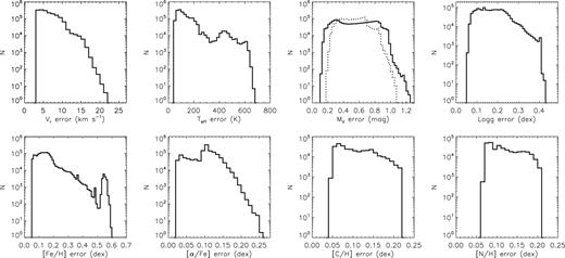
Error distributions of recommended parameter estimates. For MV, error distribution of the other set of MV estimates deduced using 100 PCs is shown by a dotted line.
A comparison of recommended stellar atmospheric parameters with LSS-GAC DR1 for the whole LSS-GAC DR1 sample is shown in Fig. 12. The figure shows that Teff estimates from the two data releases are quite consistent. For log g, the plot shows significant patterns. Similar patterns are seen by comparing LSS-GAC DR1 log g estimates with asteroseismic measurements (Ren et al. 2016). The causes of such patterns are discussed in Xiang et al. (2017), and are essentially due to the inadequacies of log g estimates in LSS-GAC DR1 ones. On the whole, new [Fe/H] estimates show good correlation with those of LSS-GAC DR1. The standard deviation of the two sets of [Fe/H] estimates of the whole sample is 0.15 dex. However, the current estimates are systematically 0.05 dex lower than LSS-GAC DR1. There is also a group of stars whose new [Fe/H] values are significantly higher than those of LSS-GAC DR1. In addition, the sharp boundary seen in the LSS-GAC DR1 results now disappears. Again, the causes of these differences are discussed in Xiang et al. (2017), and are mainly due to the inadequacies of [Fe/H] estimates in LSS-GAC DR1.
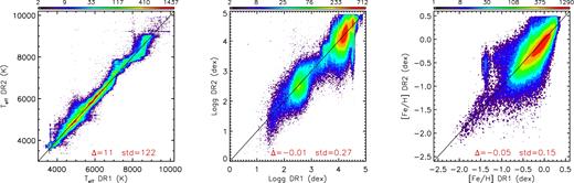
Comparison of the new recommended stellar atmospheric parameters with those of LSS-GAC DR1. Mean and standard deviations of the parameter differences between DR2 and DR1 are marked in the plot.
5 REPEAT OBSERVATIONS
About 28 per cent of stars in the value-added catalogues have repeat observations. The repeat observations are valuable for various purposes, including (1) time-domain spectroscopy, (2) robustness check of parameter estimates, (3) improvement of stellar parameter estimates by averaging repeat measurements, etc. Fig. 13 plots the distribution of number of stars as a function of number of repeat observations per object, as well as the distribution of time separations of repeat observations. Stellar number decreases approximately linearly with the increasing number of repeat observations. There are 95 350 unique stars that are observed three times or more, and 5460 unique stars that are observed five times or more. Time separation covers a range from a few hours to nearly 1000 d. Most repeat observations occurred in the same night, when different plates that shared the same central bright stars or adjacent plates that had overlapping fields of views were observed. Note that, to better present the data, the horizontal axis of the figure has been chosen to artificially start from 0.8 d, but the real time separation in the first bin was smaller than 4 h due to hour angle limitations of LAMOST (Cui et al. 2012). Note also that here repeat observations refer to those taken with different plates. In fact, each plate observed usually has two to three exposures. The current analysis is based on co-added spectra of those adjacent individual exposures. Further, independent treatment of the individual exposures of each plate observed in the future will significantly increase the repeat observation rate in the sense that every star targeted has at least one repeat observation, separated by tens of minutes.
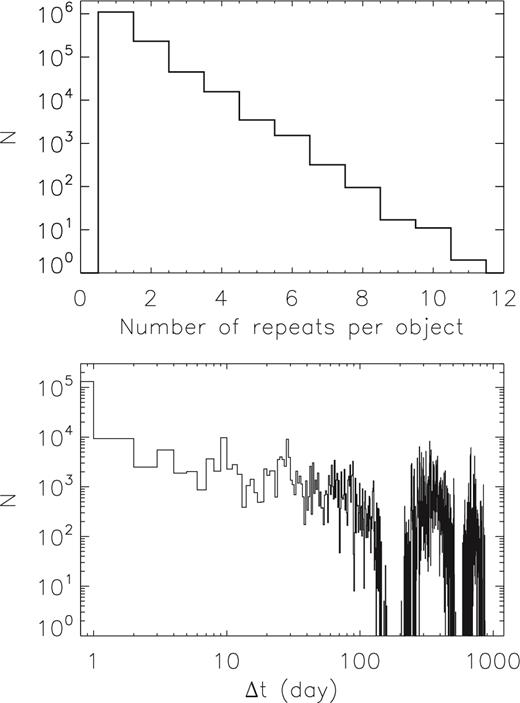
Upper panel: stellar numbers as a function of number of repeat observations per object. Lower panel: distribution of time separation for repeat observations.
Some systematic studies utilizing repeat observations are underway. As an example, Fig. 14 shows the spectra in the 3900–4400 Å wavelength range of two stars with repeat observations. The data clearly show shifts of spectral line positions, thus radial velocity variations. The first example has an amplitude of radial velocity variations larger than 180 km s−1. The offsets of repeat observations from the first one are, respectively, 3.994 11, 4.023 74, 4.046 00 72.855 50 and 76.767 793 d. Effective temperatures estimated from the six observations are, respectively, 4931, 5192, 5150, 5182, 5507 and 4953 K, MV absolute magnitudes are 6.10, 5.89, 5.82, 5.43, 5.42 and 6.56 mag, and [Fe/H] metallicities are −0.22, −0.33, −0.24, −0.34, −0.15 and −0.07 dex. The second example star has a radial velocity variation amplitude larger than 60 km s−1. The offsets of repeat observations from the first one are, respectively, 0.034 47, 346.023 93, 346.063 02, 374.905 49, 374.944 06 and 374.987 18 d. Teff estimates from the seven observations are, respectively, 5349, 5340, 5046, 5258, 5512, 5512 and 5526 K, the MV absolute magnitudes are 4.47, 4.29, 4.62, 4.49, 4.74, 4.79 and 4.76 mag, and [Fe/H] metallicities are −0.11, −0.05, 0.03, 0.00, −0.04, −0.03 and −0.04 dex. It seems that in addition to the radial velocity variations, the two stars also exhibit significant variations in effective temperature and absolute magnitude. Further analyses are, however, required to reveal the nature of the variations.
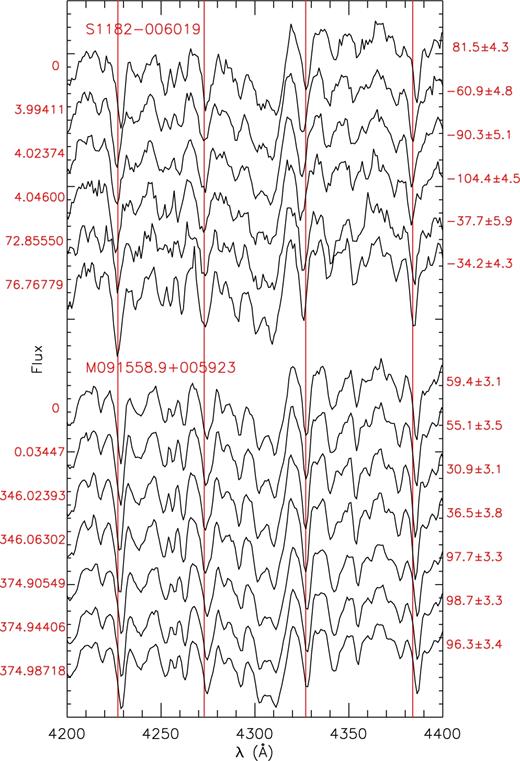
Examples of spectra of wavelength range of 4200–4400 Å of two stars with repeat observations. Numbers on the left are JD offsets with respect to the first observation, while numbers on the right are radial velocity measurements. Object ID from the input catalogues are marked on the plot.
A detailed robustness examination on the LSP3 stellar parameters using repeat observations can be found in Xiang et al. (2015b) for radial velocity measurements and atmospheric parameter determinations with the weighted-mean method, and in Xiang et al. (2017) for atmospheric parameters estimated with the KPCA method. Fig. 15 plots the dispersions of differences of recommended parameters deduced from repeat observations that have comparable SNRs (20 per cent) as a function of SNR. The dispersions represent random errors of the parameters induced by spectral noises. For this purpose, values of dispersions shown in the figure have been divided by square root of 2. Results for giants, hot (Teff > 7000 K) and cool (Teff <7000 K) dwarfs are shown separately. Generally, hot dwarfs have larger random errors in Vr, Teff, [Fe/H] and [α/Fe] estimates. For all parameters, the random errors are quite sensitive to SNR. Given an SNR higher than 100, random errors of radial velocities induced by spectral noises for cool stars can be as small as 1–2 km s−1, and the values are 3–4 km s−1 for hot stars. For an SNR of 10, the errors increase to 5–10 km s−1 for cool stars, and 20 km s−1 for hot stars. Note that the final error estimates of Vr have been set to a minimum value of 3 km s−1 to account for the potential systematic uncertainties, which is ∼2 km s−1, as estimated via external examinations using the LAMOST-APOGEE common stars. As introduced in Section 4.4, for all stellar parameters, these random errors and their trends of variations with spectral SNR, Teff and [Fe/H] have been incorporated into the final error estimates, which also include uncertainties induced by the inadequacies of the parameter estimation methods for both giants and dwarfs.
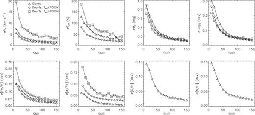
Random errors of recommend parameters as a function of spectral SNR as deduced by comparing results from repeat observations. Results for giants, hot and cool dwarfs are shown separately.
6 EXTINCTION AND DISTANCE
6.1 Extinction
Similar to LSS-GAC DR1 (Yuan et al. 2015), various techniques are employed to estimate the interstellar reddening towards the individual stars. The methods include the star-pair technique, comparing observed colours with synthetic ones from stellar model atmospheres, as well as a method based on the stellar colour loci.
The star-pair method assumes that stars with identical stellar atmospheric parameters (Teff, log g, [Fe/H]) have the same intrinsic colours. Thus, for a reddened star, its intrinsic colours can be inferred from its pairs/counterparts with either nil or well-known extinction (Yuan et al. 2015). The method is straightforward, and, moreover, free from stellar model atmospheres. To derive extinction with this method, a control sample with nil or well-known extinction is inherited from LSS-GAC DR1. The control sample contains low-extinction stars whose E(B − V) values can be well approximated by the reddening map of Schlegel, Finkbeiner & Davis (1998, hereafter SFD98). For a given target star, the E(B − V) is then derived by fitting g − r, r − i, i − J, J − H and H − Ks optical to the infrared colours simultaneously by the corresponding values of the pair stars in the control sample, assuming the universal extinction coefficients of Yuan, Liu & Xiang (2013). When available, g-, r-, i-band magnitudes from the XSTPS-GAC survey (Zhang et al. 2013, 2014; Liu et al. 2014) are used, otherwise they are taken from the APASS survey (Munari et al. 2014) or from the SDSS survey (DR8; Aihara et al. 2011) for a few B/M/F plates of high Galactic latitudes. J, H, Ks magnitudes are from the 2MASS survey (Skrutskie et al. 2006). There are a few (∼3–5 per cent) stars for which different colours yield quite different reddenings. For those stars, either the photometry or the stellar atmospheric parameters or both are problematic. It is found that in such cases, E(B − V) is often overestimated by a significant amount. To account for this, if g − r and r − i colours of a given star yield reddening of different signs and yield values differed by more than 0.2 mag, the resultant E(B − V) estimate is discarded. The corresponding entry in the value-added catalogues are set to −9. Comparison with the SFD98 reddening map for high Galactic latitude regions of low extinction illustrates a typical uncertainty of 0.036 mag for E(B − V) thus estimated (Fig. 16), which is similar to that of LSS-GAC DR1. Note that we use the recommended atmospheric parameters for reddening estimation. Different results are expected if different sets of atmospheric parameters are adopted. Nevertheless, given the good precision of the current parameter estimates, the differences are small. For example, E(B − V) values derived using atmospheric parameters estimated with the weighted-mean algorithm differ from the default results by a dispersion of only ∼0.01 mag. E(B − V) thus estimated is denoted by ‘EBV_SP’ in the value-added catalogues.
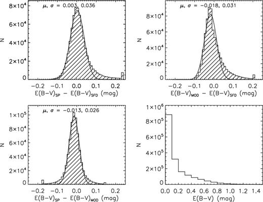
Distributions of differences of E(B − V) estimated by different methods or from the SFD98 map except for the bottom right-hand panel where the distribution is for the adopted values of E(B − V) for all stars in LSS-GAC DR2. E(B − V)SP and E(B − V)MOD denote, respectively, the values derived from the star-pair and stellar model atmosphere methods, whereas E(B − V)SFD refers to values extracted from the two-dimensional reddening map of SFD98. The comparisons are for stars of |b| > 15° and E(B − V)SFD < 0.3 mag only.
E(B − V) values have also been determined by comparing photometric colours with synthetic ones. In doing so, a grid of synthetic colours is first constructed by convolving the synthetic spectra of Castelli & Kurucz (2004) with the transmission curves of filters for the photometric systems of SDSS3 (Gunn et al. 1998; Doi et al. 2010) and 2MASS4 (Milligan, Cranton & Skrutskie 1996). Synthetic colours for a star of given atmospheric parameters Teff, log g and [Fe/H] are then deduced by linearly interpolating the grid. E(B − V) is then estimated as the weighted mean of values inferred from the individual colours, weighted by the reddening coefficients of Yuan et al. (2013). As Fig. 16 shows, E(B − V) values thus derived have a precision of about 0.03 mag, but are found to be systematically lower than the values given by either the star-pair method or by the SFD98 map, by 0.01–0.02 mag. The underestimation is likely to be caused by the slight different temperature scales between the LSP3 and Kurucz atmospheric models. As pointed out above, LSP3 temperatures are calibrated to the metallicity-dependent colour–temperature relations of Huang et al. (2015c), constructed using a sample of stars with Teff estimated directly from angular diameters measured with interferometry and the trigonometric parallaxes from the Hipparcos Satellite. It is found that the relations of Huang et al. (2015c) yield temperatures generally ∼100 K lower than earlier results in the literature. E(B − V) estimated with this method is denoted ‘EBV_MOD’ in the catalogues.
Finally, extinction values deduced from multiband photometry by fitting the stellar colour loci (Chen et al. 2014) are also included in the catalogues. Results from this method are currently available only for stars within the footprint and magnitude range of XSTPS-GAC, i.e. for stars targeted by the LSS-GAC main and M31/M33 surveys. As shown by Yuan et al. (2015), the method yields an E(B − V) precision of about 0.07 mag and works best for dwarf stars. E(B − V) thus estimated is denoted by ‘EBV_PHOT’ in the catalogues.
Considering that the star-pair method is model free, and often achieves a better precision compared to other methods, E(B − V) yielded by the method (‘EBV_SP’) are generally adopted as the recommended values. Considering that there are few hot stars in the control sample used by the star-pair method, ‘E(B-V)_MOD’ is adopted as the recommended for stars hotter than 9000 K. Since the SFD98 map is a two-dimensional one, it provides an upper limit of E(B − V) for reddening towards the individual Galactic stars. Based on this consideration, if the E(B − V) value of a star deduced from the star-pair method or from the method based on model atmospheres excess the SFD98 value by 0.1 mag (∼3σ), the latter is adopted as the recommended value. The distribution of adopted E(B − V) values for all stars in LSS-GAC DR2 are shown in the bottom right-hand panel of Fig. 16. With E(B − V) determined, values of interstellar extinction in the individual photometric bands can be easily computed using the extinction coefficients available from, for example, Yuan et al. (2013).
6.2 Distance
Distance to individual stars are also estimated with a variety of methods. One is to infer from the absolute magnitudes derived directly from the LAMOST spectra with the KPCA method using the LAMOST-Hipparcos training set. In doing so, if photometric magnitudes of all g, r and Ks bands have an error smaller than 0.1 mag, and are not saturated, then both MV and |$M_{K_{\rm s}}$| are used to calculate a weighted-mean distance by taking the inverse squared magnitude errors as weights, otherwise only bands with good photometry are utilized to infer the distance. Generally, Ks band contributes a larger weight as it suffers from much less severe extinction than Vband. The V-band photometry is transformed from g and r magnitudes using the equation of Jester et al. (2005). Errors of absolute magnitudes, extinction and photometry are all incorporated in the estimation of distance errors. Note that it is found that the estimated MV and |$M_{K_{\rm s}}$| are not independent quantities but largely correlated with each other, so that when estimating errors for the weighted-mean distance, we simply adopt the weighted-mean distance errors in the individuals bands rather than inferring from the reduced variance as done for the independent measurements. This may have overestimated the distance errors to some extent. Distance estimated with this method is denoted as ‘DIST_SP1’ and ‘DIST_SP2’ in the value-added catalogues for results inferred from absolute magnitudes using 300 and 100 PCs, respectively.
Another method to estimate stellar distance is based on empirical relations between the absolute magnitudes and stellar atmospheric parameters constructed utilizing the MILES stars. A detailed description of the derivation of the empirical relations is presented in (Yuan et al. 2015). Here, since the atmospheric parameters of MILES stars have been re-determined/calibrated (cf. Section 4.1), the relations are updated accordingly. The new relations have much smaller residuals – with dispersions of g- (and r-) band absolute magnitudes of only about 0.08, 0.13, 0.15 and 0.20 mag for OBA stars, FGK dwarfs, KM dwarfs and GKM giants, respectively. The corresponding residuals in the 2MASS infrared bands are about 0.15, 0.26, 0.06 and 0.26 mag. The small residuals suggest that the method is robust. Errors of absolute magnitudes thus derived for the individual LSS-GAC stars are mainly contributed by uncertainties of the stellar atmospheric parameters. Here, both the recommended atmospheric parameters and atmospheric parameters yielded by the weighted-mean algorithm are used to estimate absolute magnitudes. To obtain realistic error estimates of absolute magnitudes, we adopt a Monte Carlo strategy to propagate the errors of stellar atmospheric parameters. The distance errors are then estimated taking into account contributions by errors in absolute magnitudes, extinction and photometry. Distances estimated with this method using the recommended parameters are denoted as ‘DIST_EM1’ in the value-added catalogues, and those using the weighted-mean atmospheric parameters are denoted as ‘DIST_EM2’. In addition, stellar distances derived from photometry by Chen et al. (2014) via fitting stellar colour loci, if available, are also presented in the value-added catalogues, and are denoted by ‘DIST_PHOT’.
Estimating distance using absolute magnitudes derived directly from the LAMOST spectra does not depend on stellar model atmospheres and stellar atmospheric parameters, and thus are expected to suffer from minimal systematics. Comparison with distances inferred from the Gaia TGAS parallaxes (Fig. 8) demonstrates that the overall systematic errors in our inferred distances are negligible, and the random errors can be as small as ∼10 per cent, given high enough spectral SNRs. Uncertainties in absolute magnitude thus distance estimates are sensitive to spectral SNRs. For an SNR of 10, the uncertainty increases to 30–40 per cent. Fig. 17 further shows that distance estimates from absolute magnitudes derived using both 300 and 100 PCs have essentially negligible (1–2 per cent) systematic errors at all Teff in the range of 5000–9000 K. Note that to incorporate stars in a wide temperature range for the comparison, especially for the high-temperature end, here we have adopted an error cut of 0.3 mag for the TGAS-based magnitudes instead of 0.2 mag as adopted for Fig. 8. As a result, the dispersion become 14 per cent, which is larger than 12 per cent shown in Fig. 8. While for stars cooler than 5000 K, our distances seem to be underestimated by 5–10 per cent. The figure also shows that distances yielded by the empirical relations using the recommended parameters are systematically underestimated by about 11 per cent, and the systematics show moderate dependence on Teff. Such an underestimation is probably caused by either hidden systematic errors in the stellar atmospheric parameters, especially log g, or by systematic errors in the empirical relations. Note that although the current parameter estimates achieved high precisions, potential systematic errors could be existed, which are probably a few tens of Kelvin in Teff, a few per cent to 0.1 dex in log g and a few per cent to 0.1 dex in [Fe/H]. Potential systematic errors for metal-poor stars ([Fe/H] < −1.0 dex) are likely larger and should be treated cautiously. Distances yielded by the empirical relations using the weighted-mean parameters are systematically overestimated by 6 per cent, and there are strong patterns.
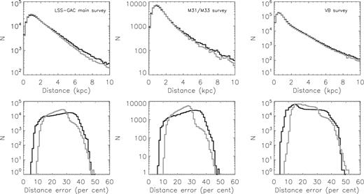
Distributions of distances and errors of stars targeted by the LSS-GAC main (left-hand panel), M31/M33 (middle panel) and VB (right-hand panel) surveys. Black and grey lines represent distances inferred from absolute magnitudes derived from LAMOST spectra with the KPCA method using 300 and 100 PCs, respectively.
Distances inferred from absolute magnitudes directly determined from the LAMOST spectra using 300 PCs (‘DIST_SP1’) are currently adopted as the recommended values. It is emphasized that users should choose a proper set according to their own problems of interest. Fig. 18 plots the distributions of distances and error estimates for ‘DIST_SP1’ and ‘DIST_SP2’ for LSS-GAC DR2 stars of the main, M31/M33 and VB surveys, respectively. The distances peak at about 1 kpc, but with a few beyond 10 kpc. For the whole sample, 22, 5 and 2 per cent of the stars have a distance larger than 2, 5 and 10 kpc, respectively. The quoted errors have a wide distribution from ∼7 to >40 per cent. For ‘DIST_SP1’, about 11.5, 25.5, 63.0 and 98.8 per cent of the stars have a quoted error smaller than 15, 20, 30 and 40 per cent, respectively. The numbers are, respectively, 4.6, 22.9, 87.8 and 99.7 per cent for distances inferred from absolute magnitudes derived using 100 PCs. Finally, note that as mentioned in Section 4, there are about 18 per cent of stars that the KPCA method has failed to provide reliable estimates of absolute magnitudes due to low spectral SNRs. For those stars, the recommend distances are not available, while as a compromise, one may use the distance derived with the empirical relations utilizing the weighted-mean atmospheric parameters.
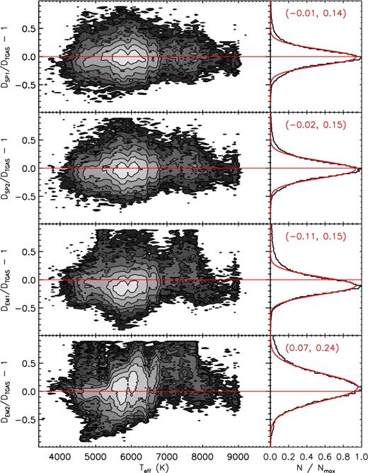
Percentage differences of distances between our estimates and those inferred from Gaia TGAS parallax as a function of the recommended Teff for a sample of 100 000 common stars. For up to low, the four panels show results for our distance estimates inferred from absolute magnitudes derived from LAMOST spectra using 300 PCs (first panel), 100 PCs (second panel) and from absolute magnitudes estimated using empirical relations utilizing the recommended parameters (third panel) and the weighted-mean parameters (fourth panel). An error cut of 0.3 mag in the TGAS-based magnitudes is applied.
Fig. 19 plots the density distributions of LSS-GAC DR2 stars in the Galactic X–Y and X–Z planes for the main, M31/M33 and VB surveys, separately. Here, the X, Y and Z are calculated assuming R⊙ = 8.0 kpc and Z⊙ = 0 kpc, and the recommended distances are used for the calculation. The figure shows that the main survey samples the outer disc well, while the VB survey samples the local disc very well. Some stars are located beyond 20 kpc in the anticentre direction and some are beyond 10 kpc in the vertical direction.
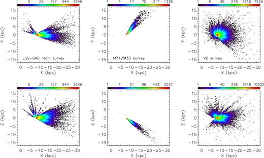
Colour-coded stellar density distributions in the Galactic X–Y and X–Z planes for stars targeted by the LSS-GAC main (left-hand panel), M31/M33 (middle panel) and VB (right-hand panel) surveys.
7 MULTIBAND PHOTOMETRY, PROPER MOTION AND ORBITAL PARAMETERS
Multiband photometry from the far-UV to the mid-IR, including magnitudes in FUV and NUV bands from the GALEX (Martin et al. 2005), g, r, i bands from the XSTPS-GAC, SDSS and APASS, J, H, Ks bands from the 2MASS, and w1, w2, w3, w4 bands from the WISE (Wright et al. 2010), are included in the value-added catalogues using with a 3 arcsecond match radius for source cross-identifications.
Proper motions for LSS-GAC stars from UCAC4 (Zacharias et al. 2013) and PPMXL (Roeser, Demleitner & Schilbach 2010), as well as those derived by combing the XSTPS-GAC and 2MASS catalogues (Yuan et al. 2015), are also included in the value-added catalogues.
Given celestial position, distance, radial velocity and proper motions, the stellar orbital parameters, including eccentricity, epicentre and pericentre radii, minimum and maximum vertical distances from the disc are computed assuming a simple, axisymmetric Galactic potential as presented in table 1 of Gardner & Flynn (2010). The Sun is assumed to be located at (X, Y, Z) = (−8, 0, 0) kpc, and the local standard of rest has values (U⊙, V⊙, W⊙) = (7.01, 10.13, 4.95) km s−1 (Huang et al. 2015b). When calculating the orbital parameters, systematic trends in proper motions with celestial positions are corrected for using the relations presented in Carlin et al. (2013) and in Huang et al. (2015b) for PPMXL and UCAC4 proper motions, respectively. Note that the systematics in proper motions have also been found to correlate with colour and magnitudes (e.g. Sun et al. 2015; Yuan et al. 2015). Such systematics have not been accounted for in the current treatment. Fig. 20 shows the eccentricity distribution of the sample stars.
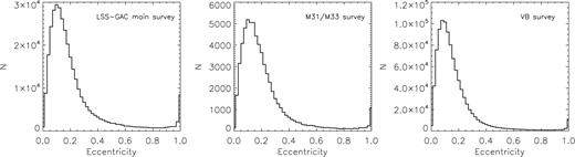
Distributions of orbital eccentricities for stars targeted by the LSS-GAC main (left-hand panel), M31/M33 (middle panel) and the VB (right-hand panel) surveys.
8 FORMAT OF THE VALUE-ADDED CATALOGUES
Similar to LSS-GAC DR1, this second release of value-added catalogues are stored in three binary tables in FITS format. The filenames are ‘lss-gac_dr2_GAC.fits’, ‘lss-gac_dr2_M31.fits’ and ‘lss-gac_dr2_VB.fits’, corresponding to the LSS-GAC main, M31/M33 and VB surveys, respectively. The value-added catalogues include information of the LAMOST observations, stellar parameters and error estimates, interstellar reddening, distance, multiband photometry, as well as proper motions and orbital parameters for 1790 633 observations of 1393 844 unique stars that have a spectral SNR(4650 Å) higher than 10. A detailed description of the catalogue content is presented in Table 5 . Note that compared to LSS-GAC DR1, more information about the observations and stellar parameter estimates is provided for a better description of the data. This includes, for example, information of Julian date at the start of the first exposure, airmass, lunar distance, as well as telescope altitude and so on. Stellar type of the best-matching template is also provided, which should be helpful for identifying stars of special interest (cf. Section 4.5). The catalogues are accessible from http://lamost973.pku.edu.cn/site/data along with a descriptive readme.txt file.
Description of the second release of LSS-GAC value-added catalogues.
| Col. | Name | Description |
|---|---|---|
| 1 | spec_id | LAMOST unique spectral ID, in format of date-plateid-spectrographid-fibreid |
| 2 | date | Date of observation |
| 3 | plate | LAMOST plate ID, not necessarily unique |
| 4 | sp_id | LAMOST spectrograph ID, ranging from 1 to 16 |
| 5 | fibre_id | LAMOST fibre ID for a given spectrograph, ranging from 1 to 250 |
| 6 | objid | Object ID in the input catalogues |
| 7 | objtype | Initial object type from the survey input catalogues |
| 8 | ra | Right ascension of J2000.0 (°) |
| 9 | dec | Declination of J2000.0 (°) |
| 10 | l | Galactic longitude (°) |
| 11 | b | Galactic latitude (°) |
| 12 | jd | Julian days at the middle time of the first exposure |
| 13 | moonphase | Moon phase at the middle time of the first exposure |
| 14 | monodis | Moon distance at the middle time of the first exposure |
| 15 | airmass | Airmass at the middle time of the first exposure |
| 16 | alt | Altitude (in degrees) of the telescope at the middle time of the first exposure |
| 17 | az | Azimuth angle (in degrees) of the telescope at the middle time of the first exposure |
| 18 | ha | Hour angle (in degrees) of the telescope at the middle time of the first exposure |
| 19 | badfiber | Is it a bad fibre? (yes – 1, no – 0) |
| 20 | satflag | Is the spectrum saturated? (yes – 1, no – 0) |
| 21 | brightflag | Are there bright stars (snr_b > 300) in the nearby five fibres (yes – 1, no – 0) |
| 22 | brightsnr | Largest snr_b in the nearby five fibres |
| 23 | object_sky_ratio | Object to sky flux ratio |
| 24 | snr_b | S/N(4650 Å) per pixel |
| 25 | snr_r | S/N(7450 Å) per pixel |
| 26 | uqflag | Uniqueness flag. If the target has been observed n times, then uqflag runs from 1 to n, with 1 denoting |
| the spectrum of the highest snr_b | ||
| 27 | vr | Radial velocity yielded by LSP3, after corrected for a systematic offset of −3.1 km s−1 (km s−1) |
| 28 | err_vr | Error of radial velocity yielded by LSP3 (km s−1) |
| 29 | teff | Recommended Teff (K) |
| 30 | err_teff | Error of the recommended Teff |
| 31 | teff_from | Which method is the recommended Teff adopted |
| 32 | logg | Recommended log g (cm s−2) |
| 33 | err_logg | Error of the recommended log g |
| 34 | logg_from | Which method is the recommended log g adopted |
| 35 | mv | Recommended absolute magnitude in V band |
| 36 | err_mv | Error of MV |
| 37 | mv_from | Which method is the recommended MV adopted |
| 38 | mk | Recommended absolute magnitude in Ks band |
| 39 | err_mk | Error of |$M_{K_{\rm s}}$| |
| 40 | mk_from | Which method is the recommended |$M_{K_{\rm s}}$| adopted |
| 41 | feh | Recommended [Fe/H] (dex) |
| 42 | err_feh | Error of the recommended [Fe/H] |
| 43 | feh_from | Which method is the recommended [Fe/H] adopted |
| 44 | afe | Recommended [α/Fe] (dex) |
| 45 | err_afe | Error of the recommended [α/Fe] |
| 46 | afe_from | Which method is the recommended [α/Fe] adopted |
| 47 | am | α-element to metal abundance ratio [α/M] estimated by training the LAMOST-APOGEE stars (dex) |
| 48 | err_am | Error of [α/M] |
| 49 | mh | Metal abundance [M/H] estimated by training the LAMOST-APOGEE stars (dex) |
| 50 | err_mh | Error of [M/H] |
| 51 | ch | Carbon abundance [C/H] estimated by training the LAMOST-APOGEE stars (dex) |
| 52 | err_mh | Error of [C/H] |
| 53 | nh | Nitrogen abundance [N/H] estimated by training the LAMOST-APOGEE stars (dex) |
| 54 | err_nh | Error of [N/H] |
| 55 | ebv | Recommended E(B − V) |
| 56 | dist | Recommended distance (pc) |
| 57 | err_dist | Error of the recommended distance |
| 58 | dist_from | Which method is the recommended distance adopted |
| 59 | vr_peak_corr_coeff | Peak correlation coefficient for radial velocity estimation |
| 60 | vr_flag | Flag to describe value of ‘vr_peak_corr_coeff’, n means the vr_peak_corr_coeff |
| is smaller than the median value of the sample stars with the same snr_b by n ×MAD | ||
| 61 | teff1 | Teff estimated with the weighted-mean algorithm (K) |
| 62 | err_teff1 | Error of teff1 |
| 63 | teff2 | Teff estimated with the KPCA method (K) |
| 64 | err_teff2 | Error of teff2 |
| 65 | logg1 | Log g estimated with the weighted-mean algorithm (cm s−2) |
| 66 | err_logg1 | Error of logg1 |
| 67 | logg2 | Log g estimated with the KPCA method using MILES stars as training set (cm s−2) |
| 68 | err_logg2 | Error of logg2 |
| 69 | logg3 | Log g estimated with the KPCA method using LAMOST-Kepler stars as training set (cm s−2) |
| 70 | err_logg3 | Error of logg3 |
| 71 | mv1 | MV estimated with the KPCA method taking LAMOST-Hipparcos stars as training set using 300 PCs (mag) |
| 72 | err_mv1 | Error of mv1 |
| 73 | mv2 | MV estimated with the KPCA method taking LAMOST-Hipparcos stars as training set using 100 PCs (mag) |
| 74 | err_mv2 | Error of mv2 |
| 75 | mk1 | |$M_{K_{\rm s}}$| estimated with the KPCA method taking LAMOST-Hipparcos stars as training set using 300 PCs (mag) |
| 76 | err_mk1 | Error of mk1 |
| 77 | mk2 | |$M_{K_{\rm s}}$| estimated with the KPCA method taking LAMOST-Hipparcos stars as training set using 100 PCs (mag) |
| 78 | err_mk2 | Error of mk2 |
| 79 | feh1 | [Fe/H] estimated with the LSP3 weighted mean algorithm (dex) |
| 80 | err_feh1 | Error of feh1 |
| 81 | feh2 | [Fe/H] estimated with the LSP3 KPCA method by training the MILES stars (dex) |
| 82 | err_feh2 | Error of feh2 |
| 83 | feh3 | [Fe/H] estimated with the LSP3 KPCA method by training the LAMOST-APOGEE stars (dex) |
| 84 | err_feh3 | Error of feh3 |
| 85 | afe1 | [α/Fe] estimated by template matching with synthetic spectra using spectral segments |
| of 3900–3980, 4400–4600 and 5000–5300 Å (dex) | ||
| 86 | err_afe1 | Error of afe1 |
| 87 | afe2 | [α/Fe] estimated by template matching with synthetic spectra using spectral segments |
| of 4400–4600 and 5000 – 5300 Å (dex) | ||
| 88 | err_afe2 | Error of afe2 |
| 89 | afe3 | [α/Fe] estimated with the LSP3 KPCA method using the LAMOST-APOGEE training set (dex) |
| 90 | err_afe3 | Error of afe3 |
| 91 | besttemp_chi2 | Name of the best-matching template star with χ2 algorithm |
| 92 | besttemp_corr | Name of the best-matching template star with correlation algorithm |
| 93 | typeflag_chi2 | Stellar types of the best-matching template star with χ2 algorithm |
| 94 | typeflag_corr | Stellar types of the best-matching template star with correlation algorithm |
| 95 | min_chi2 | Minimum χ2 yielded by LSP3 from template matching with the MILES library |
| 96 | chi2_flag | The ‘min_chi2’ is smaller than the median value of the sample stars in the same SNR and |
| atmospheric parameter bin by n ×MAD | ||
| 97 | dg_miles_tm | Maximum value of the kernel function for estimation of Teff and [Fe/H] with KPCA method |
| via training the MILES stars | ||
| 98 | dg_miles_g | Maximum value of the kernel function for estimation of log g with KPCA method via training |
| the MILES stars | ||
| 99 | dg_lm_kep | Maximum value of the kernel function for estimation of log g with KPCA method via training |
| the LAMOST-Kepler stars | ||
| 100 | dg_lm_hip | Maximum value of the kernel function for estimation of absolute magnitudes with KPCA method |
| via training the LAMOST-Hipparcos stars | ||
| 101 | dg_lm_apo | Maximum value of the kernel function for estimation of abundances with KPCA method via training |
| the LAMOST-APOGEE stars | ||
| 102 | fuv | GALEXFUV-band magnitude (mag) |
| 103 | err_fuv | Error of fuv |
| 104 | nuv | GALEXNUV-band magnitude (mag) |
| 105 | err_nuv | Error of nuv |
| 106 | g | XSTPS-GAC g-band magnitude (mag) |
| 107 | err_g | Error of g |
| 108 | r | XSTPS-GAC r-band magnitude (mag) |
| 109 | err_r | Error of r |
| 110 | i | XSTPS-GAC i-band magnitude (mag) |
| 111 | err_i | Error of i |
| 112 | J | 2MASS J-band magnitude (mag) |
| 113 | err_J | Error of J |
| 114 | H | 2MASS H-band magnitude (mag) |
| 115 | err_H | Error of H |
| 116 | Ks | 2MASS Ks-band magnitude (mag) |
| 117 | err_Ks | Error of Ks |
| 118 | w1 | WISEW1-band magnitude (mag) |
| 119 | err_w1 | Error of w1 |
| 120 | w2 | WISEW2-band magnitude (mag) |
| 121 | err_w2 | Error of w2 |
| 122 | w3 | WISEW3-band magnitude (mag) |
| 123 | err_w3 | Error of w3 |
| 124 | w4 | WISEW4-band magnitude (mag) |
| 125 | err_w4 | Error of w3 |
| 126 | ph_qual_2mass | 2MASS photometric quality flag |
| 127 | ph_qual_wise | WISE photometric quality flag |
| 128 | var_flag_wise | WISE variability flag |
| 129 | ext_flag_wise | WISE extended source flag |
| 130 | cc_flag_wise | WISE contamination and confusion flag |
| 131 | ebv_sfd | E(B − V) from the SFD extinction map (mag) |
| 132 | ebv_sp | E(B − V) derived from the star pair method (mag) |
| 133 | err_ebv_sp | Error of ebv_sp |
| 134 | ebv_mod | E(B − V) derived by comparing the observed and synthetic model atmosphere colours (mag) |
| 135 | ebv_phot | E(B − V) derived by fitting multiband photometry to the empirical stellar loci (Chen et al. 2014) (mag) |
| 136 | dist_em1 | Distance derived using the empirical relations of absolute magnitudes as a function of stellar atmospheric |
| parameters as yielded by the MILES stars using the recommended atmospheric parameters | ||
| 137 | err_dist_em1 | Error of dist_em1 |
| 138 | dist_em2 | Distance derived using the empirical relations of absolute magnitudes as a function of stellar atmospheric |
| parameters as yielded by the MILES stars using the weighted-mean atmospheric parameters | ||
| 139 | err_dist_em2 | Error of dist_em2 |
| 140 | dist_sp1 | Distance inferred from absolute magnitudes estimated with KPCA method using 300 PCs (pc) |
| 141 | err_dist_sp1 | Error of dist_sp1 |
| 142 | dist_sp2 | Distance inferred from absolute magnitudes estimated with KPCA method using 100 PCs (pc) |
| 143 | err_dist_sp2 | Error of dist_sp2 |
| 144 | dist_phot | Distance derived from the photometric parallax method (Chen et al. 2014) (pc) |
| 145 | err_dist_phot | Error of dist_phot |
| 146 | pmra_ppmxl | Proper motion in RA from the PPMXL catalogues (mas yr−1) |
| 147 | epmra_ppmxl | Error of pmra_ppmxl |
| 148 | pmdec_ppmxl | Proper motion in Dec. from the PPMXL catalogues (mas yr−1) |
| 149 | epmdec_ppmxl | Error of pmdec_ppmxl |
| 150 | pmra_ucac4 | Proper motion in RA from the UCAC4 catalogues (mas yr−1) |
| 151 | epmra_ucac4 | Error of pmra_ucac4 |
| 152 | pmdec_ucac4 | Proper motion in Dec. from the UCAC4 catalogues (mas yr−1) |
| 153 | epmdec_ucac4 | Error of pmdec_ucac4 |
| 154 | pmra_xuyi2mass | Proper motion in RA derived by comparing the XSTPS-GAC and 2MASS positions (mas yr−1) |
| 155 | pmdec_xuyi2mass | Proper motion in Dec. derived by comparing the XSTPS-GAC and 2MASS positions (mas yr−1) |
| 156 | x | x-coordinate in a Galactocentric Cartesian reference system, positive towards the Galactic Centre (kpc) |
| 157 | err_x | Error of x |
| 158 | y | y-coordinate in a Galactocentric Cartesian reference system, positive in the direction of disc rotation (kpc) |
| 159 | err_y | Error of y |
| 160 | z | z-coordinate in a Galactocentric Cartesian reference system, positive towards the North Galactic Pole (kpc) |
| 161 | err_z | Error of z |
| 162 | u[2] | Galactic space velocities in the x-direction computed from dist_em and the corrected PPMXL and UCAC4 |
| proper motions, respectively, positive towards the Galactic Centre (km s−1) | ||
| 163 | err_u[2] | Error of u[2] |
| 164 | v[2] | Galactic space velocities in the y-direction computed from dist_em and the corrected PPMXL and UCAC4 |
| proper motions, respectively, positive in the direction of Galactic rotation (km s−1) | ||
| 165 | err_v[2] | Error of v[2] |
| 166 | w[2] | Galactic space velocities in the z-direction computed from dist_em and the corrected PPMXL and UCAC4 |
| proper motions, respectively, positive towards the north Galactic pole (km s−1) | ||
| 167 | err_w[2] | Error of w[2] |
| 168 | v_r[2] | Galactic space velocities in the r-direction in a Galactocentric cylindrical polar coordinate system, |
| computed from dist_em and the corrected PPMXL and UCAC4 proper motions, respectively (km s−1) | ||
| 169 | err_v_r[2] | Error of v_r[2] |
| 170 | v_phi[2] | Galactic space velocities in the Φ-direction in a Galactocentric cylindrical polar coordinate system, |
| computed from dist_em and the corrected PPMXL and UCAC4 proper motions, respectively, | ||
| positive in the direction of counter disc rotation (km s−1) | ||
| 171 | err_v_phi[2] | Error of v_phi[2] |
| 172 | v_z[2] | Galactic space velocities in the z-direction in a Galactocentric cylindrical polar coordinate system, |
| computed from dist_em and the corrected PPMXL and UCAC4 proper motions, respectively, | ||
| positive towards the north Galactic pole (km s−1) | ||
| 173 | err_v_z[2] | Error of v_z[2] |
| 174 | e[2] | Orbital eccentricities computed from dist_em and the corrected PPMXL and UCAC4 proper motions, respectively |
| 175 | Rapo[2] | Maximum Galactic radii reached by the orbits computed with PPMXL and UCAC4 proper motions, respectively (kpc) |
| 176 | Rperi[2] | Minimum Galactic radii reached by the orbits computed with PPMXL and UCAC4 proper motions, respectively (kpc) |
| 177 | zmin[2] | Minimum height reached by the orbits computed with PPMXL and UCAC4 proper motions, respectively (kpc) |
| 178 | zmax[2] | Maximum height reached by the orbits computed with PPMXL and UCAC4 proper motions, respectively (kpc) |
9 SUMMARY
This work describes the second release (DR2) of value-added catalogues of LSS-GAC, which contain observational information, multiband photometry, radial velocity, stellar atmospheric parameters, elemental abundances, absolute magnitudes, extinction, distance, proper motions and orbital parameters for 1790 633 LAMOST spectroscopic observations of 1393 844 unique stars targeted by the LSS-GAC main, M31/M33 and VB surveys between 2011 September and 2014 June that have a spectral SNR (4650 Å) higher than 10.
Spectra used to deliver LSS-GAC DR2 are processed at Peking University with the LAMOST two-dimensional pipeline and a spectral flux calibration pipeline specifically developed for LSS-GAC, as well as with the LSP3. Compared to LSS-GAC DR1, several improvements in stellar parameter determinations have been carried out, including: (1) More than 260 new spectral templates observed with the YAO 2.4-m and NAOC 2.16-m telescopes have been added to the MILES library used by LSP3; (2) Atmospheric parameters of LSP3 template stars have been re-determined/calibrated to reduce the systematic and random errors; (3) Stellar atmospheric parameters Teff, log g, [Fe/H], [M/H], [α/Fe], [α/M], absolute magnitudes MV, |$M_{K_{\rm s}}$| and elemental abundances [C/H] and [N/H] are deduced from LAMOST spectra with a KPCA-based multivariate regression method. The method yields robust results for spectra of good SNRs (>50) – estimates of log g are found to be accurate to 0.1 dex for giants and late-type dwarfs, and estimates of MV and |$M_{K_{\rm s}}$| are accurate to 0.3 mag, corresponding to a distance accuracy of about 15 per cent. Distances inferred from absolute magnitudes determined directly from LAMOST spectra using the LAMOST-Hipparcos training set are free from stellar model atmospheres and stellar atmospheric parameters and are thus expected to have minimal systematics. Estimates of [M/H], [Fe/H], [C/H] and [N/H] for giant stars are shown to have a precision better than 0.1 dex, and those of [α/Fe] and [α/M] better than 0.05 dex; (4) Estimates of [α/Fe] by template matching with the KURUCZ synthetic spectra are also provided for both dwarfs and giants; (5) More descriptive critical flags and information about the observations and stellar parameter determination are provided to help better understand the data and find, for instance, stars of special interest, or to mask stars with poorly determined parameters; (6) Realistic errors are estimated for atmospheric parameters, distance and other inferred quantities (e.g. three-dimensional positions and velocities). Parameter errors are estimated in detail by taking into account of contributions from all identified sources, including spectral noise, inadequacy of the methods and templates adopted for the analysis, and errors propagated from other relevant parameters. Errors are assigned to the individual determinations for each star based on the spectral SNR and stellar atmospheric parameters.
Besides the large number of stars, the data sets cover a large and almost contiguous volume of the Galactic disc and halo, and have a relatively simple target selection function. They are thus expected to serve as a unique and valuable asset to study the structure and evolution of the Galaxy, especially the disc and the solar-neighbourhood. In addition, about 28 per cent measurements in the value-added catalogues are duplicate results of the same targets. The data sets are therefore also useful for time-domain spectroscopic studies.
Acknowledgments
This work is supported by National Key Basic Research Program of China 2014CB845700 and Joint Funds of the National Natural Science Foundation of China (Grant No. U1531244 and U1331120). Guoshoujing Telescope (the Large Sky Area Multi-Object Fiber Spectroscopic Telescope LAMOST) is a National Major Scientific Project built by the Chinese Academy of Sciences. Funding for the project has been provided by the National Development and Reform Commission. LAMOST is operated and managed by the National Astronomical Observatories, Chinese Academy of Sciences. We acknowledge the support of the staff of the Xinglong 2.16-m telescope and the Lijiang 2.4-m telescope. This work was partially supported by the Open Project Program of the Key Laboratory of Optical Astronomy, National Astronomical Observatories, Chinese Academy of Sciences. H.-B. Yuan is supported by NSFC grant No. 11443006 and 11603002, and Beijing Normal University grant No. 310232102. This work has made use of data products from the GALEX, XSTPS-GAC, SDSS, APASS, 2MASS, WISE, NASA/IPAC Infrared Science Archive and the cross-match service provided by CDS, Strasbourg. We acknowledge the valuable suggestions from the anonymous referee.
