-
PDF
- Split View
-
Views
-
Cite
Cite
Michele Sasdelli, W. Hillebrandt, M. Kromer, E. E. O. Ishida, F. K. Röpke, S. A. Sim, R. Pakmor, I. R. Seitenzahl, M. Fink, A metric space for Type Ia supernova spectra: a new method to assess explosion scenarios, Monthly Notices of the Royal Astronomical Society, Volume 466, Issue 4, May 2017, Pages 3784–3809, https://doi.org/10.1093/mnras/stw3323
Close - Share Icon Share
Abstract
Over the past years, Type Ia supernovae (SNe Ia) have become a major tool to determine the expansion history of the Universe, and considerable attention has been given to, both, observations and models of these events. However, until now, their progenitors are not known. The observed diversity of light curves and spectra seems to point at different progenitor channels and explosion mechanisms. Here, we present a new way to compare model predictions with observations in a systematic way. Our method is based on the construction of a metric space for SN Ia spectra by means of linear principal component analysis, taking care of missing and/or noisy data, and making use of partial least-squares regression to find correlations between spectral properties and photometric data. We investigate realizations of the three major classes of explosion models that are presently discussed: delayed-detonation Chandrasekhar-mass explosions, sub-Chandrasekhar-mass detonations and double-degenerate mergers, and compare them with data. We show that in the principal component space, all scenarios have observed counterparts, supporting the idea that different progenitors are likely. However, all classes of models face problems in reproducing the observed correlations between spectral properties and light curves and colours. Possible reasons are briefly discussed.
1 INTRODUCTION
Type Ia supernovae (SNe Ia) are thought to be the thermonuclear explosion of a white dwarf in a binary system (Hoyle & Fowler 1960). It is debated whether the companion is a second white dwarf (Iben & Tutukov 1984; Webbink 1984) or a non-degenerate star (Whelan & Iben 1973). A direct detection of the progenitor is still missing, this is why to construct models from first principles is currently a promising strategy to constrain the progenitors and explosion mechanisms of SNe Ia (Hillebrandt & Niemeyer 2000).
In doing so, one assumes a progenitor system and explosion scenario and simulates nuclear burning and the explosion in detail. The comparison to the observables requires radiation transport simulations. Currently investigated models are described in detail in a recent review by Hillebrandt et al. (2013). By varying the (physical) input parameters different realizations of every scenario are obtained. Since the progenitors of SNe Ia are not known, in most cases the various scenarios are simulated for a wide range of reasonable parameter values in order to see if the observed diversity of SNe Ia can be explained (Seitenzahl et al. 2013; Fink et al. 2014). For example, varying the initial mass in case of sub-Chandrasekhar-mass double-detonation models changes the predicted luminosity of the explosion (Kromer et al. 2010; Sim et al. 2010; Woosley & Kasen 2011; Moll & Woosley 2013). Alternatively, in some cases specific realizations were studied as possible explanations of unusual events (e.g. Pakmor et al. 2010; Kromer et al. 2013b).
To be more specific, one computes synthetic light curves and time sequences of spectra for the models and compares them with observations. The production of the light from the radioactive decay of 56Ni and 56Co is calculated and the propagation of photons and their escape from the ejecta is computed, in three-dimensions usually by means of Monte Carlo methods (Kasen, Thomas & Nugent 2006; Kromer & Sim 2009). However, this approach is computationally expensive and so far only a small part of the parameter space of explosion scenarios was investigated. Moreover, it allows no freedom to adjust the resulting synthetic observables to fit the observations. Finally, it is not easy to use observations to guide the explosion modelling. By ‘standard methods’, it is possible to compare individual models to individual SNe, but it is particularly difficult to compare a group of models with a population of supernovae in a systematic and quantitative way.
The current approach to test models against observations is mostly done by comparing the light curves of groups of models with the known global properties of light curves of SN Ia. One of the most important and best known of these properties is the Phillips relation, that is, the correlation between the decline rate of the light curve and the luminosity at peak (Phillips 1993). Due to the relative simplicity of light curves of SNe Ia, it is easy to assess whether realizations of a given explosion scenario follow the Phillips relation or not. However, comparing the global properties of spectra with model predictions is a much harder challenge. Up to now it is done mostly qualitatively (χ2 by eye) on a case-by-case basis, that is, by comparing a specific model from a given scenario with an individual supernova (or a representative example of a particular SN class, e.g. Röpke et al. 2012). It is obvious, that within this approach models cannot be tested against empirical relations between different spectral properties and between spectra and light curves of real supernovae, which would be more constraining for the models.
Here, we are using a different approach. In a first step, we construct a ‘metric space’ for SN Ia spectral time series by means of a principal component analysis (PCA) based on a large sample of observed SNe Ia (see Sasdelli et al. 2015, and Section 2.2.2, respectively, for a description of the method and of the data base). Using PCA it is possible to discover correlations between spectral properties (if they exist) and empirical relations between spectra and photometry can be studied systematically with partial least-squares (PLS) regression (Section 2.2.3). Next, the principal components (PCs) of synthetic spectra of models can be computed and placed into the PCA space of the data. The consistency between spectral properties and broad-band photometry of the models can be checked with PLS regression. It will be shown that this combined approach allows us to derive constraints for the models in a more systematic way than was previously possible.
This paper is organized as follows. In Section 2, we summarize the essentials of expectation maximization PCA and PLS as developed in Sasdelli et al. (2015). In Section 3, we discuss briefly the explosion models that we compare with the data in Section 4. A summary and conclusions are presented in Section 5.
2 METRIC SPACE ON PUBLIC SN Ia SPECTRA
In this paper, we make use of a set of techniques developed in Sasdelli et al. (2015) for the study of SN Ia spectral time series and photometry. Our previous analysis was based on data from the Nearby Supernova Factory (SNf; Aldering et al. 2002). This is a collection of spectrophotometric time series of a large sample of mostly normal SNe Ia. Since one of the main goals of the SNf survey is to construct an SN Ia Hubble diagram, for the most part supernovae were followed only if they were normal SNe Ia in the smooth Hubble flow.
2.1 The data set
For this study, we decided to apply the method of Sasdelli et al. (2015) to spectroscopic data sets from the literature. As this method is largely insensitive to errors in flux calibration, it allows the use of a larger fraction of SNe, in particular those very nearby supernovae with well-observed low-noise spectra. These data generally include larger fractions of peculiar SNe since peculiarity is often the impetus for obtaining a good series of spectroscopic observations. Since we wish to use the technique of Sasdelli et al. (2015) to explore which models map to any observed SN, such peculiar SNe are valuable for comparison with models.
Finally, these data offer a larger number of well-observed early spectra (earlier than a week before maximum light in B band). The early behaviour is crucial to constrain models and, in addition, the approximations used in the radiation transport code are more reliable at early times. Therefore, in order to construct a metric space for our analysis of model properties, we collected a large sample of SN Ia spectra available in the literature. The sources are the Center for Astrophysics (CfA) spectroscopic release (Blondin et al. 2012), the Berkeley Supernova Program (Silverman et al. 2012), the Carnegie Supernova Project (CSP, Folatelli et al. 2013). We also use SN catalogues such as SUSPECT1 and WISEREP (Yaron & Gal-Yam 2012). The spectra are de-redshifted by using the heliocentric redshifts tabulated in Blondin et al. (2012). CSP spectra are published in rest frame.
As representative subsets of these spectra have been shown to be insufficiently spectrophotometric (Matheson et al. 2008; Blondin et al. 2012; Silverman et al. 2012; Folatelli et al. 2013), for some of the studies in this analysis, separate photometry from broad-band imaging is needed. The photometry and the B − V colours are collected from Hicken et al. (2009). They were obtained from light-curve fitting using MLCS2k2 (Jha, Riess & Kirshner 2007). The photometry and colours were K-corrected, corrected for Milky Way extinction, and corrected for time dilation. The host-galaxy extinction was not removed. The CSP photometry comes from Stritzinger et al. (2011).
The B-band photometry is transformed into absolute magnitudes using the cosmic microwave background centred redshift measurements from Hicken et al. (2009). The error of the absolute magnitude is computed adding in quadrature an error due to the peculiar motion of the host galaxy. We assume a standard deviation of 500 km s−1 for this peculiar velocity (Hawkins et al. 2003).
The training set we used finally for the analysis consisted of 238 supernovae and a total of 2154 spectra. They were binned according to Table 1. Not all of them were spectroscopically classified as in Blondin et al. (2012), but the latter had 112 ‘normal’, 20 ‘91T-like’, 16 ‘91bg-like’, 34 ‘high-velocity photospheric Si ii and 6 ‘peculiar’ supernovae in. These fractions of different subtypes appear to be typical for the sample we use (see also Figs 1 and 2).
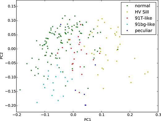
Plot of the first two PCs for the SNe Ia of our sample. The classification is according to Blondin et al. (2012).
Binning and number of spectra. Time is measured in days relative to B-band maximum.
| tmin . | tmax . | Number . |
|---|---|---|
| . | . | of spectra . |
| −12.5 | −10.0 | 90 |
| −10.0 | −7.5 | 165 |
| −7.5 | −5.0 | 218 |
| −5.0 | −2.5 | 233 |
| −2.5 | 0.0 | 256 |
| 0.0 | 2.5 | 258 |
| 2.5 | 5.0 | 231 |
| 5.0 | 7.5 | 177 |
| 7.5 | 10.0 | 170 |
| 10.0 | 12.5 | 160 |
| 12.5 | 15.0 | 101 |
| 15.0 | 17.5 | 95 |
A few typical examples of data we used in our analysis are given in Appendix A.
2.2 The method
In general terms, PCA is a standard statistical tool for data reduction. It reduces the dimensionality of a data set with an intrinsically high number of dimensions, but retaining the meaningful information. PCA is essentially a rotation of the axes of the high-dimensional space representing the data that aligns the first axis to the direction with the largest variance, the first PC. The second PC maximizes the variance, subject to being orthogonal to the first, and so on. Thus, an initially multivariate data set is described by a smaller number of uncorrelated parameters.
Here, we present a brief summary of a variant of the method developed in Sasdelli et al. (2015) and refer for details to our previous work. In order to study systematically the spectral characteristics of different explosion scenarios, we use a method to construct a metric space for SN Ia spectral time series. We use an Expectation Maximization Principal Component Analysis (EMPCA; Roweis 1998; Bailey 2012) on the space of spectral series. The most important idea behind our approach is to study the derivative of the flux over wavelength (∂F(λ)/∂λ) of the spectra instead of the flux (F(λ)) itself. The use of derivative spectroscopy suppresses the variance associated with reddening, uncertainties in the distance and calibration of the flux. Another key ingredient is the use of series of epochs to include the information of spectral evolution (e.g. velocity gradients, Benetti et al. 2005), and not only spectral indicators at maximum. The final step is the use of PLS regression. This is a robust way to find relations between spectra and photometric properties, such as absolute magnitudes and intrinsic colours. The method to construct the metric space and apply PLS regression is detailed in Sasdelli et al. (2015). In this section, we describe again the crucial steps of the method and explain a few incremental improvements.
2.2.1 Derivative spectroscopy
In order to obtain meaningful derivatives of the fluxes the observed spectra have to be smoothed. Here, we apply an improved Savitzky–Golay filter (Savitzky & Golay 1964) for smoothing. A well-known way to improve low band pass filters is to iterate the filtering a number of times (Kaiser & Hamming 1977). The fit of a third-grade polynomial on a window of 1800 km s−1 is iterated five times. With this filtering, we improved the rejection of the noise and at the same time obtained sharper spectral features to be fed into the PCA algorithm.
2.2.2 Spectral series and EMPCA
The input matrix for the analysis is formed by observations (rows) and observables (columns). Every supernova is an individual observation and the derivatives of the fluxes of spectra at different epochs are treated as different observables. The input vectors of this matrix are constructed concatenating spectra at different epochs in the spectral series. The EMPCA code of Bailey (2012) deals automatically with missing epochs and/or wavelength gaps in the data. The derivative analysis frees us from the need of flux calibrated spectra with known distances, and the large number of low noise spectra for nearby SNe allows us to increase the included range of epochs over what was done in Sasdelli et al. (2015). We now include spectra from −12.5 d up to +17.5 d from B maximum. The spectral coverage of CfA supernovae, by number the largest of the sample, is usually limited to below ∼7000 Å. This restricts our current analysis to a spectral range between ∼3500 and ∼7000 Å. This is not a major issue here, since some of the information redward of 7000 Å (mostly in the IR triplet of Ca ii) is also present in the included wavelength range as was shown in Sasdelli et al. (2015). The metric space resulting from PCA has a low dimensionality. The output consists of just five significant components.
The metric space obtained from public data is similar to the one obtained in our previous work on SNf data. Projecting the supernovae on the first three PCs (Figs 1 and 2) shows the groups found in our previous work also (fig. 7 of Sasdelli et al. 2015). Using the first four to five dimensions, the metric space obtained from the public SNe Ia clearly distinguishes the spectroscopic subtypes. Normal SNe Ia are on the top-left side of the cloud of points in Fig. 1, supernovae with a high-velocity photospheric Si ii 6355 Å have a large first component, 1991T-like events have negative third component (Fig. 2). In the public sample we have also fainter supernovae. There is a significant number of 1991bg-like SNe, characterized by fast declining light curves, low luminosity and low temperature of the spectra. At the bottom of Fig. 1, further apart than 1991T-like, there are a number of supernovae called peculiar by Blondin et al. (2012). Many of them are 2002cx-like. This is another class of faint objects characterized by hot spectra and very low line velocities. These faint SNe Ia are absent in the SNf cosmology sample and are not well represented in the publicly available data either.
In Appendix A, we present several examples showing the quality of our PCA reconstruction as well as possible problems for supernovae of various subtypes. We demonstrate that the method works fine even in the case of noisy spectra and/or missing data, provided there is a sufficient number of similar objects in the training set.
2.2.3 PLS regression
The final and crucial ingredient in our approach is a PLS regression (Wold 1982; Wold et al. 1984). It is also known as Projection to Latent Structures, the latter name describing better the aim of the technique. With this tool, we find the empirical relations between the spectral properties encoded in the PCA space and photometric properties, such as Δm15(B), the intrinsic part of the B − V colour or the absolute B magnitude. The underlying assumption is that the intrinsic colour [absolute B magnitude or Δm15(B)] is a function of the spectral properties of the supernova and can be predicted from them.
With this metric space, we can check if different explosion scenarios are consistent with empirical relationships between spectral and photometric properties that hold for SNe Ia and thereby analyse potential advantages or shortcomings of the various classes of models.
3 EXPLOSION SCENARIOS
It is widely accepted that SNe Ia are the result of the thermonuclear explosion of a carbon–oxygen white dwarf triggered by the interaction with a companion star. But beyond this very little is known with certainty. In this section, we briefly review the presently favoured scenarios (see also Hillebrandt et al. 2013 for a recent review).
3.1 Delayed detonations
The delayed detonation model (Khokhlov 1991) is one of the most studied scenarios as an explanation for SNe Ia. This explosion mechanism is usually proposed for single-degenerate systems where a carbon–oxygen white dwarf explodes close to the Chandrasekhar mass MChan (∼1.4 M⊙) after accreting mass from a non-degenerate companion, presumably through Roche lobe overflow. The matter steadily burns to carbon and oxygen on the surface of the white dwarf increasing its mass until the density at the centre is sufficient for the ignition of nuclear burning and for a combustion wave to form.
In this class of models, it is assumed that in the beginning burning proceeds with a flame speed lower than the speed of sound (deflagration) and incinerates the interior of the star. This phase allows for the white dwarf to expand and decrease the density of the unburned material, a necessary ingredient for the synthesis of intermediate mass elements (IMEs). It is further assumed that in a next step a transition from a deflagration to a detonation takes place somewhere in the star with a burning velocity now larger than the speed of sound. Whether or not this happens in reality is heavily disputed (Röpke 2007; Woosley 2007; Aspden, Bell & Woosley 2010; Schmidt et al. 2010; Poludnenko, Gardiner & Oran 2011; Charignon & Chièze 2013), but it cures several of the problems of pure-deflagration models (see Section 3.2), i.e. these models can be brighter and have less unburned carbon and oxygen at low velocity. In fact, after the transition the detonation front quickly burns most of the remaining fuel, partially to 56Ni and partially to IMEs (Hoeflich & Khokhlov 1996; Mazzali et al. 2007; Kasen, Röpke & Woosley 2009; Blondin et al. 2011, 2013; Sim et al. 2013). It is this property of the delayed detonation models that brings Chandrasekhar-mass explosions closer to the observed light curves and spectra of normal SN Ia than pure-deflagration models.
3.2 Pure deflagrations
Historically, pure deflagrations of MChan carbon–oxygen white dwarfs such as the W7 model (Nomoto, Thielemann & Yokoi 1984) have been favoured as an explanation for normal SNe Ia. The W7 model is a 1D deflagration with a parametrized flame speed, assumed to be proportional to the distance from the centre of the star. However, in this model the burning proceeds faster than what happens in recent 3D deflagrations (Röpke et al. 2007; Fink et al. 2014; Long et al. 2014; Malone et al. 2014) leading to nuclear burning comparable to the delayed detonation models. W7 is generally in reasonable agreement with normal SNe Ia, although at later times it seems to have a core structure different from the prototypical normal SN 1994D (Lentz et al. 2001).
In recent deflagration models, the initial conditions are the same as in the delayed detonations, but the (unproven) deflagration to detonation transition (see Section 3.1) does not happen. Consequently, for equivalent initial conditions, the burning is less complete than in the corresponding delayed detonation models. The production of 56Ni is more limited and this limits the maximum possible luminosity of the scenario (Röpke et al. 2007). Hence, this mechanism cannot be an explanation for the brightest SNe Ia but may explain some faint peculiar subtypes of SNe Ia (Jordan et al. 2012; Kromer et al. 2013a, 2015; Stritzinger et al. 2015).
3.3 Sub-Chandrasekhar-mass detonations
The Sub-Chandrasekhar-mass models investigated here, i.e. exploding white dwarfs with a mass lower than MChan, are the result of detonations ignited near the centre of the white dwarf. The rates of this progenitor channel are easier to explain using binary population synthesis simulations (Ruiter et al. 2011) than the single-degenerate scenario. In contrast to the MChan case, for these stars the density at the centre is not high enough to self-ignite carbon and oxygen but a trigger is needed. A possible mechanism is the so-called double-detonation (Livne 1990). A layer of helium-rich material on the surface of the white dwarf may detonate first, for example after it was accreted from a companion (He-)star or during a merger with the companion. The He-detonation will engulf the white dwarf sending shock waves inward which will converge close to the centre. Numerical simulations have shown (Fink, Hillebrandt & Röpke 2007; Fink et al. 2010; Moll & Woosley 2013) that in the converging shocks the temperature increases sufficiently to trigger a secondary detonation in the C+O fuel. Burning at the lower density of the sub-MChan white dwarf (as compared to the MChan case) produces naturally a large amount of IME (that are seen in the ejecta), and the mass of the initial white dwarf (setting its density) is an excellent parameter to drive the mass of 56Ni and reproduce the variance in luminosity observed in SNe Ia (Sim et al. 2010). We note, however, that the models of Sim et al. (2010) are explosions of bare CO-cores which may be more generic but less realistic than specific double detonations including the He shell.
3.4 Double-degenerate mergers
A scenario different from the previous ones is the merger of two sub-MChan C+O white dwarfs (Iben & Tutukov 1984; Webbink 1984). The comparison of recent population synthesis simulations (e.g. Ruiter, Belczynski & Fryer 2009; Toonen, Nelemans & Portegies Zwart 2012) with the observed rates favours this scenario over single-degenerate progenitors. The orbit of such binary systems slowly decays through gravitational wave emission until the two stars merge. If this happens on a time-scale shorter than the Hubble time, the binary may be a candidate for an SN Ia. The process of merging may trigger an explosion in the primary through the double-detonation mechanism explained in the previous section (Pakmor et al. 2013). If an adequate He layer is not present, the rapid accretion due to tidal interaction may form a hotspot on the primary with a high enough density to trigger the detonation of carbon there (Pakmor et al. 2012; Moll et al. 2014).
If, however, the burning does not start promptly, the secondary will be disrupted over a few orbits and will be accreted on to the primary on a secular time-scale. If during this process the mass of the primary gets close to MChan either an explosion is triggered at the centre or the white dwarf may collapse to a neutron star (Miyaji et al. 1980; Saio & Nomoto 1985). In case of an explosion, this scenario might resemble fast rotating MChan models.
Here, we will investigate models only in which the explosion is triggered promptly. As in the case of sub-MChan detonations, the mass of 56Ni is largely determined by the mass of the primary white dwarf. The mass of the secondary and the viewing angle could be additional parameters explaining the diversity within SNe Ia. Alternatively, if the two white dwarfs have comparable masses both stars are disrupted during the interaction. In the case of two 0.9 M⊙ white dwarfs, it was found that the low central density leads to little 56Ni production and to a significantly lower luminosity compared to mergers with a similar but unequal and larger progenitor masses. Therefore, it was suggested as a scenario for the SN 1991bg-like subluminous supernovae.
4 THE MODELS IN PCA SPACE
At our disposal, we have a series of 3D numerical simulations for all classes of models discussed in the previous section, to be compared with the observations. The models that we used and the original papers are summarized in Table 2. In this work, we focus on the angle averaged spectra and light curves from these models. It will be the topic of a future paper to use the lines of sight individually. At first we will check the general consistency of the spectra with observed SNe Ia. To do so, we will use only the first part of our analysis that is the PCA space. The position of the models in the first dimensions of the PCA space gives interesting clues about the spectral behaviour of the models. Figs 3 and 4 show where models lie in the projections on the first three PCs. These are the most significant ones. Normalizing to the first component, the second component has ∼45 per cent of the variance of the first. The third has ∼43 per cent. The fourth component has only ∼25 per cent of the variance of the first component. The first five PCs cover more than 90 per cent of the total variance in the data. As example, the spectrum of the W7 model at B-band maximum and its reconstruction from the PCA space by means of five PCs is shown in Fig. 5. More examples are shown and discussed in Appendix B.
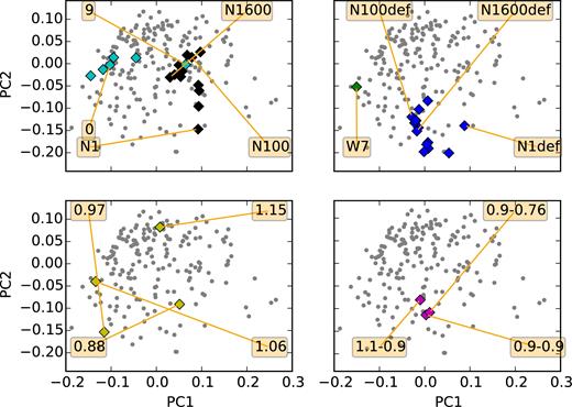
The first two PCs of the data (grey dots) with the projections of the analysed models overplotted. Most of the models are well inside the PC space determined by the data in the most important components. Model series are characterized by chains of points in a multidimensional space. The top-right diagram shows the position of W7 on the low-luminous edge of normal SN Ia and the 3D deflagrations populating the space of the faint 02cx-like SNe. The top-left diagram shows the series delayed detonation models with a variable number of ignition spots (black) and models with the composition of N100 and a progressively larger degree of mixing (0 to 9, cyan). The bottom-left diagram shows the sub-Chandra detonations with different initial masses (yellow). The bottom-right panel shows three merger models with different initial masses (magenta).
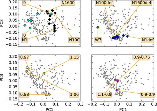
The first and the third PCs of the data and of the models overplotted. The panels are the analogous of Fig. 3. deflagrations (top-right), delayed detonation (top-left), sub-Chandra (bottom-left), mergers (bottom-right).
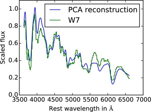
The figure shows the spectrum of the W7 model at B maximum and the corresponding reconstruction using PCA.
| Model names . | Hydro paper . | Rad transport paper . |
|---|---|---|
| Delayed detonations . | . | . |
| N1,[...],N1600 | Seitenzahl et al. (2013) | Sim et al. (2013) |
| Pure deflagrations | ||
| N1def,[...],N1600def | Fink et al. (2014) | Fink et al. (2014) |
| W7 | Nomoto et al. (1984) | Kromer & Sim (2009) |
| Sub-Chandrasekhar mass detonations | ||
| 0.88, 0.97, 1.06, 1.15 | Sim et al. (2010) | Sim et al. (2010) |
| Double-degenerate mergers | ||
| 0.9–0.9 | Pakmor et al. (2010) | Pakmor et al. (2010) |
| 1.1–0.9 | Pakmor et al. (2012) | Pakmor et al. (2012) |
| 0.9–0.76 | Kromer et al. (2013b) | Kromer et al. (2013b) |
The model classes are characterized by the variation of a single input parameter (the white dwarf's mass in case of sub-MChan models, the number of ignition spots in case of delayed detonations and deflagrations, and the masses of the two white dwarfs in case of mergers). They show up in our PC space as chains of points describing curves in the 5D space. Along these curves, the input parameter varies continuously leading to continuous variations of the spectral properties. Most of these models lie well within the space of observed SNe Ia and cover a fair fraction of their diversity.
More specifically, we use sub-MChan detonations (Sim et al. 2010) in the range of 0.97–1.15 M⊙. These models draw a curved line running clockwise when projected on the first two dimensions (Fig. 3, bottom-left panel) that connects faint 1991bg-like supernovae with normal SNe Ia. The faint model with 0.88 M⊙ marks the beginning of this line, and it is quite far away from most normal SNe Ia. Its next neighbours are faint 1991bg-like and 2002cx-like supernovae. This is not unexpected and is a confirmation of the general behaviour of the sub-MChan models (Sim et al. 2010).
Our delayed-detonation models (Seitenzahl et al. 2013; Sim et al. 2013) lie in a completely different part of the PC space (Fig. 3, upper-left panel). In these delayed-detonation models, the initial condition that is varied is the number of ignition spots (N). This affects the strength of the deflagration phase. During the deflagration phase the rate of nuclear burning is proportional to the surface area of the burning front. A small number of ignition spots means that burning is less complete when the conditions for the transition to a detonation are met. This in turn implies less pre-expansion of the white dwarf and a more complete burning in the detonation phase with more 56Ni being produced. In the first two components the models draw a line that goes from normal SNe Ia with high photospheric line velocities (N1600, 1600 ignition spots) down to hot and bright SNe Ia (N1, one ignition spot). This behaviour is also in line with what is expected from this class of models (Sim et al. 2013).
Klauser (B.A. Thesis, LMU) created a series of 1D models using a spherical average of N100 (Seitenzahl et al. 2013) as a starting point. First, he constructed a completely stratified version of the N100 model preserving the total masses of the most important elements and the density profile. Iron group elements (IGEs) different from 56Ni are represented by stable Fe. Then, starting from this model he introduced progressively more mixing by convolving the abundances with a Gaussian window. The density profile and the total masses of the different elements are kept constant. This makes the model consistent with the total energy output. Also, inspired by the results from the ‘abundance tomography’ technique (e.g. Mazzali et al. 2015), the 56Ni is placed outside of the stable Fe. The models add a component clearly orthogonal to the trend of the delayed detonation models (Figs 3 and 4). From now on we call these models ‘artificially mixed N100’. This finding shows that a mechanism that suppresses mixing in some cases can potentially explain part of the remaining diversity of SNe Ia spectra not matched by varying the number of ignition spots.
The deflagration models from Fink et al. (2014) stay in the part of the diagram that belongs to the faint 02cx-like SNe (Fig. 3, top-right panel). The prototypical parametrized deflagration W7 model is closer to the bulk of the spectroscopically normal SNe Ia.
The two merger models with progenitors of different mass (Pakmor et al. 2012; Kromer et al. 2013b) are close to the centre of the distribution. The faintest merger of white dwarfs of equal masses (Pakmor et al. 2010) is more separated from the others and closer to 91bg-likes (Fig. 4, bottom-right panel).
In Appendix B, we show how the reconstructed model spectra compare with their original counterparts and how they compare with the nearest observed neighbours in PCA space. We find that the agreement is quite good in general, but becomes poor in cases where the synthetic spectra are very different from the bulk of the data used to construct the PCA space. However, this was expected and has to be taken into consideration when comparing models with data. Also, one has to keep in mind that plots like Figs 3 and 4 are projections only and that the ‘real’ distance in PCA space of a model to its observed neighbours may be larger than it appears to be.
In the literature, it is extensively discussed that in order to have a good scenario for SNe Ia, the luminosity range, the luminosity-decline rate relation and the rise time have to agree. But it is also important to have consistency between spectral and photometric properties. This will be investigated in the following section.
5 PROJECTING SPECTRAL PROPERTIES INTO PHOTOMETRIC PROPERTIES BY PLS
In this section, we check the consistency between spectral series and a set of well-studied photometric properties with the aid of PLS regression. The effect of dust extinction on the space of photometric properties is marginalized by rejecting highly extinguished SNe.
5.1 Δm15(B)
The first relation against which we test the models is the correlation between spectral properties and Δm15(B). In particular, we study the empirical relation that we found in Sasdelli et al. (2015). This is analogous to the relation between the ratio of the depth of the Si ii 5972 Å and the Si ii 6355 Å lines and Δm15(B) (Nugent et al. 1995), but studied with the systematic approach of the PLS. We stress that the relation explored in this section is not equivalent to the Phillips relation and it is an additional constraint on the models. It is a relation between global spectral properties [predicted Δm15(B)] and light-curve decline [observed Δm15(B)].
In Fig. 6, we show the correlation between Δm15(B) and the direction in the PCA space that correlates with it. It is found by PLS and by using public data only. This direction is close to the direction that predicts the equivalent width of Si ii 5972 Å (Sasdelli et al. 2015, fig. 12). The projections of models representative for the different scenarios are overplotted.

The grey dots show the relation of Δm15(B) versus the predictions obtained by using PLS on the PCA space of spectra for observed SNe Ia. The models are deflagrations (top-right), delayed detonation (black) and modified-mixing models (cyan) (top-left), sub-Chandra (bottom-left), mergers (bottom-right). Errors on the predictions come from k-folding (Sasdelli et al. 2015) and are smaller than the size of the diamonds. The variance on the observed Δm15(B) of mergers and delayed-detonation models comes from the variability due to line-of-sight effects.
In the interval between 0.97 and 1.15 M⊙ the sub-Chandrasekhar-mass detonation models reproduce the fast decline part of the relation remarkably well (yellow diamonds in Fig. 6). This is not too surprising since it was shown in Sim et al. (2010) that they follow the Phillips relation. However, they do not reach the slow decline part of the relation.
In principle, the parameter space of the merger model is large and with the three models available to date we can just begin to explore it. The brightest merger (1.1 and 0.9 M⊙) is clearly below the empirical relation, particularly for some line of sights (indicated by the error bars). This means that, for the given spectral properties of the model, its light-curve evolution is too slow (Pakmor et al. 2012; Röpke et al. 2012). In turn, this implies that the opacity of the model is too large which slows down the evolution of the light curve. A likely explanation is that the total mass is too large to reproduce the bulk of normal SNe Ia. This interpretation is confirmed by the qualitatively similar merger model (0.9 and 0.76 M⊙) which matches the relationship much better, however, this model cannot be considered a good match for normal SNe Ia from a luminosity or spectroscopic point of view (see section 5.3). The equal-mass merger (0.9 and 0.9 M⊙) lies also on the relation.
W7, the classical 1D deflagration model from Nomoto et al. (1984), that is a good match for spectroscopically normal SNe Ia at early epochs, lies well on the relation. However, the more realistic deflagration models do not match spectroscopically with the bulk of SNe Ia (see Section 4). This is why the PLS regression, that works well in predicting the Δm15(B) for the bulk of SNe Ia, returns a value close to the average Δm15(B) for these objects. A richer training sample including more faint objects is necessary to study such a scenario with PLS.
The 3D delayed detonation models from Seitenzahl et al. (2013) and Sim et al. (2013) cluster in a single area of the empirical relation, but do not show its observed trend. Since in the models the number of ignition spots was used to parametrize the strength of the initial deflagration this means that at least one more parameter is needed to reproduce the relation within this class of models. Moreover, models with low or moderate deflagration strength (N lower than about 300) are within the observed range.
Finally, the models plotted as cyan diamonds in Fig. 6 are the artificially mixed N100 models Klauser (B.A. Thesis, LMU). In contrast to the other delayed-detonation models, they do follow the empirical relation and models with a low degree of mixing have larger predicted and observed Δm15(B). This may indicate that a mechanism that allows for more stratified ejecta may be needed in order to reproduce the observed correlation between Δm15(B) and spectral properties with this class of models. Rayleigh–Taylor instabilities in the equatorial plane are suppressed by rotation. Hence, rotation is a possible mechanism that may help in suppressing mixing. Pfannes et al. (2010a) and Pfannes, Niemeyer & Schmidt (2010b) studied explosions of differentially rotating white dwarfs and concluded that they cannot be a good explanation for normal SNe Ia. However, systematic studies of rigidly rotating white dwarfs are still missing.
5.2 B − V colours
Next, we study the consistency of the B − V colour of the models at B-band maximum with the observations. The relation between colour and spectral properties is similar to the relation between colour and velocity of Si ii 6355 Å (Foley & Kasen 2011). Once again, our approach allows for a systematic study of this property and it allows us to use all the information present in the spectra at different epochs, and not only the behaviour of the spectra at B-band maximum.
An important remark here is that in principle our analysis is valid for all SNe Ia. This includes spectroscopically normal SNe Ia, 1991T-likes, those with broad lines (Branch et al. 2006), and others. But it is not possible to study their colour without enough photometric data. In particular the 1991bg-like and the 2002cx-like events present in the sample, although they cluster nicely in different parts of the PCA space (see Section 4), do not have well enough measured photometry to study their colours with the PLS analysis.
To quantify for which SNe we can reliably predict the colours we check if a given SN has neighbours which are selected to have negligible reddening by the PLS algorithm. In Fig. 7, the SNe are coloured in blue if they are selected by the PLS algorithm and have negligible reddening. They are coloured in red if they are not selected as unreddened by the PLS algorithm, but have close neighbours that are unreddened. This means that the colour excess is likely due to reddening. The SNe that do not have a neighbour selected as unreddened are coloured in yellow. They are 1991bg-like and 2002cx-like. For those we cannot predict their colour or luminosity using PLS.
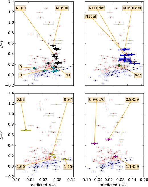
The B − V colour at B-max (without reddening corrections) and the B − V colour predicted from spectral properties using PCA and PLS. The SNe are represented by dots. SNe with small reddening are in blue, the SNe with significant reddening are in red. Errors on the predicted colours come from k-folding (Sasdelli et al. 2015) on the PLS regression analysis. Only the blue points are representative of the intrinsic SN properties, the relation is the blue dashed line. SNe in yellow belong to a part of the space with not enough photometric data. For them the predicted colour is not reliable. The models are represented by diamonds. The models are W7 and 3D deflagrations (top-right), delayed-detonation and modified-mixing models (top-left), sub-Chandra (bottom-left), mergers (bottom-right).
With this in mind, the empirical relation between intrinsic colour and spectral properties holds for the bulk of SNe Ia, but not for most peculiar SNe. Therefore, the relation has to hold for models proposed to describe the bulk of SNe Ia but not for rare objects. Of course, by construction, the models are not reddened. Only models that fit in the relation defined by the SNe coloured in blue can explain the bulk of SNe Ia. Ideally, a perfect scenario for normal SNe Ia has to lie in the strip populated by blue dots in Figs 7 and 8. Some of the models that are off this relation can be a good explanation for some of the peculiar SNe coloured in yellow. For these SNe, the PLS-predicted quantity is just a linear extrapolation of what is valid for normal SNe. Until a significantly larger sample is available, these peculiar SNe need to be studied on a case-by-case basis.
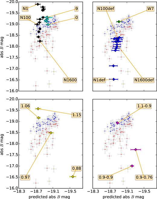
The absolute B-band maximum without reddening corrections and the predicted B-max using PCA and PLS. The models are W7 (top-right, green), 3D deflagrations (top-right, blue), delayed-detonation (black) and modified-mixing models (cyan) (top-left), sub-Chandra (bottom-left), mergers (bottom-right). Errors on the predictors come from k-folding on the PLS regression analysis (Sasdelli et al. 2015). (See Fig. 7.) The models that are far away from the blue strip cannot explain normal SNe Ia. However, some can be good candidates for some peculiar SNe Ia (e.g. SNe marked in yellow).
Many of the models suffer from being too red compared to the observations (Fig. 7). This systematic issue is well known (e.g Sim et al. 2013) and it may be due to approximations in the radiation transport code or shortcomings in the hydrodynamic modelling. Here, we focus on the trend between intrinsic colour and spectral properties that holds for the majority of observed SNe Ia, but does not seem to be clearly reproduced by any of the investigated explosion scenarios for which more than one realization exists.
The intrinsic colour of SNe Ia correlates with the velocity of the main Si ii line (Foley & Kasen 2011). SNe Ia with a higher velocity have redder colour. Consequently, the delayed detonation models, well known for having high photospheric velocities (Sim et al. 2013), place themselves in the right side of the diagram in Fig. 7 (top-left panel), where the intrinsic colour is larger than ∼0.1. However, most of these models are still too red. For example, N100, a delayed detonation model proposed as explanation for normal SNe Ia, is too red by ∼0.3 mag. It is interesting to note that models with the same composition, but with an enforced stratification, reproduce the trend of the observed relation fairly well. The crucial difference in obtaining the right colour can be due to the stratification of the inner parts of the ejecta. These modified models have stable iron at the centre and 56Ni around it. This changes the way the light is reprocessed and makes the colour less red. We also note that the 2D delayed detonation models of Kasen et al. (2009) are systematically bluer than our models. However, it is unclear to which extent this is due to the reduced dimensionality of the models differences in the radiative transfer or nucleosynthesis post-processing.
Both the sub-MChan models and the delayed-detonation models show a trend that is opposite to the one observed for normal SNe Ia. Brighter models have IME at higher velocities. This trend seems to be a robust characteristic of these scenarios. For the sub-MChan models, more massive progenitors will naturally have higher kinetic energies and ejecta opaque up to higher velocities. Also, the IME layer moves at higher velocities because more IGEs are produced near the centre. At the same time, more massive and brighter models, within the range of luminosities of typical SNe Ia, are going to be hotter and thus bluer. Among normal SNe Ia, those with lower photospheric velocities can have both, greater or lower luminosity. For the delayed detonations, more complete burning releases more energy. If the binding energy is the same, the kinetic energy will be larger.
As previously discussed, there are not enough data available to study the colour of 1991bg-like SNe with PLS regression. However, peculiar 1991bg-like supernovae are known to have low photospheric velocities and to be intrinsically redder than normal ones (Turatto et al. 1996). For them, the sub-MChan models with a low mass may be a viable scenario.
The colour of the brightest merger model considered is quite right, just a bit too red (Fig. 7, bottom-right panel), and this could be due to issues in the radiation transport and not in the scenario itself. We need merger models with initial conditions similar to the brightest merger to check if this scenario reproduces the trend observed for normal SNe Ia. The merger models with lower masses are too far away from the properties of normal SNe Ia to be used to extrapolate such a relation.
5.3 B magnitudes
In order to study the relation between spectral properties and absolute magnitudes, we need to have an estimate of the absolute magnitude, independent of the assumption of a width–luminosity relation of the light curves. Assuming a Hubble constant of 70 km s−1 Mpc−1, we use the redshift as a measure of distance. The error of the absolute magnitude is then the error on the observed magnitude with an error due to the peculiar motions of the galaxies added in quadrature. We do not attempt to perform any reddening correction. Similarly to the case of the colours, we cannot study the faintest SNe Ia with statistical methods since we do not have enough 1991bg-like and 2002cx-like supernovae in the smooth Hubble flow.
In Fig. 8, sub-MChan models with initial masses between 0.97 and 1.15 M⊙ bridge the correct range of luminosities of the bulk of SNe Ia. However, they are orthogonal to the empirical relation between luminosity and spectral properties. Among the brightest representatives of the SN Ia population are 1991T-like SNe. They are fairly common and are characterized by spectra with high temperature and somewhat lower than normal photospheric velocities. This is in contrast to what the sub-MChan models predict. SNe with ‘normal’ luminosities show a diverse range of photospheric velocities that is correlated with colour, but not with luminosity. To explain the variability shown in the spectra a parameter other than the mass at explosion is needed in the sub-MChan scenario. This parameter needs to decrease the 56Ni mass of the ejecta to slow down the time evolution without changing the total mass.
Fig. 8 shows that delayed-detonation models can also explain the appropriate range of luminosities easily but, like the sub-MChan models they are mostly orthogonal to the observed relation. The behaviour of models with limited mixing suggests that a mechanism to suppress mixing in the ejecta can possibly bring the delayed-detonation models into closer agreement with the observations. Models with high stratification in the ejecta go towards the right side of the diagram. In order to explain the bright SNe Ia, a high stratification of the ejecta seems to be necessary. Significant rotation of the progenitor may be a possibility to suppress mixing and to produce more stratified ejecta.
The W7 model is placed close to the relation. The modern 3D deflagration models, on the other hand, are significantly fainter than the bulk of SN Ia, and cannot be used to explain them. Their luminosity, however, is compatible with some of the faint classes such as 02cx-like SNe.
The brightest merger model lies nicely on the relation observed for the bulk of SNe Ia. The lower mass mergers are too faint for such a relation, and they cannot be an explanation for it. However, they can explain fainter and rarer objects. To assess if the merger scenario is a viable explanation for the majority of SN Ia, one has to explore the parameter space close to the bright 1.1 and 0.9 M⊙ merger model to see if the relation holds. The faintest merger models cannot be a good explanation for the normal SNe Ia. Their B-band luminosity, as predicted from their spectral properties, would be far too high (see Fig. 8). The predicted B mag is just a projection of the PCA space, and it is a good prediction for the B mag for the bulk of SNe Ia only. The fact that these models are off such a relation does not mean that they do not provide an explanation for some peculiar objects (e.g. Kromer et al. 2013b).
6 CONCLUSIONS
Sasdelli et al. (2015) studied the empirical relations between the small wavelength spectroscopic properties of SNe Ia and photometry. In this work, we test a number of models for these relations. Our tool allows a systematic comparison between synthetic and real SN Ia spectra. We use PCA on time series of observed SN Ia spectra to reduce the dimensionality of the data. Projecting the synthetic spectral series of a particular model in the PC space revealed its counterparts among the real supernovae by an analysis of its neighbours. Moreover, the relations discovered by PLS are strong tests that the models have to pass. Given the challenge of performing a coherent statistical comparison between synthetic and real spectra, our method is particularly efficient in characterizing large sets of models built from different explosion scenarios. It is able to provide important insights regarding the global properties of each explosion mechanism in order to favour or disfavour them. Such a global analysis is also expected to be more robust against systematics in the models (for example due to approximations in the radiation transport) than comparing them individually on a case-by-case basis with real SNe.
Much of the known behaviour of the models is recovered in our work. For example, the pure deflagration models can be an explanation for faint SNe Ia (Jordan et al. 2012; Kromer et al. 2013a, 2015; Stritzinger et al. 2015). Similarly, also the merger models with equal initial masses (0.9–0.9 M⊙) are a good candidate for faint SNe Ia (Pakmor et al. 2010). The sub-Chandrasekhar-mass detonations and the delayed detonations are the best candidates for normal SN Ia (Sim et al. 2010; Ruiter et al. 2011). However our technique shows that they both have shortcomings that need to be addressed. The number of merger models studied is very limited, and only one is a good candidate for normal SNe Ia. So it is hard to put strong constraints on this scenario.
In addition to what was known before, our tool offers very stringent tests for those models that are candidates for the bulk of SNe Ia, thanks to the abundant observational data. We find that the relations between spectroscopic and photometric properties predicted by the sub-MChan models do not follow the relations that are valid for the bulk of SN Ia. On the other hand, sub-MChan models with masses lower than 0.97 M⊙ are very good candidates for the faint SN Ia, where such relations are reproduced. Some of the shortcomings of the delayed detonation models as an explanation for the bulk of SNe Ia may be cured by a mechanism that reduces mixing in the brightest models. We propose rotation as a possibility to achieve this result. A merger model with masses (1.1–0.9 M⊙), proposed as an explanation for the bulk of SNe Ia, evolves somewhat too slowly in relation to its spectral properties. This suggests an ejecta mass that is somewhat too high. On the other hand, it is positioned quite well in the diagrams that show luminosity or colour. An investigation of more merger models is necessary to reach definitive conclusions for this scenario.
Once a large enough library of synthetic spectra becomes available, an alternative PC space may be constructed directly from the models. Projecting the observed SNe to such a model PC space, will provide a critical cross check between the real and synthetic metric spaces. In addition, our approach is well suited to systematically assess viewing-angle effects in multidimensional explosion models, which is very difficult on an individual basis. Both of these aspects will be addressed in future work.
The authors gratefully acknowledge the Gauss Centre for Supercomputing (GCS) for providing computing time through the John von Neumann Institute for Computing (NIC) on the GCS share of the supercomputer JUQUEEN (Stephan & Docter 2015) at Jülich Supercomputing Centre (JSC). GCS is the alliance of the three national supercomputing centres HLRS (Universität Stuttgart), JSC (Forschungszentrum Jülich) and LRZ (Bayerische Akademie der Wissenschaften), funded by the German Federal Ministry of Education and Research (BMBF) and the German State Ministries for Research of Baden-Württemberg (MWK), Bayern (StMWFK) and Nordrhein-Westfalen (MIWF). The work of FKR is supported by the ARCHES prize of the German Ministry of Education and Research (BMBF) and by the DAAD/Go8 German-Australian exchange programme for travel support. The work of FKR and RP is supported by the Klaus Tschira Foundation. EEOI is partially supported by the Brazilian agency CAPES (grant number 9229-13-2). IRS was supported by the Australian Research Council Laureate Grant FL0992131. RP acknowledges support by the European Research Council under ERC-StG grant EXAGAL-308037. WH acknowledge support by project TRR 33 The Dark Universe of the German Research Foundation (DFG) and the Excellence Cluster ‘Origin and Structure of the Universe’ at the Technische Universität München.
REFERENCES
APPENDIX A: PCA RECONSTRUCTION OF OBSERVED SUPERNOVAE
In this Appendix, we show spectra of several supernovae from our sample together with their PCA reconstruction. To demonstrate the power (and potential weaknesses) of the method, we have chosen examples from the various groups in Figs 1 and 2, i.e. ‘normal’, ‘HV SiII’, ‘91T-like’, ‘91bg-like’ and ‘peculiar’, as well as some with good or poor time coverage, and some with good or noisy data. In all figures that follow the logarithm of flux over wavelength is plotted for the wavelength range used in our EMPCA. Each spectrum is labelled with the time measured from B-band maximum, and time is progressing from bottom to top. Observed spectra are in green and reconstructed spectra are in blue. The reconstruction is done with the first five principle components. Note that in our analysis all epochs are binned. The bins are 2.5 d wide. The curves in the figures are labelled with the mid-points of each bin.
We start by discussing a few spectroscopically normal SNe Ia. Fig. A1 shows SN 2000dm in UGC 11198 discovered by the Katzman Automated Imaging Telescope (KAIT) Lick Observatory Supernova Search team, for which we have three spectra only. Nevertheless, the reconstructed spectra agree reasonably well with their observed counterparts at all epochs. In more general terms, some noise or some missing epochs are not a problem if the epoch coverage spans the range of the analysis.
The second example, SN 2002jg in NGC 7253, also discovered by KAIT, is another normal SN Ia, but with more noisy data. Fig. A2 shows the four observed spectra and their reconstruction. The fit is not affected by the data quality. However, it can be seen that the colour of the reconstructed spectra is slightly too blue at all epochs, although all spectral features are well reproduced. Such a slight mismatch of colours is seen in several of our reconstructed spectra and is caused by the fact that our analysis is based on the derivatives of the logarithm of the spectra making the predicted colours somewhat uncertain. In addition, reddening does not significantly affect the PCA space. This means that the colour might be poorly reproduced when there is extinction. Since, however, the comparison of models with data is done by means of derivative spectroscopy this shortcoming is not a major problem. The third example, SN 2004as, shown in Fig. A3, is an extreme case in this respect. Here, the reconstructed spectra are too red. However, as before, individual line shapes agree quite well at all epochs. In total, we had 16 spectra in this case.
Next, we discuss subluminous 91bg-like supernovae. Since there are fewer members of this group in our training set, we expect that typically the reconstructed spectra may not fit their observed counterparts as well as they did for the normal ones, and the results confirm this expectation. Fig. A4 shows spectra of the well-observed 91bg-like supernova SN 1999by for which we have a total of 22 spectra. Although the main features are reproduced, the overall fit is not too good. A significantly better reconstruction is found for SN 2002dl (Fig. A5) for which (again with slightly incorrect colours) the fit is very good although the data are rather noisy and we had four spectra only. SN 2002dl is a less ‘extreme’ 91bg-like and this is why it is easier to reproduce. All in all, however, most spectral features of 91bg-like SNe Ia are reasonably well reproduced and some of the shortcomings are not unexpected.
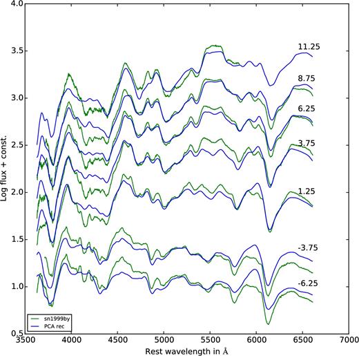
Observed spectra of SN 1999by (in green) with the reconstructed spectra (in blue) overplotted. The data are mostly from Blondin et al. (2012).
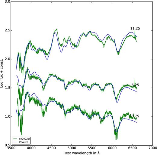
Observed spectra of SN 2002dl (in green) with the reconstructed spectra (in blue) overplotted. The data are from Blondin et al. (2012).
This also holds for 91T-like events, as shown in Figs A6 and A7. For the well observed (16 spectra) SN 1998es in NGC 632, a typical member of this group, besides again a slight mismatch of colour, the reconstruction is good, and it is almost perfect for the late epochs, and the same holds for SN 1999gp (six spectra).
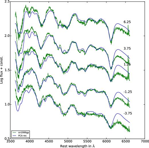
Observed spectra of SN 1999gp (in green) with the reconstructed spectra (in blue) overplotted. The data are from Blondin et al. (2012).
SN 2004ef (21 spectra) and SN 2007le (32 spectra), shown in Figs A8 and A9, are members of the group of supernovae with high photospheric Si ii velocities. They populate a rather large part of the PCA space, indicating significant spectroscopic diversity. Given this fact, the reconstruction works surprisingly well. Again, we find some colour mismatch around maximum light, but otherwise the fits are good in both cases. Note that even spectra with incomplete waveband coverage (as for SN 2007le) are reconstructed rather well.
Finally, we show the reconstruction for SN 2006gz (24 spectra), a peculiar, very luminous carbon-rich supernova, considered to be the prototype of so-called super-Chandrasekhar mass explosions (Fig. A10). As in the cases of 91bg-like and 91T-like supernovae, there are very few members in the training set. Nevertheless, the reconstruction works surprisingly well, especially after peak.
In conclusion, the PCA reconstruction of multi-epoch spectra of SNe Ia works reasonably fine even in cases where the limited number of objects in our training set might have indicated a problem. Also the data quality is not an issue and is taken care of by the method. Therefore, we are confident that we can use the metric space constructed for a comparison with synthetic spectra of models.
APPENDIX B: PCA RECONSTRUCTION OF MODEL SPECTRA AND THEIR COMPARISON WITH REAL SUPERNOVAE
In this Appendix, we show spectra of several of the models used in this paper and compare them with their PCA reconstruction. Such a comparison is necessary since the model spectra are not part of the training set and, therefore, it is not obvious that the reconstructed synthetic spectra do resemble the ‘original’ ones, in particular given the fact that our PCA is based on the derivatives of the spectra. We will do the comparison for one or two typical realizations of each class of models discussed in the main text. As in Appendix A, in all figures the logarithm of flux over wavelength is plotted, and each spectrum is labelled with the time relative to B-band maximum. Time is progressing from bottom to top. Computed model spectra are in green and their reconstructed counterparts are in blue. All model spectra are viewing angle averaged. Note that we plot the observed spectra rather than their PCA reconstruction which makes the comparison even more demanding. As in Appendix A, the epochs are binned and we use five PCs for the reconstruction.
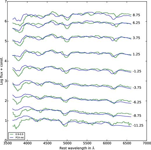
We start with the violent merger models. Fig. B1 shows the spectra predicted for the merger of a 1.1 M⊙ with a 0.9 M⊙ white dwarf. This model was used for a comparison with the normal SN 2011fe by Röpke et al. (2012). The agreement between computed and reconstructed spectra is good for early epochs, but gets worse at late times where also the colour offset is more pronounced. The second merger model we present is for two equal mass (0.9 M⊙) white dwarfs, a model that is known to show similarities with 91bg-like events (Fig. B2) and has been used in this context by Pakmor et al. (2010). Here, the reconstructions are never really good, getting worse for the later spectra. The quality of the reconstruction of 91bg-like is not as good as other more populated subtypes of SNe. This is the likely reason for this discrepancy. Note that also the quality of the reproduction of observed 91bg-like supernovae was not great (see Appendix A).
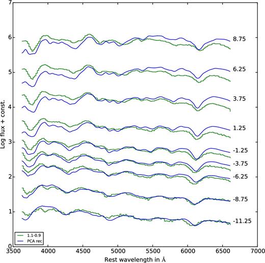
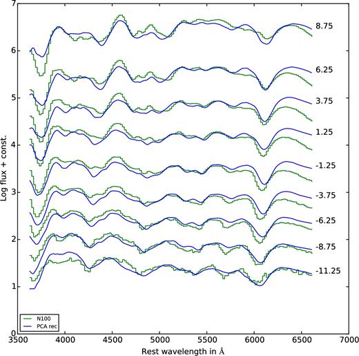
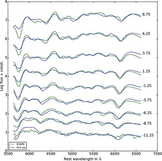
Synthetic spectra of the merger model (1.1 M⊙ + 0.9 M⊙) overplotted with the reconstructed spectra. The model spectra are in green and the reconstructions are in blue. The spectra are labelled with time relative to B-band maximum.
Pure deflagration models were suggested to be good candidates for (02cx-like) peculiar supernovae and, in fact, in Figs 3 and 4 we find them in the matching places of the PCA space. However, since again there are only a few objects of this group in our training set we do not expect to find very good fits. On the other hand, some pure deflagration models have 56Ni masses in the range of normal SNe Ia. Therefore, in principle, these qualify for the fainter normal ones as well. Fig. B3 shows model N150def, a typical example of relatively bright pure deflagration which disrupts the Chandrasekhar-mass white dwarf producing about 0.4 M⊙ of 56Ni. It is obvious that, in particular, past maximum the reconstructed spectra do not match the computed ones. For instance, the PCA reconstruction shows a Si ii feature at 6100 Å that is not present in the model spectra. At the same time, features in the model spectra at shorter wavelength, which are not present in the data, are weakened or even ignored in the reconstructions.
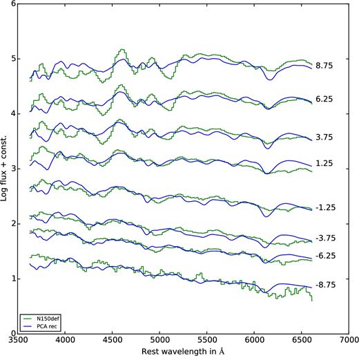
Same as Fig. B1, but for the pure deflagration model N150def.
Models in which the deflagration wave changes into a detonation during the explosion are also candidates for normal SNe Ia because they can, in principle, explain the range of observed luminosities. The model we show in Fig. B4 (N100) is a typical example of this class and was also used for a comparison with SN 2011fe by Roepke et al. (2012). The reconstruction works significantly better in this case, in particular for early epochs. This is not too surprising since at these epochs the model resembles major spectral features of normal SN Ia rather well (see also Fig. B9). Similarly, for model ‘N1600’ which, according to Figs 3 and 4, should be a good model for some of the observed explosions, also the reconstruction works properly, as shown in Fig. B5.
Finally, we compare two of the sub-Chandrasekhar-mass (pure detonation) models with their reconstruction. We have chosen the models with 0.97 M⊙ (Fig. B6) and 1.06 M⊙ (Fig. B7), respectively, since they produce Ni masses in the ballpark of normal SNe Ia. Not unexpectedly, the reconstruction is very good in both cases. There are small discrepancies for the spectra two to three weeks past maximum, but in general, both, spectral features and their evolution with time are reproduced.
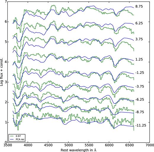
Same as Fig. B1, but for the sub-Chandrasekhar-mass model of 0.97 M⊙.
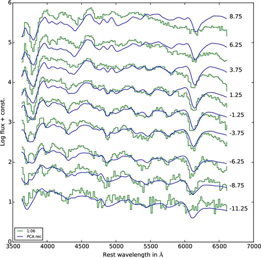
Same as Fig. B1, but for the sub-Chandrasekhar-mass model of 1.06 M⊙.
In conclusion, we have demonstrated that it is possible to represent the time sequences of model spectra by means of their principle components computed in the PCA space of the data. This works as long as the synthetic spectra bear some similarities with real supernova spectra but loses reliability if this is not the case or if the models are close to the edges of the PCA space populated by the data. The first problem becomes obvious when comparing synthetic spectra with their reconstructed counterparts at later times (t > 10 d past maximum) where our radiative-transfer modelling becomes less reliable.
Of course, a fair question is: how do model spectra compare with their nearest neighbours in PCA space? Ideally, one would hope that if in PCA space there are one or several real supernova nearby to a model their spectra should agree well. Since by means of PCA, we have constructed a metric space such a comparison can be done easily, and we show the results in Figs B8 through B10.
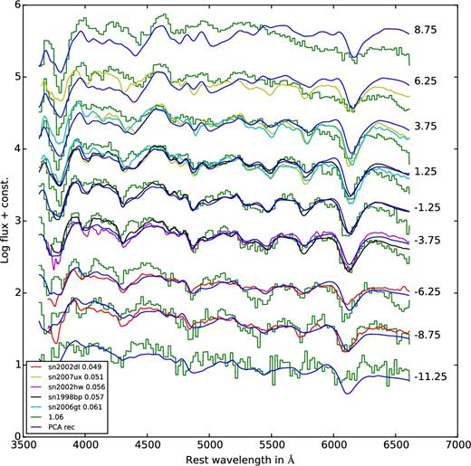
Synthetic spectra of the sub-Chandrasekhar-mass model of 1.06 M⊙ (in green) and their reconstruction (in blue) overplotted with spectra of nearby (in PCA space) observed supernovae. These supernovae a listed in the box in the lower left corner. The distance between the model and the SN in the PCA space is listed beside the name.
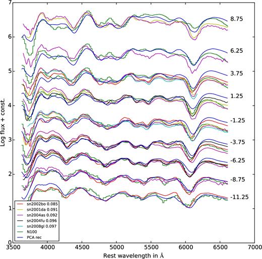
In Fig. B8, we play the game for the sub-Chandrasekhar-mass model of Fig. B6. We plot the five nearest (in PCA space) supernovae listed in the box in the left corner of the figure. The distances between the SNe and the model is listed in the legend beside their names. The model spectra are in green and their PCA reconstruction is in blue. The agreement is amazing, in particular for the pre-maximum spectra. Note that a close match to this model is also SN 2002dl, a 91bg-like supernova. Similarly, we find rather good agreement between the delayed-detonation model ‘N100’ (Fig. B4) and its reconstruction and some of its neighbours in PCA space (Fig. B9). This time, however, these neighbours are all normal or high-velocity SNe Ia in agreement with what we see in Figs 3 and 4. Note, however, that their distance to the model is quite large, indicating significant differences coming mainly from PC 4 and 5 which are not plotted. As our last example, we show the merger model of Fig. B1 in comparison with its nearest neighbours (Fig. B10). This time the fits are not quite as good, in particular at late times where also the reconstruction gets worse. This might be due to the approximations of the radiation transport procedure as all models differ from the corresponding reconstructions in a similar way.
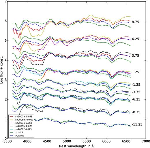
Same as B8, but for the violent-merger model (1.1 M⊙ + 0.9 M⊙).
All in all we find that our method passes also this final test rather well. It is not perfect and has to be applied with care, but it opens the possibility to compare models with observations in a more quantitative way and for large samples.


