


Abstract
The cosmological process of hydrogen (H i) reionization in the intergalactic medium is thought to be driven by UV photons emitted by star-forming galaxies and ionizing active galactic nuclei (AGN). The contribution of quasars (QSOs) to H i reionization at z > 4 has been traditionally believed to be quite modest. However, this view has been recently challenged by new estimates of a higher faint-end UV luminosity function (LF). To set firmer constraints on the emissivity of AGN at z < 6, we here make use of complete X-ray-selected samples including deep Chandra and new Cosmic Evolution Survey data, capable to efficiently measure the 1 Ryd comoving AGN emissivity up to z ∼ 5–6 and down to 5 mag fainter than probed by current optical surveys, without any luminosity extrapolation. We find good agreement between the logNH ≲ 21-22 cm−2 X-ray LF and the optically selected QSO LF at all redshifts for M1450 ≤ −23. The full range of the logNH ≲ 21-22 cm−2 LF (M1450 ≤ −17) was then used to quantify the contribution of AGN to the critical value of photon budget needed to keep the Universe ionized. We find that the contribution of ionizing AGN at z = 6 is as small as 1–7 per cent, and very unlikely to be greater than 30 per cent, thus excluding an AGN-dominated reionization scenario.
1 INTRODUCTION
The transition from the so-called dark ages to an ionized Universe involves the cosmological transformation of neutral hydrogen (H i), which mostly resides in the intergalactic medium (IGM), into an ionized state. Observations of distant active galactic nuclei (AGN) and gamma-ray bursts set the end of this process to z ∼ 6 (Fan et al. 2002; Kawai et al. 2006; McGreer, Mesinger & D'Odorico 2015), as confirmed by both theoretical calculations (Madau, Haardt & Rees 1999; Miralda-Escudé, Haehnelt & Rees 2000; Choudhury, Haehnelt & Regan 2009) and numerous observational astrophysical evidences (McGreer, Mesinger & Fan 2011; Pentericci et al. 2011; Planck Collaboration XVI 2014). All these studies broadly constrain the epoch of hydrogen reionization at 6 < z < 12, with a peak probability at |$z=8.8^{+1.7}_{-1.4}$| if instantaneous reionization is assumed (Planck Collaboration XIII 2016). The sources of ionizing photons (with energy greater than 13.6 eV, i.e. λ ≤ 912 Å) are traditionally believed to be star-forming galaxies (SFGs) and quasars (QSOs), though, which is the dominant one, is still a matter of considerable debate (Haiman & Loeb 1998; Schirber & Bullock 2003; Shankar & Mathur 2007; Robertson et al. 2010; Bouwens et al. 2012; Fontanot, Cristiani & Vanzella 2012). There is still room to gain a full comprehension of the overall picture of H i reionization. Indeed, one of the major open questions is how SFGs and QSOs completed the reionization at such early epochs since, given the observed properties of the two astrophysical populations, none of them can produce alone the total ionizing photon budget needed to end the reionization before redshift 6. This evidence supports contributions coming from alternative, more exotic, sources (Scott, Rees & Sciama 1991; Madau et al. 2004; Pierpaoli 2004; Volonteri & Gnedin 2009; Dopita et al. 2011).
The fraction of ionizing photons that freely escape each galaxy, fesc, is expected to be low, given that galaxies are characterized by observed soft spectra bluewards of Ly α due to the presence of cold gas and dust, which absorb most of the Lyman continuum emission (see e.g. Haehnelt et al. 2001). The fesc of SFGs is however still not highly constrained, even though the general idea is that it is much lower (i.e. fesc ∼ 0.1–0.2 at z ∼ 3–4, Shapley et al. 2006; Vanzella et al. 2010, and fesc ∼ 0.05–0.1 at z < 1, Bridge et al. 2010; Barger, Haffner & Bland-Hawthorn 2013) than the fesc of QSOs (for different results see e.g. Fontanot et al. 2014; Duncan & Conselice 2015; Rutkowski et al. 2016). Indeed, because of their observed UV hard spectra, some AGN are supposed to have large fesc, possibly reaching unity in the most luminous QSOs (see Guaita et al. 2016, for a significant direct detection at z = 3.46, and also the results of Cristiani et al. 2016).
Although QSOs have high 〈fesc〉, it is traditionally assumed that they are not the main contributors to H i reionization due to the steadily decreasing number density of AGN at z > 3 (e.g. Masters et al. 2012). Recently multiwavelength deep surveys at z > 3 (Glikman et al. 2011; Fiore et al. 2012; Giallongo et al. 2015) detected a larger number density of faint AGN at high redshifts, thus possibly implying a more substantial AGN contribution to H i reionization (Madau & Haardt 2015; Mao & Kim 2016, but see Georgakakis et al. 2015; Haardt & Salvaterra 2015; Weigel et al. 2015; Cappelluti et al. 2016).
However, strongly UV-emitting QSOs, showing optical blue spectra and broad emission lines (i.e. type-1 AGN), are only one class of the entire population of AGN, which also includes the type-2 AGN, characterized by red optical continuum and narrow emission lines. According to the standard AGN unified model (e.g. Urry & Padovani 1995), this kind of classification depends on the observer's line-of-sight with respect to an obscuring material, i.e. a dusty and probably clumpy torus. In a more realistic scenario, a contribution to the obscuration from the interstellar material of the hosting galaxy is also expected (e.g. Granato et al. 2004, 2006). Therefore, all AGN are alike but one source can appear as a type-1 or a type-2 depending on orientation and/or host-galaxy properties. Although in this scenario, type-2 AGN could appear as type-1 UV-emitting AGN under different line-of-sights, they should not be taken into account in the derivation of the UV background (UVB) as in any direction only type-1 AGN contribute to the UVB and, for isotropic arguments, their fraction should be the same (see also Cowie, Barger & Trouille 2009). In this framework, concerning the entire AGN population, fesc accounts for the fraction of unobscured AGN, since UV photons emitted by more obscured objects are likely to be absorbed locally within the host galaxy, and therefore do not contribute to the cosmic reionization (see also Georgakakis et al. 2015).
In the last decade, hard X-ray surveys have allowed the community to select almost complete AGN samples (including both type-1 and type-2 objects). Thanks to these studies, the evolution of the whole AGN population has been derived up to z ∼ 5 by many authors, all achieving fairly consistent results (Ueda et al. 2003, 2014; La Franca et al. 2005; Brusa et al. 2009; Civano et al. 2011; Kalfountzou et al. 2014; Vito et al. 2014; Aird et al. 2015a,b; Georgakakis et al. 2015; Miyaji et al. 2015). The X-ray spectra of AGN show a wide range of absorbing column densities (20 < log NH < 26 cm−2), with optically classified type-1 AGN (i.e. QSOs) believed to broadly correspond to those AGN with the lowest NH distributions, typically |$\log N\rm _H<$| 21 cm−2, though the exact correlation between X-ray and optical classifications is still quite debated (Lusso et al. 2013; Merloni et al. 2014). In this framework, the X-ray luminosity function (XLF) of the AGN with low column densities (log NH < 21–22 cm−2) could be potentially used as an unbiased proxy of the ionizing AGN population (i.e. QSOs), where 〈fesc〉 ∼ 1 is expected. On the contrary, at larger column densities, fesc should sharply decrease down to zero. The advantage of X-ray selection is that it is less biased towards line-of-sight obscuration, extinction and galaxy dilution, especially at high z (where harder portion of the spectra are probed), assuring a better handle on the faint-end of the AGN luminosity function (LF) compared to UV/optically selected samples. Additionally, at low luminosities, the standard optical colour–colour QSO identification procedure becomes less reliable, because QSO emission is superseded by the hosting galaxy. Moreover, moving to high redshifts, stars can be misinterpreted as QSOs: consequently, low-luminosity optical surveys have so far produced disagreeing QSO LFs (QLFs; see Glikman et al. 2011; Ikeda et al. 2011; Masters et al. 2012).
In this work, we make use of the latest results on the X-ray AGN number densities including deep Chandra and Cosmic Evolution Survey – COSMOS – data (e.g. Ueda et al. 2014; Vito et al. 2014; Marchesi et al. 2016b). Our aim is to provide more stringent constraints on the AGN contribution to the H i reionization. To achieve this, we investigate whether the low NH XLF can be used as an unbiased proxy to derive robust estimates of the QSO ionizing emissivity (for a similar approach at 3 < z < 5, see Georgakakis et al. 2015). We will study the AGN LF up to redshift ∼6 over a broad range of 2–10 keV band luminosities, 1042 < LX < 1046.5 erg s−1, 5 mag fainter than the UV/optically selected LFs, thus providing more stringent constraints on the density of low-luminosity QSOs.
The paper is organized as follows: in Section 2, we describe the UV/optical and X-ray AGN LFs used in our study. In Section 3, we compare the UV/optical and the X-ray LFs in order to determine which sub-sample of the XLF better describes the UV/optical QLF. Section 3 also focuses on the faint end of the UV LF at z > 4. Section 4 describes the computation of the ionizing AGN emissivity. The discussion is presented in Section 5 and the conclusions in Section 6. Unless otherwise stated, all quoted errors are at the 68 per cent (1σ) confidence level. Throughout the paper we assume a standard cosmology, with parameters H0 = 70 km s−1Mpc−1, Ωm = 0.3 and |$\Omega _\Lambda = 0.7$|.
2 DATA
We start off by comparing a relevant number of complete UV/optically selected QSO and X-ray-selected AGN samples and LFs.
2.1 QSO UV luminosity functions
All the optical/UV QLFs were converted into AB absolute magnitude at 1450 Å, M1450, using the expressions Mi(z = 2) = Mg(z = 2) − 0.25 and Mi(z = 2) = M1450(z = 0) − 1.486 (see Ross et al. 2013, equations 8 and 9), and are shown in Fig. 1 in seven representative redshift bins.
SDSSQS: in the redshift range 0.3 < z < 5.0, we use the absolute i-band (7470 Å) binned QLF from the Sloan Digital Sky Survey Data Release 3 (SDSS DR3, Richards et al. 2006). The sample consists of 15 343 QSOs and extends from i = 15 to 19.1 at z ≲ 3, and to i = 20.2 at z ≳ 3.
SDSS-2SLAQ: the 2dF-SDSS LRG And QSO survey (2SLAQ; Croom et al. 2009) at 0.4 < z < 2.6 has 12 702 QSOs with an absolute continuum limiting magnitude of Mg(z = 2) < −21.5.
SDSS-III/BOSS QSO survey (DR3): for 0.68 < z < 4 down to the limiting extinction-corrected magnitude g = 22.5, Palanque-Delabrouille et al. (2013) used variability-based selection to measure the QLF.1The targets were shared between SDSS-III: Baryon Oscillation Spectroscopic Survey (BOSS21) and the Multiple Mirror Telescope (MMT), yielding a total of 1877 QSOs.
SDSS-III/BOSS QSO survey (DR9): the optical QLF in the range 2.2 < z < 3.5 has been studied also by Ross et al. (2013), who targeted g < 22 QSOs in the BOSS DR9 footprint, achieving a total of 23 301 QSOs sampled in the absolute magnitude −30 ≤ Mi ≤ −24.5.
COSMOS-Masters+12: the rest-frame UV QLF in the COSMOS at 3.1 < z < 3.5 and 3.5 < z < 5 was investigated by Masters et al. (2012), which reached the limiting apparent magnitude of IAB = 25. This sample of 155 likely type-1 AGN is highly complete above z = 3.1 in the HST-Advanced Camera for Surveys (ACS) region of COSMOS.
COSMOS-Ikeda+11: the same area of the COSMOS field was studied by Ikeda et al. (2011) also, in order to probe the faint-end of the QLF at 3.7 ≲ z ≲ 4.7. They reached 5σ limiting AB magnitudes u* = 26.5, g΄ = 26.5, r΄ = 26.6 and i΄ = 26.1. They selected 31 QSO candidates using colours (r΄ − i΄ versus g΄ − r΄) and found eight spectroscopically confirmed QSOs at z ∼ 4.
COSMOS-Ikeda+12: Ikeda et al. (2012) searched in a similar way candidates of low-luminosity QSO at z ∼ 5 using the colours i΄ − z΄ versus r΄ − i΄. Their spectroscopic campaign confirmed one type-2 AGN at z ∼ 5.07 and set upper limits on the QLF.
DLS-NDWFS: Glikman et al. (2010) developed a colour selection (R − I versus B − R) using simulated QSO spectra. This technique was then used by Glikman et al. (2011) to build the z ∼ 4 UV LF using parts of the Deep Lens Survey (DLS) and National Optical Astronomy Observatory (NOAO) Deep Wide-Field Survey (NDWFS), finding 24 QSOs with 3.74 < z < 5.06, down to M1450 = −21 mag.
SDSS STRIPE82-McGreer+13: at 4.7 < z < 5.1, we use the QLF investigated by McGreer et al. (2013), whose sample has a total of 52 AGN at a limiting magnitude of iAB = 22.
SDSS STRIPE82-Jiang+09: Jiang et al. (2009) discovered six QSOs at z ∼ 6, four of which comprise a complete flux-limited sample at 21 < zAB < 21.8.
Subaru high-z QSO survey: the Subaru high-z QSO survey provided an estimate of the faint end of the QLF at z ∼ 6. Kashikawa et al. (2015) have a sample of 17 QSO candidates at limiting magnitude zR < 24.0, but for 10 of them do not have spectroscopic follow-up; therefore, their faintest bin might be a lower limit on the QLF.
Cosmic Assembly Near-infrared Deep Extragalactic Legacy Survey (CANDELS) Great Observatories Origin Deep Survey - South (GOODS-S)-S: the CANDELS GOODS-S field has yielded 22 AGN candidates at 4 < z < 6.5, five of which have spectroscopic redshifts, down to a mean depth of H = 27.5 (Giallongo et al. 2015). The resulting UV LF lies in the absolute magnitude interval − 22.5 ≲ M1450 ≲ −18.5.
IMS-SA22: recently, Kim et al. (2015) searched for high-z QSOs in one field (i.e. SA22) of the Infrared Medium-deep Survey (IMS). The reached J-band depth corresponds at z = 6 to M1450 ≃ −23 mag. They found a new spectroscopically confirmed QSO at z = 5.944, and other six candidates using colour selection.
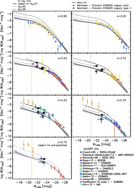
AGN LFs at different redshifts as a function of the absolute AB magnitude M1450. Symbols and colours used for the optical/UV samples are reported in the legend (for more details, see Section 2.1). At z > 3, we show the new measure of the 2–10 keV LF of type-1 (black open squares) and the whole AGN sample (black filled squares) made by the Chandra COSMOS Legacy Survey (Marchesi et al. 2016b), and converted into UV magnitudes (see Section 3). The plot also shows other recent estimates of the 2–10 keV LFs (converted into UV magnitudes) of unobscured AGN, i.e. log NH < 21 cm−2 (Ueda et al. 2014, black solid line) and log NH < 22 cm−2 (Ueda et al. 2014, black dotted line), and inclusive of Compton-thick AGN (Ueda et al. 2014; Vito et al. 2014, black dashed and triple-dot–dashed lines, respectively). The grey shaded area indicates the effect of changing the LX–L2500 (see text for details) relation on the X-ray log NH < 21 cm−2 LF. The X-ray luminosity functions are drawn in grey when they have been extrapolated above existing data. The green dashed vertical line represents the evolution of the break magnitude M* at 1500 Å of the galaxy UV LF (Parsa et al. 2016).
2.2 X-ray luminosity functions
We have based our analysis on the Ueda et al. (2014) XLF, which is obtained using 4039 sources from 13 different X-ray surveys performed with Swift/Burst Alert Telescope (BAT), MAXI, ASCA, XMM–Newton, Chandra and ROSAT. These sources have been detected in the soft (0.5–2 keV) and/or hard (>2 keV) X-ray bands. The 2–10 keV LF has been computed in the redshift range 0 < z < 5 and in the luminosity range 42 |$<\log L\rm _X<$| 46.5 erg s−1. The faint end of this range is luminous enough (i.e. an order of magnitude larger) to exclude the contribution to the X-ray emission of both X-ray binaries and hot extended gas (see e.g. Lehmer et al. 2012; Basu-Zych et al. 2013; Kim & Fabbiano 2013; Civano et al. 2014). Indeed, the threshold of ∼1041 erg s−1 translates, according to Lehmer et al. (2012, see their equation 12), into a star-formation rate (SFR) of ∼ 10–100 M⊙ yr−1.
Ueda et al. (2014) found that the shape of the XLF significantly changes with redshift: in the local Universe, the faint-end slope (i.e. below the XLF break) is steeper than in the redshift range 1 < z < 3. Ueda et al. (2014) computed the XLF in various absorption ranges (i.e. at different NH): they confirmed the existence of a strong anticorrelation between the fraction of absorbed objects and the 2–10 keV luminosity. At high luminosities, the majority of AGN are unabsorbed, while moving to low luminosities (|$\log L\rm _X<$| 43.5 erg s−1 in the redshift range 0.1 < z < 1) the contribution of absorbed AGN to the XLF becomes dominant. Moreover, this trend evolves with redshift, maintaining the same slope but shifting towards higher luminosities (see also La Franca et al. 2005; Hasinger 2008).
Vito et al. (2014) computed the 2–10 keV AGN LF in the redshift range 3 < z ≤ 5 from a sample of 141 sources selected in the 0.5–2 keV band. The sample was obtained combining four different surveys down to a flux limit ∼ 9.1 × 10⁻¹⁸ erg s−1 cm−2. In this redshift range, the XLF is well described by a pure density evolution model, i.e. there is no luminosity dependence on the shape of the LF at different redshifts. In this work, the whole XLF by Vito et al. (2014) has been used without separating according to the NH classification.
The Chandra COSMOS Legacy (Civano et al. 2016; Marchesi et al. 2016a) z ≥ 3 sample (Marchesi et al. 2016b) contains 174 sources with z ≥ 3, 27 with z ≥ 4, nine with z ≥ 5 and four with z ≥ 6. Eighty-seven of these sources have a reliable spectroscopic redshift, while for the other 87 a photometric redshift has been computed (Salvato et al. 2011). The photo-z mean error is ∼5–10 per cent, with 60 per cent of the sample having uncertainties less than 2 per cent, while for 10 per cent of the sample the uncertainties are greater than 20 per cent. The 2–10 keV Chandra COSMOS Legacy z ≥ 3 sample is complete at |$L\rm _{X}>10^{44.1}$| erg s−1 in the redshift range 3 < z < 6.8; at lower luminosities (1043.55 < LX < 1044.1 erg s−1), the sample is complete in the redshift range 3 < z < 3.5. For the purposes of this work, we computed the space densities also at z = 3.75, in the luminosity range 1043.7 < LX < 1044.1 erg s−1, and at z = 4.25, in the luminosity range 1043.8 < LX < 1044.1 erg s−1. The Chandra COSMOS Legacy z ≥ 3 sample has also been divided into two sub-samples: one is made by 85 type-1 AGN, on the basis of their spectroscopical classification, or, when only photo-z was available, with a spectral energy distribution (SED) fitted with an unobscured AGN template; the second sub-sample is formed by the 89 optically classified type-2 AGN, either without evidence of broad lines in their spectra, or SED best-fitted by an obscured AGN or a galaxy template (for the description of the optical sources classification, see Marchesi et al. 2016a).
3 Comparison between UV/optical and X-ray LFs
3.1 Converting the X-ray into UV
3.2 Comparing the converted XLFs
In Fig. 1 we show the AGN UV LF, as measured by the optically selected QLFs, already described in Section 2.1, together with the XLF by Marchesi et al. (2016b, black open squares for type-1 AGN and black filled squares for the whole sample). We also show the Vito et al. (2014) XLF (black triple-dot–dashed line) and the Ueda et al. (2014) XLF in three different NH regimes: log NH < 21 cm−2 (black solid line); log NH < 22 cm−2 (black dotted line); log NH < 26 cm−2 (whole AGN population, i.e. including Compton-thick sources, black dashed line). All the XLFs have been plotted only in the redshift and X-ray luminosity ranges where data exist. At z = 5.75, the Ueda et al. (2014) XLF has been extrapolated (it has been originally computed in the redshift range 0 < z < 5; see Section 2.2), and then it has been drawn in grey in Fig. 1. The grey shaded region shows the effect of changing the relations between L2 keV and L2500 in the conversion of the Ueda et al. (2014) log NH < 21 cm−2 XLF: besides the relation by Lusso et al. (2010), the relation found by Steffen et al. (2006, see their equation 1b) was used to obtain the upper and lower limits on this area.
It is worth noticing the perfect agreement between Vito et al. (2014) and Ueda et al. (2014) XLF having log NH < 26 cm−2 over the whole luminosity range in which both XLFs exist and in all the redshift bins with z > 3, taken into account in our analysis. As noted in Section 2.2, in this work we used the XLF computed by Vito et al. (2014) without separating according to the NH classification, hence this XLF describes the whole X-ray-emitting AGN population. Also the new measures from the Chandra COSMOS Legacy Survey z > 3 sample are in good agreement with the above two XLFs at all redshifts, given the current uncertainties both in X-ray luminosity and density. The most important contribution coming from the Chandra COSMOS Legacy Survey z > 3 sample is that it confirms the extrapolation of the Ueda et al. (2014) XLF at luminosities LX ∼ L* and z > 5 (see Fig. 1), therefore supporting the use of the Ueda et al. (2014) XLF also for z ∼ 5–6, which is one of the key epochs for reionization studies. Given the good agreement between these different X-ray LFs, independently computed, we claim that the AGN description coming from the X-ray-selected samples is coherent and robust, clearly confirming the global ‘downsizing’ evolution, where more luminous AGN have their number density peak at higher redshifts compared with less luminous ones.
There are, however, some recent estimates of the XLF (Buchner et al. 2015; Fotopoulou et al. 2016) which predict a higher (∼1 dex) number of low-luminosity X-ray-selected AGN, particularly at high redshift. This evidence is in contrast with the findings of a steep declining of the AGN number density moving to higher redshifts (Ueda et al. 2014; Vito et al. 2014; Aird et al. 2015a,b; Georgakakis et al. 2015; Miyaji et al. 2015). We will discuss later in Section 3.3 how the predicted number density of UV-selected AGN at high redshift changes assuming different X-ray parent populations.
3.3 Comparing the converted XLFs and the UV LF
As shown in Fig. 1, there is a fairly good agreement between the UV/optical binned QLFs and the 2–10 keV log NH < 21 and log NH < 22 cm−2 AGN LFs up to z ∼ 6, in the luminosity range of the break and beyond (i.e. M1450 ≤ −23). As expected, this result is in agreement with the unification model where (as discussed in the Introduction) the X-ray log NH ≲ 21–22 cm−2 AGN population should correspond to the UV/optically selected QSOs (see also Cowie et al. 2009). We note that this matching between optical QSOs and X-ray log NH ≲ 21-22 cm−2 population up to z = 6 is also in agreement with what was found by Risaliti & Lusso (2015), who showed that αOX(LX) is redshift-independent, and can therefore be used to derive a cosmological distance indicator. Indeed, this matching implies, as we have assumed, that a change of the relation between L2500 and L2 keV with redshift is not required.
The determination of the AGN LF faint end is one of the still open problems in extragalactic astronomy, and it translates into a poor knowledge of the AGN demography and evolution, especially when moving at z > 4.
At luminosities lower than the break (i.e. M1450 ≥ −23), a good agreement between the UV/optical and X-ray samples is found only up to redshift ∼4, while at higher redshifts, the log NH ≲ 22 cm−2 XLF of Ueda et al. (2014) underpredicts up to a factor of ∼1 dex the LFs by Glikman et al. (2011) and Giallongo et al. (2015), which were both measured using rest-frame UV-selected samples. This disagreement between X-ray and rest-frame UV-selected AGN samples has been recently found also by Vito et al. (2016), who derived an upper limit on the AGN XLF by stacking the X-ray counts in the Chandra Deep Field - South (CDF-S) 7 Ms, which is the deepest X-ray survey to date. In what follows, we discuss a few possible scenarios that may explain the origin of these discrepancies.
As already discussed by Giallongo et al. (2015), it could be possible that in the UV fluxes of their sample the contribution of the stellar emission of the hosting galaxy is not negligible. Indeed, as shown in Fig. 2 (left-hand panel, red solid line) the log NH < 23 cm−2 XLF2 (corresponding to the typical NH value measured in the sample of Giallongo et al. 2015) could reproduce the Glikman et al. (2011) and Giallongo et al. (2015) measures, once typical L* galaxy luminosities (−21.5 < M1450 < −19.5 at z = 4.25, orange dashed horizontal lines in Fig. 2) are added to the AGN luminosity. The left-hand panel of Fig. 2 also shows for guidance the break magnitude at 1500 Å of the galaxy UV LF (green dashed vertical line; Parsa et al. 2016). A non-negligible galaxy contribution can be also related to a scenario in which the faint (not heavily absorbed) AGN population with log NH ≲ 23 cm−2 could, through outflows and mechanical feedback, increase the fesc of SFGs by cleaning the environment and enhancing the porosity of the Interstellar medium (ISM, see e.g. Giallongo et al. 2015; Smith et al. 2016). This mechanism could be rather effective at higher redshift as the UV emission could be produced more efficiently by Pop III stars (Kimm et al. 2016).
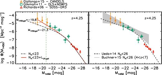
UV LF at redshift 4.25. Left: the faint end of the UV LF measured by UV/optically selected samples of Giallongo et al. (2015, orange triangles) and Glikman et al. (2011, green squares) could be described by the log NH < 23 cm−2 XLF of Ueda et al. (2014) adding a UV contribution arising from the luminosity of the host galaxy with magnitudes in the range −21.5 < M1450 < −19.5, which are typical of the galaxy LF break luminosity at this redshift (M1500 ∼ −20.8, green dashed vertical line; Parsa et al. 2016). A Gaussian convolution that accounts for the observed spread (σ ∼ 0.4) in the relation LX–L2500 (red line) has also been included. Right: comparison of the UV/optically selected samples and two different XLFs that consider also the contribution of the Compton-thick AGN (log NH < 26 cm−2), namely the Ueda et al. (2014, black dashed line) and Buchner et al. (2015, grey shaded area).
An alternative scenario is that at high redshift the UV-selected samples are not only associated with X-ray log NH ≲ 22 cm−2 AGN, but also with heavily X-ray-absorbed AGN (log NH > 25 cm−2). If the AGN population which mostly contribute to the ionizing background have greater NH values than that considered in our minimal baseline model (which have been chosen to match the optical/UV LFs at z < 4), then the fesc does not become zero rapidly for NH > 1022 cm−2. Therefore, the AGN contribution to UV emission would be enhanced. Indeed, in this case the underprediction by the log NH < 26 cm−2 XLF of the UV LFs reduces to ≲ 0.5 dex. This scenario is rather unlikely. Indeed, although there is evidence that the ratio between hydrogen column density and extinction in the V band (i.e. the NH/AV ratio) could be larger than Galactic in AGN (see e.g. Maiolino et al. 2001; Burtscher et al. 2016), it has been shown that all AGN with NH > 1022 cm−2 have AV > 5 (Burtscher et al. 2016); therefore, the UV photons will be likely absorbed within the host galaxy and do not contribute to the cosmic ionization. Moreover, Burtscher et al. (2016) showed that if accurate X-ray and optical analysis is carried out, an agreement between the X-ray and optical classification is found.
As introduced in Section 3.2, recently it has been claimed that the XLF (Buchner et al. 2015; Fotopoulou et al. 2016) has a higher density of low-luminosity AGN compared to the estimates from Ueda et al. (2014), Miyaji et al. (2015), Aird et al. (2015a), Aird et al. (2015b), Georgakakis et al. (2015) and Vito et al. (2014). The right-hand panel of Fig. 2 shows the whole AGN XLF (i.e. including the Compton-thick population) by Buchner et al. (2015), converted into UV magnitudes (grey shaded area), together with the corresponding XLF by Ueda et al. (2014, dashed black curve) and the UV/optically selected samples at z = 4.25. The two XLFs were converted into UV according to our standard procedure highlighted in Section 3.1. Concerning the X-ray population with log NH < 26 cm−2, the XLF by Buchner et al. (2015) is indeed ∼1 dex higher than the XLF by Ueda et al. (2014) and this factor is enough to reproduce the UV/optically selected samples. None the less, it must be considered that this agreement is found only if the heavily X-ray-absorbed AGN population is also included. The uncertainties are quite large (∼1 dex in density and the redshift bin is very broad, 4 < z < 7), and Buchner et al. (2015) state that this is the reason for possibly not finding a steep decline with redshift in their AGN space density.
In summary, we found that there is a discrepancy at the faint-end of the UV LF between the measures derived using direct UV data and the prediction of the X-ray log NH ≲ 22 cm−2 AGN LF at z > 4. This discrepancy, which is absent at lower redshifts, can be attributed either to a small contribution of UV emission in the AGN host galaxy of the order of the galaxy UV L* or, unlikely, to a substantial contribution to the UVB coming from an X-ray-absorbed population whose density and escape fraction, consequently, should have been underestimated by most of the previous studies.
However, inside the AGN unified models, it should be remembered (see Introduction) that, for isotropic reasons, we are interested in the unabsorbed log NH < 22 cm−2 population as measured along the line-of-sight, since the fraction of ionizing AGN should be the same for any observer in the Universe.
4 QSO UV EMISSIVITY
As discussed at the beginning of Section 3.3, the good agreement between the optical QLF and the log NH ≲ 21–22 cm−2 XLF indicates that this XLF is a good proxy to estimate the space density of ionizing AGN (i.e. the QSOs). Therefore, we will assume that the log NH ≲ 21–22 cm−2 AGN have 〈fesc〉 = 1, while the rest of the population has rapidly decreasing fesc as NH increases.
Most of the previous studies on the estimate of the ionizing background produced by QSOs have used UV/optically selected sample and, as shown in Fig. 1, they needed to extrapolate the QLF below the break luminosity (see e.g. Khaire & Srianand 2015; Madau & Haardt 2015). On the contrary, the use of the log NH < 21 cm−2 XLF allows us to measure the QSO emissivity without any extrapolation at low luminosities down to 5 mag fainter than optical surveys and up to z ∼ 5.
4.1 Comparing optical and X-ray emissivities
Fig. 3 (left-hand panel) shows the evolution of the comoving ionizing emissivity ε912 as a function of redshift for the log NH < 21 and log NH < 22 cm−2 X-ray population (solid and dotted black lines, respectively). When the XLF has been extrapolated, i.e. at z > 5, the emissivities are drawn in grey. The above-computed X-ray emissivities are reported in Table 1 up to z = 7.
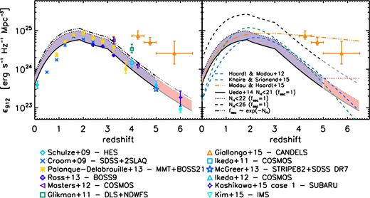
Redshift evolution of the hydrogen ionizing emissivities, ε912(z). Left: ε912 computed using the UV/optical binned QLF described in Section 2.1, colours and symbols are reported in the legend. The solid and dotted black lines are the ε912 computed (with fesc = 1) from the 2–10 keV LF by Ueda et al. (2014, solid line for the log NH < 21 cm−2, black dotted for log NH < 22 cm−2). The triple-dot–dashed black line shows the resulting emissivity computed assuming |$f_{\rm {esc}}\sim {\rm e}^{-N_{\rm H}}$| (see text for more details). The emissivities are drawn in grey when XLFs are extrapolated. The shaded area shows our best estimate of the UV ionizing AGN emissivity, which should lie in between the two limits of log NH < 21 and log NH < 22 cm−2. When the XLFs are extrapolated, the shaded area is plotted in pink. Right: the black dashed line is ε912 computed from the 2–10 keV LF by Ueda et al. (2014) inclusive of Compton-thick sources assuming an extreme fesc = 1 (see text for more details). The red dotted horizontal line shows the upper limit on the log NH < 22 cm−2 population assuming that the XLF remains constant for z > 5. The other curves are the prediction of the evolution of the emissivity with redshift from Haardt & Madau (2012, blue dashed), Khaire & Srianand (2015, green dashed) and Madau & Haardt (2015, orange triple-dot–dashed).
Redshift evolution of emissivities at 912 Å obtained integrating the XLFs of Ueda et al. (2014) with equation (4) with log Lmin = 27.22 erg s−1 Hz−1. Columns are (1) redshifts, (2) logarithm of the H i ionizing emissivities computed from the X-ray log NH < 21 cm−2 AGN, (3) from the log NH < 22 cm−2 AGN and (4) the whole X-ray AGN population. The emissivities in columns (2) and (3) have been computed assuming fesc = 1, whereas the ε912 in column (4) has been weighted with fesc exponentially dependent on NH. Columns (2)–(4) are in units erg s−1 Hz−1 Mpc−3.
| z | log ε912 | ||
|---|---|---|---|
| (NH < 1021) | (NH < 1022) | (NH < 1026) | |
| fesc = 1 | fesc = 1 | fesc ∼ exp (−NH) | |
| (1) | (2) | (3) | (4) |
| 0.0 | 23.62 | 23.84 | 23.89 |
| 0.2 | 23.91 | 24.14 | 24.20 |
| 0.4 | 24.15 | 24.39 | 24.44 |
| 0.6 | 24.33 | 24.57 | 24.63 |
| 0.8 | 24.47 | 24.71 | 24.77 |
| 1.0 | 24.58 | 24.82 | 24.88 |
| 1.2 | 24.65 | 24.90 | 24.95 |
| 1.4 | 24.70 | 24.94 | 25.00 |
| 1.6 | 24.74 | 24.97 | 25.03 |
| 1.8 | 24.76 | 24.99 | 25.05 |
| 2.0 | 24.72 | 24.96 | 25.02 |
| 2.2 | 24.67 | 24.92 | 24.98 |
| 2.4 | 24.64 | 24.88 | 24.94 |
| 2.6 | 24.60 | 24.84 | 24.90 |
| 2.8 | 24.56 | 24.81 | 24.86 |
| 3.0 | 24.53 | 24.77 | 24.83 |
| 3.2 | 24.42 | 24.67 | 24.72 |
| 3.4 | 24.31 | 24.56 | 24.62 |
| 3.6 | 24.20 | 24.45 | 24.51 |
| 3.8 | 24.09 | 24.34 | 24.40 |
| 4.0 | 23.99 | 24.24 | 24.30 |
| 4.2 | 23.89 | 24.14 | 24.20 |
| 4.4 | 23.79 | 24.04 | 24.10 |
| 4.6 | 23.70 | 23.94 | 24.00 |
| 4.8 | 23.60 | 23.85 | 23.91 |
| 5.0 | 23.51 | 23.76 | 23.82 |
| 5.2 | 23.42 | 23.67 | 23.73 |
| 5.4 | 23.34 | 23.59 | 23.65 |
| 5.6 | 23.25 | 23.51 | 23.57 |
| 5.8 | 23.17 | 23.42 | 23.49 |
| 6.0 | 23.09 | 23.38 | 23.41 |
| 6.2 | 23.02 | 23.27 | 23.33 |
| 6.4 | 22.95 | 23.20 | 23.26 |
| 6.6 | 22.87 | 23.12 | 23.18 |
| 6.8 | 22.80 | 23.05 | 23.11 |
| 7.0 | 22.73 | 22.98 | 23.04 |
As a comparison, we also report in the left-hand panel of the same figure other measures which we have derived using the UV/optically selected QSO samples (see Section 2.1). We set Lmin as the faintest luminosity bin available in each survey. In particular, when integrating the XLF, we set log Lmin = 27.22 erg s−1 Hz−1 (i.e. log LX = 42 erg s−1). The choice of not extrapolating the LF in a luminosity range not yet sampled by current surveys is conservative and implies that the derived QSO ionizing emissivities are, strictly speaking, lower limits. Indeed, the adoption of the XLF as an unbiased representation of the UV/optical QLF allows us to extend the lower luminosity limits of the optical LFs (see Fig. 1) and then reach fainter Lmin in the integration of equation (4). When the XLF has been extrapolated, i.e. at z > 5, we have assumed the evolution implied by Ueda et al. (2014) and we have solved equation (4) setting Lmin as previously done.
Given the definition in equation (4), the emissivity is proportional to the area beneath the curve L × Φ(L). Due to the double-power-law shape of the LF, L × Φ(L) presents a maximum located in the luminosity break region L*. Therefore, at each redshift the leading contribution to emissivity comes from AGN at L*, and this is true as far as the faint-end slope of the LF is not too steep.
In order to show the emissivity at z = 0 derived from the optically selected QLF, we used the B-band double-power-law QLF from Schulze, Wisotzki & Husemann (2009, cyan diamond with error bars; for the LF see their table 4).3 At z > 4, we also show the results from Giallongo et al. (2015, orange triangles with error bars).
The contribution of the X-ray log NH < 21 cm−2 population should be considered as a lower limit to the AGN ionizing emissivity (black solid line in Fig. 3); in fact, the 21 < log NH < 22 cm−2 AGN could also contribute significantly. Inside our minimal model, an upper limit to the QSO emissivity can be derived (black dotted line in Fig. 3) under the hypothesis of 〈fesc〉 = 1 up to log NH = 22 cm−2 and then sharply zero for the rest of the AGN. We tested how strong is this last approximation on the upper limit to the AGN contribution to the emissivity by assigning an fesc depending on the column density NH. Indeed, a relation between the escape fraction and the extinction of the type |$f_{\rm {esc}} \propto {\rm e}^{-A_V}$| is expected (Mao et al. 2007). Therefore, in a less simplified (and more realistic) model, assuming a constant NH/AV ratio, the escape fraction is expected to exponentially depend on the NH. In this scenario, an escape fraction equal to unity at log NH = 21 cm−2 will drop to ∼0.37 at log NH = 22.5 cm−2 and to ∼5 × 10⁻⁵ already at log NH = 23.5 cm−2. This calculation is reported in Table 1 and is shown in Fig. 3 (left-hand panel) as a triple-dot–dashed black line. The emissivity computed assuming the exponential dependence on NH is only slightly enhanced (∼15 per cent) with respect to the first simplified approximation of fesc sharply zero for NH > 1022 cm−2. An almost identical result is obtained also assuming fesc = 1 up to log NH = 22 cm−2 and an additional constant fesc = 0.1 for the 22 < log NH < 26 cm−2 AGN population. Since the scenario in which the fesc is dependent on NH does not alter significantly our initial simplified and rather strong approximation that the fesc sharply drop to zero for all AGN having log NH > 22 cm−2, we will continue to use as upper limit on the AGN emissivity the one calculated assuming fesc = 1 up to log NH = 22 cm−2 only.
As expected, the estimates obtained using the X-ray log NH < 21 and log NH < 22 cm−2 LFs are in good agreement with most of the estimates coming from the optical/UV QLFs, where available. At variance, as already noticed in Section 3, the measures at z > 4 by Glikman et al. (2011) and Giallongo et al. (2015) are up to a factor of ∼8 larger than the other estimates, obtained both from optical and X-ray data. This difference was also pointed out by Georgakakis et al. (2015) who integrated the XLF in the range 3 < z < 5 (see Section 3 for a discussion on possible sources of this discrepancy). The violet shaded area, which is our best estimate of the AGN ionizing emissivity, is the region included between the predictions of the log NH < 21 and log NH < 22 cm−2 populations. The shaded area is plotted in pink when the XLFs have been extrapolated (z > 5).
Fig. 3 (right-hand panel) shows the contribution to the emissivity produced by AGN at different NH: the log NH < 21 and log NH < 22 cm−2 populations (same legend as the left-hand panel) and the whole AGN population, including also Compton-thick sources (Ueda et al. 2014, black dashed line), under the very extreme and unphysical assumption that all AGN (up to NH = 1026cm−2) have fesc = 1. Again, the emissivity has been drawn in grey when extrapolated at z > 5. The dotted red horizontal line plotted in the right-hand panel of Fig. 3 shows, according to our analysis, the UV ionizing AGN emissivity upper limit in the redshift range 5 < z < 6, obtained under the two assumptions that AGN with log NH < 22 cm−2 contribute significantly to reionization (〈fesc〉 = 1) and that the XLF remains constant for z > 5. In this case, the discrepancy between our upper limits and the results of Giallongo et al. (2015) is a factor of ∼4. Even considering the contribution of the very absorbed AGN, a discrepancy of a factor ∼3 with the results of Giallongo et al. (2015) still remains.
For reference, we also plot the evolution of the comoving emissivity as a function of redshift from Haardt & Madau (2012, blue dashed line; their equation 37; see also Hopkins, Richards & Hernquist 2007), Khaire & Srianand (2015, green dashed line; equation 6 of their work) and Madau & Haardt (2015, orange triple-dot–dashed line; equation 1 of their work). We note that the agreement between our best estimate and other emissivities in literature, which have been derived under different assumptions, is quite good. As shown in Fig. 3, we found a high integrated local AGN emissivity as recently proposed by Madau & Haardt (2015), a fact that can reduce the photon underproduction crisis 4 (Kollmeier et al. 2014, see also Shull et al. 2015 and Gaikwad et al. 2016). A precise analysis of this issue is however beyond the scope of this work.
Our best estimate is in agreement at z < 2 with the ε912 proposed by Madau & Haardt (2015), while the emissivities proposed by Haardt & Madau (2012) and Khaire & Srianand (2015) are in fair agreement at 2 < z < 6 with our best estimate given the current uncertainties. In particular, the ε912 of the log NH < 22 cm−2 agrees with the Khaire & Srianand (2015) estimate at 2 < z < 4.5 while it is higher at z > 5. The emissivity that we obtain considering only the log NH < 21 cm−2 population, which represents our lower limit, is the lowest estimate at 2 < z < 5 and agrees with the emissivity of Haardt & Madau (2012) at z > 6. At variance, the QSO emissivity given by Madau & Haardt (2015) is definitely larger than our estimate at z > 3, as their analysis is based on the results by Giallongo et al. (2015).
5 DISCUSSION
As discussed in the previous section, with our calculations we propose that the range of possible values of the QSO ionizing emissivity should lie in the shaded area highlighted in Fig. 3, i.e. in between the two limits obtained considering the AGN population with log NH < 21 and log NH < 22 cm−2(solid and dotted black lines).
We now compute the possible contribution of X-ray log NH < 21 and log NH < 22 cm−2 AGN to the reionization of H i residing in the IGM. The transition from a neutral to a fully ionized IGM is statistically described by a differential equation for the time evolution of the volume-filling factor of the medium, Q(z) (see e.g. Madau et al. 1999). Q(z) quantifies the level of the IGM porosity created by H i ionization regions around radiative sources such as QSOs and SFGs. The evolution of Q(z) is given by the injection rate density of ionizing radiation minus the rate of radiative hydrogen recombination, whose temporal scale depends on the ionized hydrogen clumping factor |$C=\langle n^2_{\rm H\,\small {II}} \rangle / \langle n_{\rm H\,\small {II}}\rangle ^2$|. Clumps that are thick enough to be self-shielded from UV radiation do not contribute to the recombination rate since they remain neutral. A clumping factor of unity describes a homogeneous IGM. Results from recent hydrodynamical simulations, which take photoheating of the IGM into account (Pawlik, Schaye & van Scherpenzeel 2009; Raičević & Theuns 2011), show that C = 3–10 are reasonable values for the clumping factor during the reionization.
Fig. 4 (top panel) shows the results of this calculation assuming two different clumping factors, C = 10 (green dashed line) and 3 (blue dot–dashed line). The grey shaded area indicates the possible range of |$\dot{\rho }_{\rm {ion}}$| obtained with clumping factors between these two values.
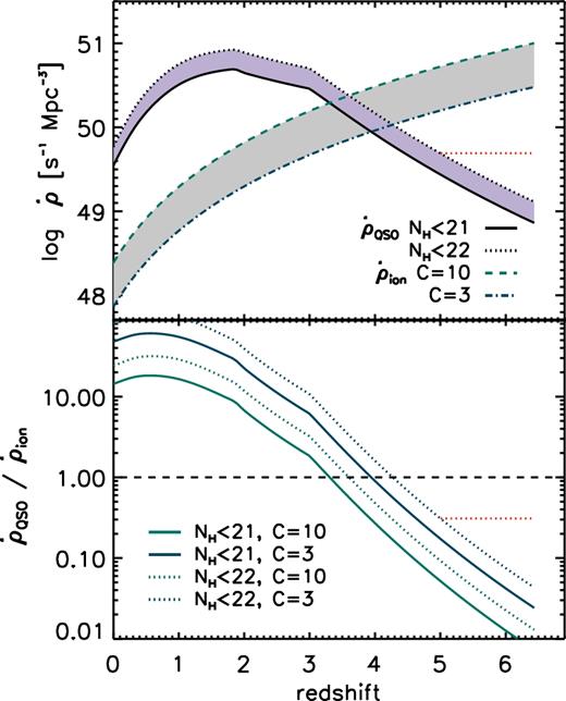
Top: comoving emission rate of hydrogen Lyman continuum photons from QSOs with log NH < 21 cm−2 (black solid line) and with log NH < 22 cm−2 (black dotted line), compared with the minimum rate needed to fully ionize the Universe with clumping factors C = 3, 10 (blue dot–dashed, green dashed lines, respectively). Bottom: contribution of QSO relative to the minimum rate computed with clumping factors C = 3, 10 (blue and green lines, respectively). The dotted red line represents the maximal AGN contribution (see text for details).
The bottom panel in Fig. 4 quantifies the contribution of the X-ray log NH < 21 (solid lines) and log NH < 22 cm−2 (dotted lines) populations relative to the minimum rate obtained from equation (5) using C = 3, 10 (blue and green curves, respectively). At z = 6, redshift of interest for the H i reionization, we find that the contribution of ionizing AGN is little compared to the amount needed to fully ionize the IGM, with a maximum contribution of ∼7 per cent (blue dotted curve; see also Shankar & Mathur 2007, for similar results). If we consider the upper limit at z > 5 on the QSO emissivity, shown in the right-hand panel of Fig. 3, red dotted line (which has been derived under the hypotheses that AGN with log NH < 22 cm−2 contribute significantly to reionization and that the XLF remains constant for z > 5), then the contribution of ionizing AGN increases up to ∼30 per cent (see also Shankar & Mathur 2007). Our results also agree with the very recent findings of Jiang et al. (2016, see their fig. 11) that used a sample of 52 optically selected QSOs at z ∼ 6 in the SDSS to exclude (at 90 per cent confidence, in the case of C = 3) a leading QSO contribution to H i reionization. We note that our best estimate of the AGN ionizing emissivity implies a dominant role of AGN only for z ≲ 4 (see also Georgakakis et al. 2015; Cristiani et al. 2016, and references therein), slightly depending on the choice of the clumping factor C.
6 CONCLUSIONS
The puzzling process of H i reionization and the AGN contribution has been investigated by using complete UV/optically selected QSO and X-ray-selected AGN samples.
In order to better constrain the faint end of the AGN LF at high redshift, we investigated whether the XLF could be used as an unbiased proxy of the ionizing AGN space density. Indeed, X-ray selection offers a better control on the AGN faint end since it is less biased against obscuration. We employed the Ueda et al. (2014) XLF, which is computed in various absorption ranges, to derive a matching between the UV/optical QLF and the X-ray log NH ≲ 21–22 cm−2 AGN LF. The new Chandra COSMOS Legacy Survey z > 3 sample (Marchesi et al. 2016b) is used to validate the extrapolation of Ueda et al. (2014) XLF beyond redshift 5, therefore enabling us to use the 2–10 keV LF of Ueda et al. (2014) to compute the 1 Ryd comoving emissivity up to redshift ∼6. As expected in the traditional AGN unified model framework, when UV/optical data exist we found good agreement between the log NH ≲ 21–22 cm−2 XLF and the optically selected QLF, up to z ∼ 4. This matching implies that the log NH ≲ 21–22 cm−2 XLF can be used as an unbiased proxy to estimate the density of ionizing AGN.
We found that the X-ray log NH < 22 cm−2 LF at z > 4 underpredicts by a factor ∼1 dex the faint end of the UV LF derived using direct UV data. This discrepancy can be attributed to a contribution of UV emission from the AGN host galaxy whose amount is typical of galaxies at break luminosity.
The use of the log NH ≲ 21–22 cm−2 XLFs allows us to measure the 1 Ryd comoving QSO emissivity up to z ∼ 5 without any luminosity extrapolation, extending at ∼5 lower magnitudes than the limits probed by current UV/optical LFs. The evolution of our proposed emissivity with redshift is in agreement also with the functional form proposed by Madau & Haardt (2015) at 0 < z < 2 and with Khaire & Srianand (2015) and Haardt & Madau (2012) at 2 < z < 6 (all derived under different assumptions). At variance, our estimate is smaller at z > 3 than recently found by Madau & Haardt (2015) who proposed an AGN-dominated scenario of H i reionization. We found a high integrated local AGN emissivity as recently proposed by Madau & Haardt (2015).
Finally, we compare the photon emission rate necessary to ionize H i with the critical value needed to keep the Universe ionized, independently of the previous emission history of the Universe. Our findings are that the contribution of ionizing AGN at z = 6 is little, ∼1–7 per cent, with a maximal contribution of ∼30 per cent under the unlikely assumption that the space density of log NH < 22 cm−2 AGN remains constant at z > 5. Our updated ionizing AGN emissivities thus exclude an AGN-dominated scenario at high redshifts, as instead recently suggested by other studies.
While this work makes use of the state of the art in terms of X-ray surveys, at the present day it is impossible to extend this study at redshifts larger than 6. Even in the redshift range 5 < z < 6, the available samples of X-ray-selected high-redshift AGN still suffer from limited statistics, and are biased against relatively low luminosities (L2-10 keV ≤ 1043 erg s−1; below the LF break). Only future facilities, like Athena (Nandra et al. 2013) and the X-raySurveyor (Vikhlinin 2015), will be able to collect sizable samples (∼100s) of low-luminosity (L2-10 keV < 1043 erg s−1) AGN at z > 5 (Civano 2015).
Acknowledgments
We thank F. Fiore, F. Fontanot, E. Giallongo, A. Grazian and M. Volonteri for useful discussions. We thank the anonymous referee for her/his valuable comments that improved the quality of the manuscript. We acknowledge funding from PRIN/MIUR-2010 award 2010NHBSBE and PRIN/INAF. This work was partially supported by NASA Chandra grant numbers GO3-14150C and GO3-14150B (FC, SM).
We adapted their QLF to our adopted cosmology.
This XLF has been convolved with a 0.4 dex Gaussian scatter, as already described in Section 3.1.
The Vega absolute B magnitude MB were converted into B-band luminosity LB in a similar way as in equation (3) (substituting the magnitudes and luminosities) with f0 = 4.063 × 10⁻²⁰ erg s−1 cm−2 Hz−1. Finally, LB was translated into L912 with our adopted SED (see Section 3). The integration limit used was log Lmin = 29.42 erg s−1 Hz−1. The uncertainties on this local emissivity have been evaluated directly from the uncertainties on the binned QLF.
The photon underproduction crisis is the finding of Kollmeier et al. (2014) of a five times higher H i photoionization rate (|$\Gamma _{\rm H\,\small {i}}$|) at z = 0, obtained matching the observed properties of the low-redshift Ly α forest (such as the Ly α flux decrement and the bivariate column density distribution of the Ly α forest; e.g. Danforth et al. 2016), than predicted by simulations which include state-of-the art models for the evolution of the UVB (e.g. Haardt & Madau 2012). A similar investigation was carried out also by Shull et al. (2015), who found a lower discrepancy (i.e. only a factor ∼2 higher) with the UVB model of Haardt & Madau (2012).
