


Abstract
We derive new empirical calibrations for strong-line diagnostics of gas-phase metallicity in local star-forming galaxies by uniformly applying the Te method over the full metallicity range probed by the Sloan Digital Sky Survey (SDSS). To measure electron temperatures at high metallicity, where the auroral lines needed are not detected in single galaxies, we stacked spectra of more than 110 000 galaxies from the SDSS in bins of log[O ii]/Hβ and log[O iii]/Hβ. This stacking scheme does not assume any dependence of metallicity on mass or star formation rate, but only that galaxies with the same line ratios have the same oxygen abundance. We provide calibrations which span more than 1 dex in metallicity and are entirely defined on a consistent absolute Te metallicity scale for galaxies. We apply our calibrations to the SDSS sample and find that they provide consistent metallicity estimates to within 0.05 dex.
1 INTRODUCTION
The accurate determination of gas-phase metallicity represents a challenging topic for studies that aim at understanding the chemical evolution of galaxies. The metal content of a galaxy is regulated by complex interactions between physical processes occurring on different spatial and time-scales: heavy elements produced by stellar activity contribute to the enrichment of the interstellar medium (ISM), while cosmological infall of pristine gas from the intergalactic medium (IGM) and outflows due to active galactic nuclei (AGN) and supernovae could dilute the ISM and at the same time trigger new star formation episodes (Davé, Finlator & Oppenheimer 2011). These processes directly impact the global baryon cycle and thus affect other physical quantities strictly related to the history of chemical enrichment in galaxies like stellar mass (M⋆) and star formation rate (SFR); therefore, relationships between these parameters and gas-phase metallicity are expected. Indeed, in the last decades strong observational evidences of a correlation between M⋆ and gas-phase metallicity (the so-called mass–metallicity relation, M–Z) have been reported by several studies, both in the local Universe (e.g. Tremonti et al. 2004; Lee et al. 2006; Liang et al. 2007) and at higher redshift, where signatures of a cosmic evolution have been found (e.g. Erb et al. 2006; Maiolino et al. 2008; Mannucci et al. 2009; Cresci et al. 2012; Zahid et al. 2012; Troncoso et al. 2014). Furthermore, Mannucci et al. (2010) showed that the intrinsic scatter in the M–Z could be reduced when SFR is taken into account, introducing the concept of a fundamental metallicity relation (FMR) that reduces the M–Z to a two-dimensional projection of a three-dimensional surface. The FMR appears to be more fundamental in the sense that it does not seem to present clear signs of evolution up to z ∼ 2.5. Even though the physical origin of these relations is still debated, the knowledge of the main properties of the M–Z and the exact form of its dependence upon the SFR is important to investigate the processes regulating star formation and to assess the role of outflows in ejecting metals out of the galaxy (Davé, Finlator & Oppenheimer 2011; Dayal, Ferrara & Dunlop 2013; Lilly et al. 2013); this could provide crucial observational constraints for models aimed at reproducing the chemical evolution of galaxies across cosmic time.
Investigating the properties of these relationships and their redshift evolution requires precise and robust metallicity estimates. Since the scatter in the FMR is of the order of 0.05 dex (Mannucci et al. 2010), such a level of precision in metallicity determination would be desirable. There are several ways to measure abundances in galaxies, but unfortunately none of them is considered reliable or applicable over the whole metallicity range covered by large galaxy samples. The most commonly used method relies on the determination of the electron temperature of the nebulae responsible for emission lines in galaxies: in fact, electron temperature is known to be strongly correlated with metallicity, such that higher metallicities are associated with lower Te, because forbidden emission lines from metals are the primary coolants in H ii regions. Electron temperatures can be inferred by exploiting the temperature sensitive auroral to nebular line ratios of particular ions (e.g. [O iii] λ4363/5007 is one of the most widely used); in fact, the atomic structure of these ions is such that auroral and nebular lines originate from excited states that are well spaced in energy and thus their relative level populations depend heavily on electron temperature. This so-called Te method is widely accepted as the preferred one to estimate abundances since it is a direct probe of the processes that regulate the physics of ionized nebulae. Unfortunately, auroral lines are weak in most of individual galaxy spectra, especially for metal-rich objects, which typically prevents the Te from being used as a method to determine abundances of metal-enriched galaxies. A different technique is based instead on exploiting the ratio between oxygen and hydrogen recombination lines (RLs): since these lines show a very weak dependence on electron temperature and density (Esteban et al. 2009, 2014; Peimbert & Peimbert 2014), this is probably the most reliable method because it is unaffected by the typical biases of the Te method associated with temperature fluctuations. Typical discrepancies between Te- and RLs-based abundances are found to be of the order of 0.2–0.3 dex, with the first ones underestimating the latter (García-Rojas & Esteban 2007; Esteban et al. 2009). Recently, Bresolin et al. (2016) showed that metal RLs yield nebular abundances in excellent agreement with stellar abundances for high-metallicity systems, while in more metal-poor environments they tend to underestimate the stellar metallicities by a significant amount. However, RLs are extremely faint (even hundred times fainter than oxygen auroral lines) and cannot be detected in galaxies more distant than a few kiloparsecs (Peimbert et al. 2007). For this reason, different methods have been developed to measure abundances in faint, distant and high-metallicity galaxies. In particular, it is known that some line ratios between strong collisionally excited lines (CELs) and Balmer lines show a dependence on metallicity, which can be either directly motivated or indirectly related to other physical quantities (e.g. the ionization parameter). Thus, it has been proposed that these line ratios could be calibrated against the oxygen abundance and used as metallicity indicators for galaxies in which the application of the Te method is not possible due to the extreme faintness of auroral lines (Alloin et al. 1979; Pagel et al. 1979): these are referred to as the strong-line methods. Calibrations can be obtained either empirically, for samples in which metallicity have been previously derived with the Te method (e.g. Pettini & Pagel 2004; Pilyugin & Thuan 2005; Pilyugin, Vílchez & Thuan 2010b; Pilyugin, Grebel & Mattsson 2012; Marino et al. 2013; Pilyugin & Grebel 2016), or theoretically, in which oxygen abundance have been inferred via photoionization models (e.g. McGaugh 1991; Zaritsky, Kennicutt & Huchra 1994; Kewley & Dopita 2002; Kobulnicky & Kewley 2004; Tremonti et al. 2004; Dopita et al. 2013, 2016), or be a combination of the two. Unfortunately, comparisons among metallicities estimated through different calibrations reveal large discrepancies, even for the same sample of objects, with variations up to ∼0.6 dex (Kewley & Ellison 2008; Moustakas et al. 2010). In fact, theoretical calibrations are known to produce higher metallicity estimates with respect to empirical calibrations based on the Te method. The origin of these discrepancies is still unclear, but they could be attributed on one hand to oversimplified assumptions made in most of the photoionization models, e.g. about the geometry of the nebulae and the age of the ionizing source (Moustakas et al. 2010) and on the other hand to temperature gradients and fluctuations that may cause an overestimate of the electron temperature and a consequent underestimate of the true metallicity with the Te method (Peimbert 1967; Stasińska 2002, 2005). Great care is therefore needed when using composite calibrations built with different methods over different metallicity ranges, due to the large uncertainties introduced on the absolute metallicity scale. Empirical calibrations are generally preferable because they are based on the Te method abundance scale, which is directly inferred from observed quantities. Moreover, on the abundance scale based on photoionization models, the Milky Way, where abundances can be precisely measured, would represent a very peculiar galaxy, falling well below the M–Z defined by similar star-forming galaxies. The discrepancy is reduced by more empirical metallicity calibrations that provide lower abundances. At the same time, one of their main limitations is that they are often calibrated for samples of objects that do not properly cover all the galaxy parameters space; this means, for example, that empirical calibrations obtained from a sample of low excitation H ii regions could give unreliable results when applied to global galaxy spectra. Recently, the application of integral field spectroscopy allowed to study galaxy properties in great detail and to extend the H ii regions data base for compiling abundances in order to obtain calibrations based on the Te method [e.g. Marino et al. 2013 for the Calar Alto Legacy Integral Field Area (CALIFA) survey]. However, self-consistent calibrations obtained from integrated galaxy spectra and covering the entire metallicity range are still scarce.
In this work we derive a set of new empirical calibrations for some of the most common strong-line metallicity indicators, thanks to a uniform application of the Te method over the full metallicity range covered by Sloan Digital Sky Survey (SDSS) galaxies. We combined a sample of low-metallicity galaxies with [O iii] λ4363 detection from the SDSS together with stacked spectra of more than 110 000 galaxies in bins of log[O ii]/Hβ–log[O iii]/Hβ that allowed us to detect and measure the flux of the crucial auroral lines needed for the application of the Te method also at high metallicity. Other studies demonstrated the potentiality and reliability of the stacking technique (Liang et al. 2007; Andrews & Martini 2013; Brown, Martini & Andrews 2016); compared to these works, our approach differs in the sense that we do not rely on any assumption regarding the nature and the form of the relationships between metallicity, mass and SFR, but only on the hypothesis that oxygen abundance can be determined from a combination of [O ii] and [O iii] emission line ratios.
The paper is organized as follows. In Section 2 we describe the sample selection and the procedure used to stack the spectra, subtract the stellar continuum and fit the emission lines of interest. Section 3 describes the method we used to derive electron temperatures and chemical abundances. We then discuss the relations between different temperature diagnostics and between temperatures of different ionization zones. In Section 4 we report some tests we performed to verify the consistency of our hypothesis and stacking procedure. In Section 5, we present our new empirical calibrations for some of the most common strong-line abundance diagnostics and we compare them with previous ones from literature. We then apply them to the original SDSS sample as a test of their self-consistency. Section 6 summarizes our main results.
Publicly available tools to apply these new calibrations can be found on the web page http://www.arcetri.astro.it/metallicity/.
2 METHOD
2.1 Sample selection
Our galaxy sample comes from the SDSS Data Release 7 (DR7; Abazajian et al. 2009), a survey including ∼930 000 galaxies in an area of 8423 deg2. Emission line data have been taken from the MPA/JHU1 catalogue, in which also stellar masses (Kauffmann et al. 2003a), SFRs (Brinchmann et al. 2004; Salim et al. 2007) and metallicities (Tremonti et al. 2004) are measured. We chose only galaxies with redshifts in the range 0.027 < z < 0.25, to ensure the presence of the [O ii] λ3727 emission line and of the [O ii] λλ7320, 7330 doublet within the useful spectral range of the SDSS spectrograph (3800–9200 Å). We selected only galaxies classified in the MPA/JHU as star forming, discarding galaxies dominated by AGN contribution according to criteria for BPT-diagram classification illustrated in Kauffmann et al. (2003b), in order to avoid any effect on the emission line ratios that could cause spurious metallicity measurements. We also used a signal-to-noise ratio (S/N) threshold of 5 on the Hα, Hβ, [O iii] λ5007 and [O ii] λ3727 emission line fluxes. After applying these selection criteria, the total number of galaxies in our sample was reduced to 118 478, with a median redshift of z = 0.072. At this redshift, the 3 arcsec diameter of the SDSS spectroscopic fibre corresponds to ∼3 kpc.
2.2 Stacking procedure
Our primary goal is to perform accurate measurements of galaxy metallicity in order to obtain more consistent calibrations for the main strong-line indicators, thanks to a uniform application of the Te method. Unfortunately, in distant galaxies the [O iii] λ4363 and [O ii] λλ7320, 7330 auroral lines are too weak to be detected in the individual spectra at metallicities higher than 12 + log(O/H) ≳ 8.3. Thus, we decided to stack spectra for galaxies that are expected to have similar metallicities.
Galaxies are stacked according to their values of reddening corrected [O ii]λ3727/Hβ and [O iii]λ5007/Hβ flux ratios. This is based on the assumption that the so-called strong-line methods can be used to discriminate the metallicities of star-forming galaxies when multiple line ratios are simultaneously considered. We stress that we are not assuming that a particular combination of these line ratios, such as R23, is related to metallicity, but only that galaxies with simultaneously the same values of both [O iii]λ5007/Hβ and [O ii]λ5007/Hβ have approximately the same oxygen abundance. In fact, these are the two line ratios directly proportional to the main ionization states of oxygen and are thus individually used as metallicity diagnostics (Nagao, Maiolino & Marconi 2006; Maiolino et al. 2008). Moreover, their ratio [O iii]/[O ii] is sensitive to the ionization parameter and it is also used as an indicator of oxygen abundance, especially in metal-enriched galaxies, due to the physical link between ionization and gas-phase metallicity (e.g. Nagao et al. 2006; Masters, Faisst & Capak 2016). This means that the location of a galaxy on the [O ii]λ3727/Hβ–[O iii]λ5007/Hβ diagram is primarily driven by the metal content and the ionization properties of galaxies. Since the scatter in a given line ratio at fixed metallicity is often regarded as driven by variations in the ionization parameter (e.g. Kewley & Dopita 2002; López-Sánchez et al. 2012; Blanc et al. 2015) our binning choice takes into account this possible source of scatter.
The left-hand panel of Fig. 1 shows the distribution of our selected SDSS galaxies in the log [O ii]λ3727/Hβ–log [O iii]λ5007/Hβ diagnostic diagram. We overplot the semi-empirical calibration of Maiolino et al. (2008) for the [O ii]λ5007/Hβ and [O iii]λ5007/Hβ indicators in order to better visualize how the position on the 2D diagram given by the combination of these line ratios represent a metallicity sequence. The curve, colour coded for the metallicity inferred from the combination of the two indicators, follows quite tightly the distribution of galaxies on the map, showing how metallicity increases from the upper left region of the diagram to the bottom left one. To further illustrate how metallicity varies along this diagram, we can also use the metallicity obtained with the Te method from composite spectra in bins of stellar mass by Andrews & Martini (2013), whose stacks are shown as circled points in the left-hand panel of the figure. Also in this case we can recognize a pattern in which their mass stacks, each point being representative of the line ratios measured from the associated composite spectra, increase monotonically in metallicity following the galaxy sequence on the diagram. Thus, both methods reveal a clean variation of oxygen abundance with location on the diagram, though being based on different and independent approaches; this strengthens the idea of using the combination of [O ii]/Hβ and [O iii]/Hβ as a metallicity indicator. We note that differences among metallicity values predicted by the Maiolino et al. (2008) calibrations and the Andrews & Martini (2013) stacks (with the first ones predicting higher abundances than the latter) are only due to the different abundance scale upon which the two methods are defined, being the Maiolino et al. (2008) indicators calibrated with photoionization models at high metallicities and the Andrews & Martini (2013) stacks based on Te method metallicities.
![Left-hand panel: the distribution of our galaxy sample in the log [O ii] λ3727/Hβ–log [O iii] λ5007/Hβ diagram. The curve represents the combined calibrations for the [O ii]/Hβ and [O iii]/Hβ metallicity indicators from Maiolino et al. (2008), colour coded by the metallicity inferred from the combination of the two indicators. The Andrews & Martini (2013) stacks in bins of stellar mass are shown as circle points and colour coded for their direct metallicity measurement. Right-hand panel: stacking grid for our sample of SDSS galaxies in the log [O ii] λ3727/Hβ–log [O iii] λ5007/Hβ diagram. Each square represents a 0.1 × 0.1 dex2 bin, colour coded by the number of galaxies included in it, which is also written for each bin. Orange boxes represent stacks of low-metallicity galaxies for which we relaxed the 100-object threshold in the definition of our grid. In the upper right box of the panel our stacking grid is shown superimposed on the distribution of galaxies in the diagram.](https://oup.silverchair-cdn.com/oup/backfile/Content_public/Journal/mnras/465/2/10.1093_mnras_stw2766/3/m_stw2766fig1.jpeg?Expires=1750229202&Signature=CcqrfdEkcdJ7O1iKp0cvnVepp5S0YCNlDdVA~i7h19aXyCWbiBtO9IxUXhgTlawL0tcdlZU9N0U4~VZGRNK6dukguoGtct3hRhYqN7ZnZQFq-M9bunHIMvrS7mpZwtw6c~gGXMq9anvmfQq6bMZ317iPI0OjJ14hVhBFdxgdDTgmQBfWI4Fh7yoMKtOzlgDmrtlF~l9QDJYGbKXEKB0zeooDRR1BbfIwcnga50UedbDqPiSvbtN~1do~~Csq8yka1zYbsqVHCm9qI5YYm-yHwbR3AChKi7tTeo4KyiFQZORhKOuR5MgYwVPzQW3pk0cR3A39ChlBDUELv1vVCRMKMQ__&Key-Pair-Id=APKAIE5G5CRDK6RD3PGA)
Left-hand panel: the distribution of our galaxy sample in the log [O ii] λ3727/Hβ–log [O iii] λ5007/Hβ diagram. The curve represents the combined calibrations for the [O ii]/Hβ and [O iii]/Hβ metallicity indicators from Maiolino et al. (2008), colour coded by the metallicity inferred from the combination of the two indicators. The Andrews & Martini (2013) stacks in bins of stellar mass are shown as circle points and colour coded for their direct metallicity measurement. Right-hand panel: stacking grid for our sample of SDSS galaxies in the log [O ii] λ3727/Hβ–log [O iii] λ5007/Hβ diagram. Each square represents a 0.1 × 0.1 dex2 bin, colour coded by the number of galaxies included in it, which is also written for each bin. Orange boxes represent stacks of low-metallicity galaxies for which we relaxed the 100-object threshold in the definition of our grid. In the upper right box of the panel our stacking grid is shown superimposed on the distribution of galaxies in the diagram.
In Section 4 we test our assumptions by comparing Te metallicities inferred from single galaxy spectra belonging to the same bin; this allows also to evaluate the main issues related to the stacking technique (see also the discussion in Section 3.2). We refer to these sections for an exhaustive discussion on this topic.
We thus created stacked spectra in bins of 0.1 dex of log [O ii]/Hβ and log [O iii]/Hβ. The choice of the 0.1 dex width in the binning grid represents a good compromise between keeping a high enough number of galaxy in each bin to ensure auroral line detection and at the same time avoid wider bins in which we could have mixed objects with too different properties. We performed some tests in stacking spectra and computing oxygen abundance with different bin sizes, finding no relevant differences.
We adopted the emission line values provided by the MPA/JHU catalogue to create the set of galaxy stacks. All line fluxes have been corrected for Galactic reddening, adopting the extinction law from Cardelli, Clayton & Mathis (1989) and assuming an intrinsic ratio for the Balmer lines Hα/Hβ = 2.86 (as set by case B recombination theory for typical nebular temperatures of Te = 10 000 K and densities of ne ≈ 100 cm−3).
In the right-hand panel of Fig. 1, the binning grid for our galaxy sample in the space defined by log([O ii] λ3727/Hβ) and log([O iii] λ5007/Hβ) is shown, colour coded by the number of objects in each bin. In the upper right-hand corner of the figure we show the distribution of the galaxy sample in the diagnostic diagram, with our binning grid superimposed. In the construction of our binning grid we required a minimum of 100 sources per bin: this was a conservative choice in order to average enough galaxy spectra to ensure the required S/N (i.e. at least 3) on auroral line detection after the stacking procedure. Since we imposed a threshold of 100 sources per bin, the upper left-hand corner of the diagram, occupied by the galaxies of lower metallicity in the sample, is not well covered by our stacking grid. For this reason, we extended our grid to include also low-metallicity galaxies by reducing the threshold to 10 sources in that area of the diagram, enough to detect auroral lines in stacked spectra with an S/N higher than 3 in this metallicity regime. This extension of the grid is marked with orange borders in the figure. This allows our grid to entirely cover the region occupied by SDSS galaxies, probing the largest possible combination of physical parameters in the sample. Throughout this paper we will refer to a particular stack by indicating the centre of the corresponding bin in both the line ratios considered (e.g. 0.5; 0.2 corresponds to the bin centred in log[O ii] λ3727/Hβ = 0.5 and log[O iii] λ5007/Hβ = 0.2).
Before creating the composite spectrum from galaxies belonging to the same bin, each individual spectrum has been corrected for reddening with a Cardelli et al. (1989) extinction law and normalized to the extinction corrected Hβ. We have verified that the final results do not depend on the choice of the extinction law, by alternatively using the Calzetti, Kinney & Storchi-Bergmann (1994) extinction law in a few random bins. Then, each spectrum has been re-mapped on to a linear grid (3000–9200 Å), with wavelength steps of Δλ = 0.8 Å, and shifted at the same time to the rest frame to compensate for the intrinsic redshift of the sources. This procedure may cause a redistribution of the flux contained in a single input channel to more than one output channel; in order to take into account this effect, the incoming flux is weighted on the overlap area between the input and output channels. Finally, to create the stacked spectra we took the mean pixel by pixel between the 25th and the 75th percentile of the flux distribution in each wavelength bin; in this way we could avoid biases introduced by the flux distribution asymmetry clearly visible in every flux channel as a right-end tail.
2.3 Stellar continuum subtraction
Stacking the spectra improves significantly the S/N of the auroral lines, but we must also fit and subtract the stellar continuum to accurately measure their fluxes. To perform the stellar continuum fit and subtraction on our stacked spectra, we have created a synthetic spectrum using the MIUSCAT library of spectral templates (Ricciardelli et al. 2012; Vazdekis et al. 2012), an extension of the previous MILES library (Cenarro et al. 2001; Sánchez-Blázquez et al. 2006; Vazdekis et al. 2010; Falcón-Barroso et al. 2011) in which both Indo-US and CaT libraries have been added to fill the gaps in wavelength coverage. The new MIUSCAT library covers a wavelength range of 3525–9469 Å, although the useful spectral window for this work is entirely covered by MILES templates, whose resolution is 2.51 Å [full width at half-maximum (FWHM)]. Stellar templates have been retrieved from the MILES web site2 for a wide range of ages and metallicities, assuming a unimodal initial mass function (IMF) with a 1.3 slope (i.e. a Salpeter IMF). The stellar continuum subtraction in the [S ii] λ4069 spectral window (close to Hδ) has been performed using a different kind of stellar templates, the PÉGASE HR3 (Le Borgne et al. 2004), a library which covers a wavelength range of 4000–6800 Å with a spectral resolution of R = 10 000 at λ = 5500 Å; this allowed a better stellar continuum fit in the proximity of the [S ii] λ4069 auroral line. To further improve emission line fluxes measurements, stellar continuum fits and subtractions have been performed selecting subregions of the spectrum centred on the lines of interest, each subregion being large a few hundred angstrom. During the procedure the location of the emission lines has been masked out in order to prevent the fit to be affected by non-stellar features. We performed the fit exploiting the idl version of the penalized pixel-fitting (ppxf) procedure by Cappellari & Emsellem (2004). In Table 1 is reported, for each emission lines whose flux have been measured in this work, the spectral window of the stellar continuum fit and the wavelength range that has been masked out. Fig. 2 shows examples of the results of the stacking procedure and stellar continuum subtraction for the 0.5; 0.5 bin, in particular in spectral windows including Hβ, [O iii] , Hα, [N ii] and [S ii] nebular lines and [O iii] λ4363, [O ii] λλ7320, 7330 auroral lines, respectively. For latter emission lines, a single galaxy spectrum from the same stack is shown for comparison, to underline the dramatic increase in S/N that allows to reveal the otherwise invisible auroral lines. The orange regions mark the spectral range masked out from the stellar fitting around nebular lines. In each plot, the lower panel shows the residual spectrum of the fit.
![Fit and subtracted spectra for wavelength ranges relative to Hβ and [O iii] nebular lines (upper left-hand panels), Hα, [N ii] and [S ii] nebular lines (upper right-hand panels), [O iii] λ4363 auroral line (lower left-hand panels) and [O ii] λλ7320, 7330 auroral lines (lower right-hand panels), respectively, for the 0.5; 0.5 stack. For strong nebular lines, the upper panel shows the stacked spectrum (black) and the stellar continuum best-fitting component (red), while the bottom panel shows the residual spectrum after the stellar continuum subtraction. For auroral line boxes, a single galaxy spectrum is shown in the upper panel for comparison, while the stacked spectrum is shown in the middle one. The yellow shaded regions mark the spectral interval masked out during the stellar continuum fitting procedure.](https://oup.silverchair-cdn.com/oup/backfile/Content_public/Journal/mnras/465/2/10.1093_mnras_stw2766/3/m_stw2766fig2.jpeg?Expires=1750229202&Signature=42wtLr5OFLDswapnVBv2NA58ixY82UPBR8Z0z-9A0CH9xOyqjXslCOTIfNfErT6obD2hoIhCAv38P01wZzCCM-5hDy2HEKd3zcc-TZdnPKt~M3PuKL~mZocmb3KxeQkrFZoNbcRSG0W6BptkQMDJMCD75BSuqv63r2CCqTCe8~fG-BwZftB~t4XNyM~hilqKFXzvo1DCeQZpz7x26pnVD5xzAinT3TGgSFECxIMdDSYEhT5lOuuwJ9fiXQ-z5uG0DmzmetY57KI2hYAw3y~YnpvG0Hg1qf79FSUKSuOcoHWAMz701v~CaQT0I3cdbJ40BMgAkHURD7aUW7fc0oW8Yw__&Key-Pair-Id=APKAIE5G5CRDK6RD3PGA)
Fit and subtracted spectra for wavelength ranges relative to Hβ and [O iii] nebular lines (upper left-hand panels), Hα, [N ii] and [S ii] nebular lines (upper right-hand panels), [O iii] λ4363 auroral line (lower left-hand panels) and [O ii] λλ7320, 7330 auroral lines (lower right-hand panels), respectively, for the 0.5; 0.5 stack. For strong nebular lines, the upper panel shows the stacked spectrum (black) and the stellar continuum best-fitting component (red), while the bottom panel shows the residual spectrum after the stellar continuum subtraction. For auroral line boxes, a single galaxy spectrum is shown in the upper panel for comparison, while the stacked spectrum is shown in the middle one. The yellow shaded regions mark the spectral interval masked out during the stellar continuum fitting procedure.
Spectral windows and mask ranges of measured emission lines. Column (1): emission lines; column (2): wavelength range of stellar continuum fit; column (3): spectral range that was masked out.
| Line | Fit range | Mask range |
|---|---|---|
| (Å) | (Å) | |
| (1) | (2) | (3) |
| [O ii] λ3727 | 3650–3830 | 3723.36–3733.60 |
| [Ne iii] λ3870 | 3850–4150 | 3866.29–3874.03 |
| [S ii] λ4069 | 4000–4150 | 4068.39–4071.11 |
| Hδ λ4102 | 3850–4150 | 4098.79–4107.00 |
| Hγ λ4340 | 4250–4450 | 4337.34–4346.03 |
| [O iii] λ4363 | 4250–4450 | 4362.98–4365.89 |
| Hβ λ4861 | 4750–5050 | 4857.82–4867.55 |
| [O iii] λ4960 | 4750–5050 | 4955.33–4965.26 |
| [O iii] λ5007 | 4750–5050 | 5003.23–5013.25 |
| [N ii] λ5756 | 5650–5850 | 5754.32–5758.16 |
| [N ii] λ6549 | 6480–6800 | 6543.30–6556.40 |
| Hα λ6563 | 6480–6800 | 6558.05–6571.17 |
| [N ii] λ6584 | 6480–6800 | 6578.69–6591.87 |
| [S ii] λ6717 | 6480–6800 | 6711.57–6725.01 |
| [S ii] λ6731 | 6480–6800 | 6725.94–6739.40 |
| [O ii] λ7320 | 7160–7360 | 7318.50–7323.28 |
| [O ii] λ7330 | 7160–7360 | 7329.24–7334.12 |
2.4 Line flux measurement and iron contamination of [O iii] |$\boldsymbol {\lambda 4363}$| auroral line at high metallicity
We fit emission lines with a single Gaussian profile, fixing velocities and widths of the weak auroral lines by linking them to the strongest line of the same spectral region. For doublets, we fixed the velocity width of the weaker lines to the stronger ones ([O ii] λ3727 to [O ii] λ3729, [O iii] λ4960 to [O iii] λ5007, [N ii] λ6548 to [N ii] λ6583, [S ii] λ6731 to [S ii] λ6717 and [O ii] λ7330 to [O ii] λ7320).
During the fitting procedure, an emission feature close to 4360 Å has been detected and become blended with the [O iii] λ4363 auroral line, especially in the high-metallicity stacks. A similar contamination was previously found also by Andrews & Martini (2013) in their composite spectra. The nature of this feature is unknown, but it may reasonably be associated with emission lines from [Fe ii] λ4360. In fact, many others features from the same ion are clearly observable both in the same (e.g. [Fe ii] λ4288) and in different spectral windows; this particular emission has been reported also in studies on the Orion nebula (see e.g. table 2 of Esteban et al. 2004). Moreover, the strength of the line increases with increasing metallicity, as well as the other [Fe ii] lines in the spectra. In Fig. 3 we show three stacked spectra corresponding to different metallicities, namely 0.4; 0.6, 0.5; 0.0 and 0.2; −0.6, after performing the stellar continuum subtraction in the spectral window that contains the [O iii] λ4363 line. The metallicity of each stack (see Section 5) is reported on every panel. The figure clearly shows how [O iii] λ4363 becomes more contaminated as the metallicity increases, with the [Fe ii] emission being just a few per cent of the flux of the oxygen one in the upper panel and then completely blending with it in the other two. The [Fe ii] emission line at 4288 Å is also clearly visible in all the composite spectra, with increasing strength for increasing metallicity, as expected.
![Left: composite spectra for the 0.4; 0.6 (upper panel), 0.5; 0.0 (middle panel) and 0.2; −0.6 (lower panel) stack, in the wavelength range relative to [O iii] λ4363, after the stellar continuum subtraction. The different components of the fit are reported in blue while the red curve represents the total fit. The metallicity of each stack is reported in the right-upper part of the corresponding panel. The contamination of the [O iii] λ4363 line becomes more relevant with increasing metallicity (in the last case we can fit up to three components), as well as the intensity of the [Fe ii] emission line at 4288 Å.](https://oup.silverchair-cdn.com/oup/backfile/Content_public/Journal/mnras/465/2/10.1093_mnras_stw2766/3/m_stw2766fig3.jpeg?Expires=1750229202&Signature=lPqe1kGNpiyDZplK9K673FlEmkoNWpt0nADpXyxFC~CxEoCU-M3RHGhyVfMueh2CcmoKHjvjzPqadsGEbY1ywk9K9UNLau1P1HxYe5Yx3BJCIB2SACZqmaOaoZhxN~WCWqJGv~IwTHRas6XotjkdtXotTcrG5tsbZf9rDwVIT0xkiBO-aMmtXyof1WGOSaqSqT1RoNKSLpdswyDmngH-JUlvRv8bqB9e7rWb~UEZLusOx16Jpo-0y00kXrYrtpfhRX6TIcuigrTngiq5mkCdRDoDsbSoGVrv2fWKDhhi47kBhvF02pVaUaX8fPDVjbXhnMXWwM1cYzIaB1SV4PCHRA__&Key-Pair-Id=APKAIE5G5CRDK6RD3PGA)
Left: composite spectra for the 0.4; 0.6 (upper panel), 0.5; 0.0 (middle panel) and 0.2; −0.6 (lower panel) stack, in the wavelength range relative to [O iii] λ4363, after the stellar continuum subtraction. The different components of the fit are reported in blue while the red curve represents the total fit. The metallicity of each stack is reported in the right-upper part of the corresponding panel. The contamination of the [O iii] λ4363 line becomes more relevant with increasing metallicity (in the last case we can fit up to three components), as well as the intensity of the [Fe ii] emission line at 4288 Å.
Therefore we simultaneously fit the λ4360 feature and [O iii] λ4363, linking both velocity widths and central wavelengths to Hγ. The different components of the fit are shown in blue in Fig. 3, with the red line representing the total fit. Similarly to Andrews & Martini (2013), we consider the fit not sufficiently robust when the λ4360 emission flux resulted ≥0.5 times the flux measured for [O iii] λ4363. The use of contaminated [O iii] λ4363 line would result in totally non-physical temperatures, which result overestimated by a factor of 10. According to this criterion, 42 out of 69 bins have been flagged for undetected [O iii] λ4363. We note that many previous detection of the [O iii] λ4363 may be possibly contaminated by this feature, resulting in unreliable measurements for this crucial auroral line; therefore, we recommend great care in using [O iii] λ4363, when detected, to measure electron temperature from high metallicity (12+log(O/H) ≥ 8.3) galaxy spectra. In the next section we discuss how to derive the electron temperature for the high-ionization zone for those stacks where the [O iii] λ4363 was not considered sufficiently robust.
Despite the large number of galaxies in each bin and the great care in the fitting procedure, in some of our stacks we were unable to measure both [O ii] and [O iii] auroral line fluxes with sufficient precision. These are the stacked spectra corresponding to the 0.0; −0.8, 0.1; −0.4, 0.1; −0.7, 0.1; −0.8, 0.8; 0.2 and 0.6; −0.3 bins and we decided to exclude this stacks from all the forthcoming analysis.
3 ELECTRON TEMPERATURES AND IONIC ABUNDANCES DETERMINATION
3.1 Electron temperatures
In principle, to measure electron temperatures and densities of different zones, the complete ionization structure of a H ii region is needed. This is actually not possible and simpler approximations are always used. Usually a two-zone (of low and high ionization) or even a three-zone (of low, intermediate and high ionization) structure is adopted to model the H ii regions responsible for emission lines in galaxies. In this work we consider a two-zone H ii region: in this scenario, the high-ionization zone is traced by the O++ ion, while the low-ionization zone could be traced by different ionic species, e.g. O+, N+ and S+. Thus, given the SDSS spectral coverage, in our case we have three different diagnostics for the temperature of the low-ionization zone (which we will refer to as t2 from now on), namely [O ii] λλ3727, 3729/[O ii] λλ7320, 7330, [N ii] λ6584/[N ii] λ5755 and [S ii] λλ6717, 6731/[S ii] λ4969, but only one for the temperature of the high-ionization zone (t3), namely [O iii] λ5007/[O iii] λ4363. Other collisionally excited lines probing the temperature of the intermediate- and high-ionization region are either too weak and thus undetectable even in galaxy stacks (e.g. [Ar iii] λ5192) or fall outside the spectral range of the SDSS spectrograph (e.g. [S iii] λ9069, [Ne iii] λ3342) and we could not use them.
We computed electron temperatures exploiting PyNeb (Luridiana, Morisset & Shaw 2012, 2015), the python-based version of the stsdas nebular routines in iraf, using the new atomic data set presented in Palay et al. (2012). These routines, which are based on the solution of a five-level atomic structure following De Robertis, Dufour & Hunt (1987), determine the electron temperature of a given ionized state from the nebular to auroral flux ratio assuming a value for electron density. The electron density ne can be measured from the density sensitive [S ii] λλ6717, 6731 or [O ii] λλ3727, 3729 doublets. In the majority of our stacks we fall in the low-density regime (ne < 100 cm−3), for we measure for example a [S ii] ratio close to the theoretical limit of 1.41; in this case the dependence of our temperature diagnostics upon density is small. We note that using older atomic data sets (e.g. Aggarwal & Keenan 1999), instead on the new ones by Palay et al. (2012), would result in similar t2 but t3 systematically higher on average by 400 K. This is consistent with expectations given the updated effective collision strengths for [O iii] lines, as pointed out e.g. in Nicholls et al. (2013) where a discrepancy of ∼500 K is expected at T[O iii] ∼104 K (see e.g. section 7 and figs 2 and 12 of their paper for further details). We also note that the collision strengths presented in Palay et al. (2012) for the [O iii] optical transitions are tabulated for a wide range of temperatures typical of nebular environments (from 100 to 30 000 K), which include all the temperatures we expect to find given the metallicity range spanned by the SDSS galaxies. Temperatures uncertainties were computed with Monte Carlo simulations. We generated 1000 realizations of the flux ratios, following a normal distribution with σ equal to the errors associated with the flux measurement by the fitting procedure and propagated analytically, and for each of them a temperature value was calculated. Then, we took the standard deviation of the resulting distribution as the error to associate to our temperature measure.
The left-hand panels of Fig. 4 show the relations between the temperatures of the low-ionization zone of our stacks inferred through different diagnostics, i.e. Te[N ii] (upper panel) and Te[S ii] (lower panel) as a function of Te[O ii]; the black line represents the line of equality. In the upper panel, we can see how the electron temperatures derived from nitrogen line ratios are consistent with Te[O ii], although with a large scatter, while in the lower panel we show that Te[S ii] is larger than Te[O ii] for almost all of our points, thus overpredicting t2 with respect to that derived through oxygen lines. Evidences of similar temperatures discrepancies have been reported by several works in the literature aimed at studying the physical properties of single H ii regions (see e.g. Kennicutt, Bresolin & Garnett 2003; Bresolin et al. 2005; Esteban et al. 2009; Pilyugin et al. 2009; Binette et al. 2012; Berg et al. 2015). Interestingly, when Te[S ii] and Te[O ii] are considered in these papers, average offsets are usually found in the direction of larger Te[O ii], differently from what we found for our stacks. The most likely explanation resides in the different atomic data set for energy levels and collision strengths used among these works and ours. In fact, when computing Te[S ii] for our stacks exploiting different data sets, we find variations up to thousands of kelvins even at fixed diagnostic ratio.
![Left-hand panels: electron temperatures derived from the [N ii] and [S ii] line ratios as a function of the electron temperature derived from [O ii]; the equality line is shown in black. While the [N ii] temperatures are consistent with the [O ii] ones, the [S ii] provides temperatures systematically higher. Right-hand panels: electron temperatures of the low ionization zone derived with all three different diagnostics as a function of the electron temperature of the high-ionization zone derived from [O iii] line ratio. The black line represents the t2–t3 relation from equation (1), which does not provide a good representation of the data.](https://oup.silverchair-cdn.com/oup/backfile/Content_public/Journal/mnras/465/2/10.1093_mnras_stw2766/3/m_stw2766fig4.jpeg?Expires=1750229202&Signature=uJWrZYRb0hHr2GWj6vOZBa2piX4PKpEye98kgczSqiRAiqBlLVhqi4H4~8bmtzdIt7Qitt841AhQH7UfEJUUkwaeBZFYviTT4~fo6tzzHDYNQ3VT1RAlEGnRomJboxSlwhFPXk--I3UiC-XDvh1BMA3NZLi6pM-BezXggtUxPi6-s8yiE4~7xwRp9MCmEU4qRmE4iHxIGWdsChF3pvYEAWXz39Rs3dHzFi6HpdB7y2v0hd5mVLUntQ7Kj9aKmnhc2V7kMJHxrZte9-94-xVNQnhmbjoqZ7aT3zKm4~uc7ywuCL0FJQWibkjs~zRrIKPGiFGtz6AXFZ1U~kKI~95OLg__&Key-Pair-Id=APKAIE5G5CRDK6RD3PGA)
Left-hand panels: electron temperatures derived from the [N ii] and [S ii] line ratios as a function of the electron temperature derived from [O ii]; the equality line is shown in black. While the [N ii] temperatures are consistent with the [O ii] ones, the [S ii] provides temperatures systematically higher. Right-hand panels: electron temperatures of the low ionization zone derived with all three different diagnostics as a function of the electron temperature of the high-ionization zone derived from [O iii] line ratio. The black line represents the t2–t3 relation from equation (1), which does not provide a good representation of the data.
Temperature fluctuations and inhomogeneities as well as shocks propagating within the photoionized gas have been proposed as the main sources of discrepancies between Te inferred through different ionic tracers. Moreover, we are here considering the simple case of Maxwell–Boltzmann distributed electrons, while recent studies suggested that k-distributions could better represent the behaviour of free electrons inside single H ii regions (Nicholls, Dopita & Sutherland 2012; Dopita et al. 2013; Nicholls et al. 2013). In particular, when considering only Maxwell–Boltzmann distributions, the electron temperature inferred using the most common diagnostics could be overestimated and this effect is more relevant for ions in which the excitation temperature of the upper level involved in the transitions results different from the kinetic temperature of the distribution (Nicholls et al. 2012): the effect of k-distributed electrons could therefore affect different temperature diagnostics in different ways and thus explain the observed discrepancies in Te estimates. For an in-depth discussion on how k-distributed electrons could affect the main metallicity diagnostics in H ii regions, see Dopita et al. (2013). However, it is not clear to what extent these processes can affect the determination of electron temperature when considering global galaxy spectra and, in particular, a stacking of many galaxies, as we do in this work.
3.2 The |$\boldsymbol {t_{2}}$|–|$\boldsymbol {t_{3}}$| relation
The offset between the electron temperatures of the stacks and the t2–t3 relation is in agreement with the trend found by Andrews & Martini (2013) for galaxy stacks but also by Pilyugin et al. (2010a) for individual galaxies, suggesting that this effect is not a product of the stacking procedure but rather reflects the intrinsic properties of global galaxy spectra. The most likely explanation indeed is that galaxy spectra are the result of several contributions from H ii regions that could present very different physical properties, in terms of both chemical composition and hardness of their ionizing sources: this may affect the auroral line fluxes in the sense that they are weighted differently in H ii regions of different temperatures. Since the auroral line flux does not scale linearly with metallicity, the effect of a luminosity-weighted average towards warmer H ii regions on their total flux can be substantial and difficult to account for, in a way similar to temperature fluctuations for single H ii regions described by Peimbert (1967); therefore, one can obtain results that do not agree with the observed t2–t3 relation for single H ii regions (Kobulnicky, Kennicutt & Pizagno 1999; Kennicutt, Bresolin & Garnett 2003). For example, Pilyugin et al. (2010a) showed that the t2–t3 relation offset can be substantially reproduced considering composite spectra obtained mixing contributions from few H ii regions of very different temperatures. Moreover, the variation of the relative contribution of each H ii region for different ionic species, together with the contribution from diffuse ionized gas (Moustakas & Kennicutt 2006), can explain the different distributions in the t2–t3 plane for different temperature diagnostics as well as the offset between different estimations of the temperature of the low-ionization zone. Despite these difficulties, the t2–t3 relation has been widely used in literature to compute electron temperatures of unseen ionization states.
3.3 The ff relations
Inspection of the left-hand panel of Fig. 5, where log(R) obtained through the ffO3 relation is plotted against its direct measure from the spectra, reveals that our stacks which satisfy the criteria for good [O iii] λ4363 detection (blue circle points) are in good agreement with equation (2), represented by the black line. We also plot as red triangles the points representing the composite spectra whose [O iii] λ4363 detection was flagged as unreliable due to [Fe ii] contamination. Almost all of these points do not follow the ffO3 relation, falling well below the black line of Fig. 5. This was expected and corroborates the fact that the [O iii] λ4363 flux measurements in those stacks cannot be considered reliable. In the upper box of the same figure the deviations of log(R) from the ffO3 relation (defined as Δff = log(R)direct − log(R)ffrelation) for the stacks with good [O iii] λ4363 detection are plotted as a function of metallicity derived with the Te method; the points scatter around zero with a σ = 0.09 dex, showing no trends with metallicity. The error bars in the upper box of Fig. 5 represent the uncertainties on Δff, derived propagating the errors on the line flux measurements through equation (2); with the exception of a few points, this source of uncertainty (0.05 dex on average) cannot account for the total dispersion shown, being the larger part due to the intrinsic dispersion of the ffO3 relation itself.
![Left-hand panel: log R (i.e. log [O iii] λ4363/Hβ) directly measured from the stacked spectra as a function of the same quantity obtained through the ff relation. Blue circles represent stacks whose [O iii] λ4363 detection was considered robust according to the criteria described in the text, while red triangles are stacks whose [O iii] λ4363 detection was considered unreliable. The black line represents the ffO3 relation of equation (2). In the upper box the offset of log(R) from the ffO3 relation for the stacks with reliable [O iii] λ4363 measurements is plotted as a function of the metallicity of the stacks. Right-hand panel: Te[O iii] derived from the ffO3 relation as a function of direct measure Te[O iii] for the stacks with detected [O iii] λ4363; black line represents equality.](https://oup.silverchair-cdn.com/oup/backfile/Content_public/Journal/mnras/465/2/10.1093_mnras_stw2766/3/m_stw2766fig5.jpeg?Expires=1750229202&Signature=qFzq7Jx7XLD5I39Re6GPY7YZPB9NKuZdLhFUB6IZyp7iYj7xB417GDuBq4HHMKU5sE01KHBDJa9B3ge5dC23CxGV-mlfhFyTHp7hnM9dxQtPONML1BrXsLEr8SrZcZJjeT5aqaitJZXzQVdrfLZHxQc-9Q906Rg5vCvbCs7OSzGBr-ObfNvNxjUnFsoMImRFTWZ~BMXzH74Ok~YMCVe1z33x2wtcYB2YHlt-FGgYSWR1G1Ef5SPSfW7tsdV2R1z5gZjn~QFItsllVYWE4m6WlnGnPU4HeX411juev5RiNabyLHHhgEFT7DdbNO9ilqabE8Z~3a56s7X3ae1Exk4ZMw__&Key-Pair-Id=APKAIE5G5CRDK6RD3PGA)
Left-hand panel: log R (i.e. log [O iii] λ4363/Hβ) directly measured from the stacked spectra as a function of the same quantity obtained through the ff relation. Blue circles represent stacks whose [O iii] λ4363 detection was considered robust according to the criteria described in the text, while red triangles are stacks whose [O iii] λ4363 detection was considered unreliable. The black line represents the ffO3 relation of equation (2). In the upper box the offset of log(R) from the ffO3 relation for the stacks with reliable [O iii] λ4363 measurements is plotted as a function of the metallicity of the stacks. Right-hand panel: Te[O iii] derived from the ffO3 relation as a function of direct measure Te[O iii] for the stacks with detected [O iii] λ4363; black line represents equality.
In the right-hand panel of Fig. 5, we compare Te[O iii] derived through the ffO3 relation with the one directly measured from the spectra, for stacks with good detection of [O iii] λ4363; black line represents equality in this plot. Temperatures predicted by the ffO3 relation are in good agreement with direct measurements within the uncertainties, and there is no evident and systematic trend unlike what happens with the t2–t3 relation (see, for comparison, the upper right-hand panel of Fig. 4). From the above considerations and since all of our stacks, given the construction of our stacking grid, have a well-defined value for R2 and R3 (and thus P), we decided to use equation (2) instead of the t2–t3 relation to determine the flux of [O iii] λ4363, and consequently the t3, for stacks with no reliable detection of this auroral line. This allows to minimize the systematic offset introduced on abundance determination (see also Section 3.5).
3.4 Defining an ff relation for [O ii] auroral lines
Following the same idea of Pilyugin (2005), we can exploit the direct measurements of [O ii] λλ7320, 7330 in our stacks to define an analogous ff relation for the [O ii] auroral doublet, which we will refer to as the ffO2 relation. Pilyugin et al. (2009) manage to obtain a similar relation for their sample of single H ii regions in the low-R3 range (i.e. log R3 < 0.5). In particular, here we search for a combination of [O ii]/Hβ and [O iii]/Hβ (which define our stacking grid) that predicts the flux of the [O ii] λλ7320, 7330 auroral doublet. Inspection of the upper panels of Fig. 6 reveals that since our stacks appear to lie on a surface in the 3D space defined by log[O ii] λ3727/Hβ–log[O iii] λ5007/Hβ–log[O ii] λλ7320, 7330/Hβ, we can search for the projection that minimizes the scatter in our sample and gives the combination of the first two indices that predict the value of the latter; such a combination could be easily formalized with a linear fit, which we show as a black line in the upper right-hand panel of the same figure. In order to better constrain the definition of our new ffO2 relation, we included the sample of low-metallicity SDSS DR6 galaxies from Pilyugin et al. (2010a) with detected [O ii] λλ7320, 7330; these objects lie in the upper left-hand zone of our original diagram, which is characterized by high excitation galaxies. Even though these objects are characterized by a larger scatter than the stacks, they do not show any extreme offset from the surface defined by the stacks in the 3D space.
![Upper panels: log [O ii] λλ7320, 7330/Hβ as a function of log [O ii] λ3727/Hβ and log [O iii] λ5007/Hβ for the sample of our stacks (red circles) and the Pilyugin et al. (2010a) galaxies (blue stars). All the points lie on a tight surface and in the right-hand panel we show the 2D projection that minimizes the scatter and predicts the flux of the oxygen auroral doublet from a combination of the two strong-line ratios; the black line represents the linear fit which defines our new ff relation. Bottom panels: Te[O ii] inferred through the t2–t3 relation (left-hand panel) and through the ffO3 relation (right-hand panel) as a function of the direct measure Te[O ii] . Symbols are the same as in the upper panels. The equality line is shown in black in both panels.](https://oup.silverchair-cdn.com/oup/backfile/Content_public/Journal/mnras/465/2/10.1093_mnras_stw2766/3/m_stw2766fig6.jpeg?Expires=1750229202&Signature=q6l55wcXxznWkn59A7BFqRrU7DMcfNLpqXz6-lW6~RgO4aJ94sgKbTDRlRGboMCl~JVY9q-GQBHqUZ~wE4kL9zUQkl33~dElwrMMvgZYxcsHRehfU1SRAjqnW7A1EfxQM1iMw1iknAT7AwsAnJKKec~MhSUEBwcmAEQ6W0QHU5ptsyTyo8GkqRRa8K6Gga5KnK9mVygZp4dpX~rD3Nl8xpzXFFP5yxBpocRLSgM3qphKBKs-~lYYvPe81k5svRv31bF0A-IatcjHoOSYJS7o1Cs6wnYQFJPjCQDOmKWZO0VkycSJGFgBzA~qPZ83lr8SnQYwb4T6q6dMrrsz26g14w__&Key-Pair-Id=APKAIE5G5CRDK6RD3PGA)
Upper panels: log [O ii] λλ7320, 7330/Hβ as a function of log [O ii] λ3727/Hβ and log [O iii] λ5007/Hβ for the sample of our stacks (red circles) and the Pilyugin et al. (2010a) galaxies (blue stars). All the points lie on a tight surface and in the right-hand panel we show the 2D projection that minimizes the scatter and predicts the flux of the oxygen auroral doublet from a combination of the two strong-line ratios; the black line represents the linear fit which defines our new ff relation. Bottom panels: Te[O ii] inferred through the t2–t3 relation (left-hand panel) and through the ffO3 relation (right-hand panel) as a function of the direct measure Te[O ii] . Symbols are the same as in the upper panels. The equality line is shown in black in both panels.
We can test the consistency of our new ffO2 relation by comparing the electron temperatures predicted and those directly measured from the spectra. The bottom right-hand panel of Fig. 6 shows that our ffO2 relation predicts Te[O ii] with good precision for both the stacks (red circles) and the single galaxies (blue points), even though single galaxies show a larger scatter from the equality line (in black) as the result of their intrinsic dispersion in the plane which define the ffO2 relation, with a few points whose temperature predictions deviate more than 1000 K from those observed. In addition, we can also compare the temperature prediction of the ffO2 relation with that from the t2–t3 relation of equation (1) (applied only to stacks with direct measurement of Te[O iii]), for which the comparison with the direct Te[O ii] is shown in the bottom left-hand panel of Fig. 6. Our new ffO2 relation clearly reproduces the observed Te[O ii] better than the t2–t3 relation for both our stacks and the Pilyugin et al. (2010a) galaxies, as expected given the considerations made in the previous section about how the t2–t3 relation underestimates the temperature of the low-ionization zone when measured from global galaxy spectra. For these reasons, in this work we decided to use the new ffO2 relation defined by equation (3), instead of the t2–t3 relation, to infer the temperature of the low-ionization zone in single, low-metallicity galaxies where a direct measurement of Te[O ii] was not available (see Section 5).
Summarizing, temperatures are derived as follows: when both [O iii] λ4363 and [O ii] λ7320 are detected, t2 and t3 are computed directly from the diagnostic ratios involving these auroral lines; when one of the two lines is missing, we use the relative ff relation to infer the flux of that line, compute the diagnostic ratio and derive Te. We do not rely in this work on any relation, either empirically derived or based on photoionization models calculations, which links the temperatures of the different ionization zones.
3.5 Ionic abundances
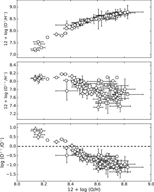
The O+ abundance (upper panel), the O++ abundance (middle panel) and the relative ionic abundance of the two species (bottom panel) are shown as a function of the total oxygen abundance.
4 TESTS ON THE METHOD
In this work we stacked spectra of several hundreds of galaxies per bin in order to enhance the S/N and detect the auroral lines needed for the application of the Te method. Of course, physical properties like electron temperatures and metallicities inferred from stacked spectra are meaningful only if they are a good representation of the average properties of objects that went into the stack. In particular, the risk is that few objects could dominate the contribution on auroral line fluxes, thus biasing the estimate of electron temperature, and consequently of metallicity, from stacked spectra. This work is also based on the assumption that galaxies with similar values for both [O ii] λ3727/Hβ and [O iii] λ5007/Hβ have similar metallicities.
In order to test our hypothesis and the stacking procedure, we took the sample of galaxies from Pilyugin et al. (2010a) with detected [O iii] λ4363 and [O ii] λλ7320, 7330, and stacked these spectra in bins of [O ii]/Hβ and [O iii]/Hβ according to our pipeline. For this analysis we considered only those bins with at least 15 objects, which namely are 0.4; 0.6, 0.4; 0.7, 0.5; 0.5 and 0.5; 0.6, as reported at the top of Fig. 8. Furthermore, we searched for those galaxies in our original sample (described in Section 2), with detection of [O iii] λ4363 in the MPA/JHU catalogue, falling into the same bins. In particular, we selected only galaxies with [O iii] λ4363 detected at ≥10σ.
![Histograms of Te method metallicities for the subsample of galaxies selected from Pilyugin et al. (2010a) with detected [O iii] λ4363 and [O ii] λλ7320, 7330 auroral lines (blue sample) and for galaxies with [O iii] λ4363 detected at >10σ from the MPA/JHU catalogue (red sample) for the 0.4; 0.6, 0.4; 0.7, 0.5; 0.5 and 0.5; 0.6 bin. The dashed lines indicate the metallicity inferred from the composite spectra obtained stacking the relative sample of galaxies. In every panel is also reported, for both subsamples, the difference between the average metallicity of the distribution and the value inferred from the associated stacked spectrum (Δ) and the number of objects per stack. The metallicity of the global stack, i.e. the stack obtained from the full sample of galaxies that fall in that bin, is written in the upper part of each panel and indicated by the dashed black line.](https://oup.silverchair-cdn.com/oup/backfile/Content_public/Journal/mnras/465/2/10.1093_mnras_stw2766/3/m_stw2766fig8.jpeg?Expires=1750229202&Signature=Ma15NAMtdqfmU~1~TJjLCUJ5fOc4SiMKocM-9qpvV0v~rU4qYFxYWUEB~jCE6wHr7ne8XRMtO969zqdGJyoVenF2qGwPvpSlUvtcACkJFXl9W7mnt5p~w-f1zEY5dSoNAzZwlZA4aGL8enet1VgnyvS3ACWw5Cr6XjNzCfF1DRhwA6QbHjAZQSNYiyQyCtqcLb8U~w4TY1HpkRaLajf~g~b-t0DgzDy1QMDT8Cms6C46fK0OL2U6JG~gcWrqJXRuIpv3ctLTBPHVEt6BHP~9TY1MJxQWo-Ylf2hy5aGkxFmxPNAK1EC7EUc3c25TR4kQ3fyEnd8KRV4iwz3yoJVOCg__&Key-Pair-Id=APKAIE5G5CRDK6RD3PGA)
Histograms of Te method metallicities for the subsample of galaxies selected from Pilyugin et al. (2010a) with detected [O iii] λ4363 and [O ii] λλ7320, 7330 auroral lines (blue sample) and for galaxies with [O iii] λ4363 detected at >10σ from the MPA/JHU catalogue (red sample) for the 0.4; 0.6, 0.4; 0.7, 0.5; 0.5 and 0.5; 0.6 bin. The dashed lines indicate the metallicity inferred from the composite spectra obtained stacking the relative sample of galaxies. In every panel is also reported, for both subsamples, the difference between the average metallicity of the distribution and the value inferred from the associated stacked spectrum (Δ) and the number of objects per stack. The metallicity of the global stack, i.e. the stack obtained from the full sample of galaxies that fall in that bin, is written in the upper part of each panel and indicated by the dashed black line.
Temperatures and metallicities were computed for each single galaxy in both samples. The sample of Pilyugin et al. (2010a) galaxies has both the oxygen auroral lines detected, thus we were able to directly infer the temperatures and abundances of both oxygen ionic species. Since only the [O iii] λ4363 auroral line is instead available for objects selected from the MPA/JHU catalogue, we used the ffO2 relation of equation (3) to determine the flux of the [O ii] λλ7320, 7330 auroral doublet and compute Te[O ii] and the O+ abundance. Then, we generated, for each bin, separate composite spectra for both samples and we measured Te and metallicities with the Te method from the stacked spectra.
Fig. 8 shows the histograms of metallicity distribution of individual galaxies in each bin for the Pilyugin et al. (2010a) sample (from now on: the blue sample) and the sample selected from the MPA/JHU catalogue (from now on: the red sample). We note the quite small range of metallicities spanned by single galaxies in each bin, with typical dispersions of 0.1 dex, consistently with the width of our binning grid. Even though we cannot perform the same test for higher metallicity stacks due to the lack of auroral line detection in single galaxies, this corroborates the assumption that galaxies belonging to a given bin of fixed [O iii] λ5007/Hβ and [O ii] λ3727/Hβ have similar metallicities and that we are thus stacking objects with similar properties in terms of oxygen abundance. The dashed lines in Fig. 8 indicate instead the metallicity inferred from the associated stacked spectrum for both samples. The difference between the average metallicity of single galaxies in a given bin and the one inferred from the stacked spectrum is reported as Δ; the number of objects per bin is also written. We note that abundances estimated from stacks are well matched to the average of the metallicity distributions in every bin, with offsets being at most 0.02 dex for both samples. However, both the red and blue samples could not be fully representative of the galaxy population inside each bin, which consist also of a large number of galaxies with no detection of auroral lines. Therefore, we compare the metallicity inferred from the stacked spectra of both subsamples with the one derived from the global composite spectrum, i.e. the spectrum obtained stacking all the galaxies included in that bin according to the procedure described in Section 2. These values are reported at the top of each box of Fig. 8 and indicated by the black dashed lines. We find good agreement between the global stack metallicity and the one inferred from the stacked spectra of the two different subsamples, with typical offsets on average of 0.04 dex, even though we note a systematic metallicity underestimation when considering the two subsamples with respect to the global one. This is probably due to the fact that, when creating the stacked spectra for the different subsamples, we are averaging upon the most metal-poor galaxies in the bin, which in fact have the auroral lines detected. This could bias the subsample stacks towards lower metallicities, but this effect is smaller both than our bin size and than the average uncertainty associated with abundance measurements in our stacks. We therefore conclude that different subsampling criteria inside the same bin do not dramatically affect the metallicity estimation from composite spectra and therefore that stacked spectra are effectively representative of the average properties, in terms of oxygen abundance, of the objects from which they are generated.
5 CALIBRATIONS OF STRONG-LINE METALLICITY INDICATORS
In order to extend the metallicity range covered by our calibrations, we add to our stacks a sample of single galaxies with robust detection of [O iii] λ4363. We selected galaxies from our original SDSS DR7 sample with [O iii] λ4363 detection at >10σ, and we recomputed the oxygen abundance for these galaxies according to the procedure described in the previous section. In particular, we derive Te[O iii] directly exploiting the [O iii] λ4363 value reported on the MPA/JHU catalogue and used the ffO2 relation of equation (3) to infer Te[O ii] and the O+ ionic abundance. Even though a part of these galaxies, although not all of them, is already included into our stacking grid, we are able in this way to directly account for some of the most metal poor galaxies of our sample, without averaging them into the stacking bins; thus, we can better constrain the low-metallicity region of our calibrations.
![Strong line diagnostics as a function of oxygen abundance for our full sample: small green stars represent the sample of single SDSS galaxies with [O iii] λ4363 detected at S/N >10, while circles are the stacks colour coded by the number of galaxies in each bin. Our best-fitting polynomial functions are shown as solid blue curves, while the dashed red line represents the Maiolino et al. (2008) semi-empirical calibrations. In the N2 and O3N2 diagrams also the Pettini & Pagel (2004) (dashed purple curve), Marino et al. (2013) (dashed green curve) and Brown et al. (2016) for Δ(SSFR) = 0 (dashed black curve) calibrations are shown. A publicly available routine to apply these calibrations can be found at http://www.arcetri.astro.it/metallicity/.](https://oup.silverchair-cdn.com/oup/backfile/Content_public/Journal/mnras/465/2/10.1093_mnras_stw2766/3/m_stw2766fig9.jpeg?Expires=1750229202&Signature=giXKCKMWTWkC-nm1y2k69hTgR6EiyN7IRDpB6FAcEhZBCWpajAbz9TIE~YVr4aZcQB6RF1GVwCbTYHq66CsZBKuPfPz0Eo-srAZvUE6hUv7WR-Wpk5k-JqYhCnpSb7slUqh76Vcy-ti7MN39o-rINLntHdbXeHP0C2jueptW-Nlq3jmqOwGdUOYG3LEfQfZTuJSfZY-juMhtWSgV5lPqxk15cee3q0mIxRp1TUFO2YPDXGhr8K6nputoVHZTigHlWLrWBJyBsKdL~WuhKsL5zgsrSFRdVFf47bmiOoFf9FeAJyx2Ni64liSAGFi0yL7Gnhp9UknNXrwFVID1GtkmYA__&Key-Pair-Id=APKAIE5G5CRDK6RD3PGA)
Strong line diagnostics as a function of oxygen abundance for our full sample: small green stars represent the sample of single SDSS galaxies with [O iii] λ4363 detected at S/N >10, while circles are the stacks colour coded by the number of galaxies in each bin. Our best-fitting polynomial functions are shown as solid blue curves, while the dashed red line represents the Maiolino et al. (2008) semi-empirical calibrations. In the N2 and O3N2 diagrams also the Pettini & Pagel (2004) (dashed purple curve), Marino et al. (2013) (dashed green curve) and Brown et al. (2016) for Δ(SSFR) = 0 (dashed black curve) calibrations are shown. A publicly available routine to apply these calibrations can be found at http://www.arcetri.astro.it/metallicity/.
Best-fitting coefficients and rms of the residuals for calibrations of metallicity diagnostics given by equation (5). The σ parameter is an estimate of the dispersion along the log(O/H) direction in the interval of applicability given in the Range column.
| Diagnostic | c0 | c1 | c2 | c3 | c4 | rms | σ | Range |
|---|---|---|---|---|---|---|---|---|
| R2 | 0.418 | −0.961 | −3.505 | −1.949 | 0.11 | 0.26 | 7.6 < 12+log(O/H) < 8.3 | |
| R3 | −0.277 | −3.549 | −3.593 | −0.981 | 0.09 | 0.07 | 8.3 < 12+log(O/H) < 8.85 | |
| O32 | −0.691 | −2.944 | −1.308 | 0.15 | 0.14 | 7.6 < 12+log(O/H) < 8.85 | ||
| R23 | 0.527 | −1.569 | −1.652 | −0.421 | 0.06 | 0.12 | 8.4 < 12+log(O/H) < 8.85 | |
| N2 | −0.489 | 1.513 | −2.554 | −5.293 | −2.867 | 0.16 | 0.10 | 7.6 < 12+log(O/H) < 8.85 |
| O3N2 | 0.281 | −4.765 | −2.268 | 0.21 | 0.09 | 7.6 < 12+log(O/H) < 8.85 |
We then applied each calibration to our total sample of single galaxies and stacks and computed the differences between Te method metallicity and metallicity predicted by the calibration, in order to give an estimate of the dispersion along the log(O/H) direction, which is reported as σ in Table 2. For double-branched diagnostics (i.e. R3, R2 and R23) this estimate is provided only considering the metallicity range where they show monotonic dependence on log(O/H), which is reported in the Range column of Table 2. This column represents indeed the range of applicability for a given diagnostics when used as a single metallicity indicator. We note that σ should not be directly interpreted as the uncertainty to associate with metallicity determination with our calibrations, since uncertainties in emission line ratios could introduce comparable errors.
Since our calibrations are built from a non-homogeneous combination of single galaxies and stacks, dispersion in our diagrams is due to different contributions. In the range covered by single SDSS galaxies, it is the consequence of the intrinsic spread in a given strong-line ratio at fixed metallicity and of the uncertainty on the auroral line fluxes measurement. For the high-metallicity region covered by our stacks, since we are averaging on a large number of objects, the scatter due to the intrinsic dispersion should be in principle reduced. However, we must consider the effects associated with the particular choice of our stacking grid. Every stack has, by definition, a defined value of [O ii]/Hβ and [O iii]/Hβ; therefore, in the R2 and R3 calibration diagrams the residual dispersion reflects the segregation in a given diagnostic when the other is fixed. This means that for any given value of one line ratio, different metallicities can be found varying the other one. This is particularly clear in the R2 calibration, where different sequences for different [O iii]/Hβ values appear at metallicities above 8.2. Therefore, this diagnostic shows a clear dependence on oxygen abundance only in the low-metallicity regime, revealing how most of SDSS galaxies are falling in the transition zone between the two branches of this indicator. Thus, for the majority of our stacks the metallicity dependence is driven by [O iii]/Hβ, and indeed for this diagnostic the segregation in sequences of [O ii]/Hβ is much less prominent.
For other indicators, the dispersion mainly reflects the scatter for a given diagnostic line ratio inside each [O ii]/Hβ–[O iii]/Hβ bin. For each diagnostic the distribution of the corresponding line ratio inside our bins is generally strongly peaked, even though we are affected by different dispersions when considering different positions on our stacking grid. This means that a given line ratio, as measured from the stacked spectra, can be respectively more or less representative of the distribution of galaxies inside a given bin for different positions on the diagram. However, for every diagnostic ratio here considered, the typical dispersion of its distribution inside a given bin is of the order of 0.1 dex (or less), thus being consistent with the choice of our bin size.
In Fig. 9 we compare our new calibrations with those from Maiolino et al. (2008). They obtained semi-empirical calibrations combining direct abundance determination for galaxies from the Nagao et al. (2006) sample with metallicity estimation from theoretical models by Kewley & Dopita (2002). The two calibrations agree well, as expected, for most of the indicators at low metallicities, the main discrepancies arising in the high-metallicity regime where Te method metallicities of our stacks result lower than those predicted by photoionization models. This introduces a clear deviation in the slope in all our calibrations, that change significantly their steepness after 12 + log(O/H) ∼ 8.2. In fact, we note that the highest metallicities inferred from our composite spectra are only slightly higher (∼0.1 dex) than the solar value.
For the O3N2 and N2 indicators we can compare our calibrations also with empirical ones from Pettini & Pagel (2004) and Marino et al. (2013), who used single H ii regions and not integrated galaxy spectra to calibrate these line ratios against metallicity. Our calibrations have comparable slopes to those of Marino et al. (2013), but they present a systematic offset towards higher metallicities. This is probably due to the fact that calibrations entirely based on H ii regions like Marino et al. (2013) are biased towards high excitation conditions and low metallicities. Our N2 calibration is in good agreement with Pettini & Pagel (2004) at low metallicities but diverge, in the direction of predicting higher abundances, in the middle region. At metallicities close to the solar value this diagnostic begin to saturate, as expected from the fact that nitrogen becomes the dominant coolant of the ISM: the two calibrations then become comparable again. The O3N2 calibration instead presents a different slope than the Pettini & Pagel (2004) since the slope of their calibration is determined by the use of photoionization models at high metallicities due to the lack in their sample of H ii regions with direct abundances in that region of the diagram. We note that our calibrations are better constrained to be used for integrated galaxy spectra, since single H ii regions upon which most of the empirical calibrations are based on do not properly and fully cover the parameter space where many galaxies lie.
In Fig. 9 we also compare our calibrations for the N2 and O3N2 indicators with those derived by Brown et al. (2016), who derived oxygen abundances with the Te method from stacked spectra in bins of stellar mass and Δ(SSFR), i.e. the deviation of the specific star formation rate from the star-forming main sequence (SFMS; Noeske et al. 2007). Since they include Δ(SSFR) as a second parameter in their calibrations, we decide to plot here (in black) only the curves representative of SFMS galaxies, i.e. those obtained assuming Δ(SSFR) = 0. In fact, our galaxy sample is distributed around their SFMS representation (see equation 6 of Brown et al. 2016), with a small median offset of 0.009 dex. Their calibrations show an offset of ∼0.1 dex towards higher metallicities for both indicators with respect to ours. We note that our calibrations are more consistent with Brown et al. (2016) calibrations when considering their curves for Δ(SSFR) =−0.75.
In order to test the self-consistency of our calibrations, we applied them individually to our original sample of SDSS galaxies. Diagnostics behaving monotonically (i.e. N2,O3N2 and O32) can be compared over the full metallicity range spanned by our sample, to which we can straightly apply the calibration, while for those double valued we restricted our analysis to the interval given in the Range column of Table 2. Given that our R2 calibration mostly cover the transition zone for such indicator in our SDSS galaxy sample (i.e. for 12 + log(O/H) > 8.2), we decide not to include it in this analysis. In each panel of Figs 10 and 11, we show the histograms of the differences in metallicity estimation between a given diagnostic and all the others. Every strong-line indicator is identified by a different colour, and in each panel the name of the reference indicator is written in the upper region. The Δlog(O/H) is then evaluated as the difference between the metallicity probed by the reference indicator and the metallicities estimated with the other four; in each panel the average offset of the Δlog(O/H) distribution and the associated σ is reported.
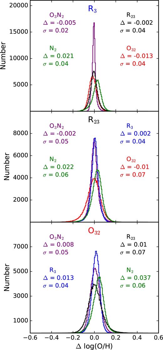
Upper panel: histograms of the difference between metallicities of the SDSS galaxies derived with the R3 calibration and through the other diagnostics. Each diagnostic is identified by a different colour: blue for R3, red for O32, black for R23, purple for O3N2 and green for N2. The average offset and σ of the Δ(O/H) distributions are written for every diagnostic with the associated colour. Middle panel: same as upper panel, with R23 as reference diagnostic. Bottom panel: same as upper panel, with O32 as reference diagnostic.

Inspection of the different panels of Figs 10 and 11 reveals that metallicities probed by different indicators are in good agreement among each other, with average offsets below 0.04 dex and typical dispersions below 0.1 dex. The little systematic metallicity overestimate reported for the O32 indicator and underestimate for the N2 indicator with respect to the others can be accounted for as a product of the fitting procedure. In this sense, the use of higher order polynomials allows to straighten the consistency of all our calibrations, since it minimizes the mutual disagreement between metallicities determined with different indicators. Thus, Figs 10 and 11 show that consistent metallicities are obtained in individual galaxies when using different calibrations, allowing to compare for example abundances obtained from diagnostics located in different spectral regions.
From the above considerations, we can say that our calibrations represent a self-consistent set totally based on the Te metallicity scale. This is important since at the present time there is not an established absolute abundance scale for galaxies. Most of the calibrations found in literature either rely on the assumptions of photoionization models or are based on individual H ii regions metallicities. In the first case the metallicity scale defined by models is inconsistent with the Te scale. In the second case, the emission line properties of H ii regions differ from those of integrated galaxy spectra and higher excitation conditions affect Te abundance estimation towards lower values. Until the number of high-metallicity galaxy with detected auroral lines will increase, allowing to build fully Te method calibrations based on samples of individual objects, our stacking technique represents a valuable approach to define Te-based calibrations. However, it should be stressed that metallicity estimates obtained from these calibrations are always affected by the particular choice of the stacking procedure. For example, the Brown et al. (2016) calibrations from stacked spectra in bins of stellar mass and Δ(SSFR) rely on a particular parametrization of the local star-forming main sequence and their metallicity predictions could differ from ours despite the fact that abundances are evaluated with the Te method in both cases.
In this work we chose to recalibrate the strong-line diagnostics relying only on the values assumed by galaxies on particular emission line ratios, thus assuming only the validity of the strong-line methods to infer metallicity from spectra of star-forming galaxies. In this way our calibrations could be in principle applied to a great variety of cases, in particular to large integral field unit (IFU) galaxy surveys that allow spatially resolved abundance studies [e.g. CALIFA, Sánchez et al. 2012; Mapping Nearby Galaxies at APO (MaNGA), Bundy et al. 2015 or Sydney-AAO Multi-Object Integral-Field Spectrograph (SAMI), Croom et al. 2012]. In such cases for example, the use of our calibrations allows to relax the assumption that scaling relations well assessed on global scales (e.g. the M–Z and the M–Z–SFR relations) still hold on smaller, local ones.
6 SUMMARY
We provided new and totally empirical calibrations for some of the most widely used strong-line diagnostics for the determination of oxygen abundance in star-forming galaxies. These relations have been derived combining a sample of single low-metallicity galaxies together with the stacking of more than 110 000 galaxies of the SDSS in bins of 0.1 dex in the log [O ii] λ3737/Hβ–log [O iii] λ5007/Hβ diagram, just assuming that galaxies with such similar strong-line ratios also show similar metallicity (i.e. assuming the validity of the so-called strong-line method). The increase in S/N provided by the stacking procedure allowed us to detect and measure both the [O iii] λ4363 and [O ii] λλ7320, 7330 auroral lines necessary to compute electron temperatures of the different ionization zones and apply the Te method for measuring metallicity on the full range of metal abundances spanned by galaxies in the SDSS survey. Here are summarized our main results.
We found evidence for [Fe ii] contamination of the [O iii] λ4363 auroral line in high-metallicity stacks (Fig. 3). This is one of the crucial lines for the application of the Te method for abundances estimation, thus we recommend care in using this line as electron temperature diagnostic when detected in high-metallicity (12 + log(O/H) ≳ 8.3) galaxy spectra.
We analysed the relations between electron temperatures of different ionization zones, finding that our stacks do not follow the established t2–t3 relation for H ii regions (Fig. 4). They show instead better agreement with a relation that correlates auroral and nebular line fluxes (ffO3 relation). Exploiting the direct detection of the [O ii] λλ7320, 7330 auroral doublet in all of our composite spectra, we provided a new relation (the ffO2 relation) for the determination of the flux of this auroral line (Fig. 6).
We then analysed the relations between some of the most common strong-line diagnostics and oxygen abundance in order to obtain a reliable calibration (Fig. 9). Our global sample allowed us to construct a set of calibrations, spanning more than 1 dex in metallicity, which are based on the uniform application of the Te method for oxygen abundance estimation on global galaxy spectra. All our calibrations are therefore defined, over their whole range, on a consistent absolute Te metallicity scale for local star-forming galaxies. The scatter around the best-fitting calibration varies between 0.05 and 0.15 for different indicators.
Comparing our new calibrations with different ones from literature reveals how our calibrations deviate significantly both from empirical ones based on H ii regions and from theoretical ones based on photoionization models, especially at high metallicities. In fact, we find that our most metal-rich stacks have oxygen abundance significantly lower than those predicted by models, and at most 0.14 dex higher than the solar one (i.e. ∼1.4 Z⊙). On the other hand, classical empirical calibrations obtained from H ii regions samples generally show lower metallicities for fixed line ratios, probably due to the fact that the single H ii regions used for those calibrations are somehow biased towards high excitation conditions in order to ensure auroral line detection at high metallicity.
We applied our calibrations to the original sample of SDSS galaxies. Metallicity estimates from different calibrations result in good agreement between each other, with typical average offsets lower than 0.04 dex and dispersions of the order of 0.05 dex. We do not find any systematic effect of metallicity overestimate or underestimate between the different diagnostics. Thus, our calibrations represent a self-consistent set that could be used in a variety of different cases depending on the availability of emission lines.
Acknowledgments
We gratefully acknowledge the referee for his/her constructive comments that improved this work.
MC acknowledges financial support from INAF for his PhD fellowship.
RM acknowledges support from the ERC Advanced Grant 695671 "QUENCH'' and support from the Science and Technology Facilities Council (STFC).
We greatly appreciate the MPA/JHU group for making their catalog public.
Funding for the SDSS and SDSS-II has been provided by the Alfred P. Sloan Foundation, the Participating Institutions, the National Science Foundation, the U.S. Department of Energy, the National Aeronautics and Space Administration, the Japanese Monbukagakusho, the Max Planck Society and the Higher Education Funding Council for England. The SDSS Web Site is http://www.sdss.org/.
The SDSS is managed by the Astrophysical Research Consortium for the Participating Institutions. The Participating Institutions are the American Museum of Natural History, Astrophysical Institute Potsdam, University of Basel, University of Cambridge, Case Western Reserve University, University of Chicago, Drexel University, Fermilab, the Institute for Advanced Study, the Japan Participation Group, Johns Hopkins University, the Joint Institute for Nuclear Astrophysics, the Kavli Institute for Particle Astrophysics and Cosmology, the Korean Scientist Group, the Chinese Academy of Sciences (LAMOST), Los Alamos National Laboratory, the Max-Planck-Institute for Astronomy (MPIA), the Max-Planck-Institute for Astrophysics (MPA), New Mexico State University, Ohio State University, University of Pittsburgh, University of Portsmouth, Princeton University, the United States Naval Observatory, and the University of Washington.
