


Abstract
We introduce a new method for estimating the covariance matrix for the galaxy correlation function in surveys of large-scale structure. Our method combines simple theoretical results with a realistic characterization of the survey to dramatically reduce noise in the covariance matrix. For example, with an investment of only ≈1000 CPU hours we can produce a model covariance matrix with noise levels that would otherwise require ∼35 000 mocks. Non-Gaussian contributions to the model are calibrated against mock catalogues, after which the model covariance is found to be in impressive agreement with the mock covariance matrix. Since calibration of this method requires fewer mocks than brute force approaches, we believe that it could dramatically reduce the number of mocks required to analyse future surveys.
1 INTRODUCTION
Covariance matrix estimation is a fundamental challenge in precision cosmology. In the standard approach many artificial or ‘mock’ catalogues are created that mimic the properties of the cosmological data set, the analysis is performed on each mock catalogue, and a sample covariance computed using those results. From a certain point of view this approach is very simple, since the mock catalogues are statistically independent of one another. The potential stumbling block is that the sample covariance provides a noisy estimate of the true covariance, and covariance matrix noise can degrade the final measurement. Reducing noise in the covariance matrix to acceptable levels generally requires a large number of mock catalogues, and covariance matrix estimation can consume the majority of computational resources for current analyses. Moreover, there is a clear trade-off between the number of mock catalogues required and the accuracy of any individual mock. We aim to improve this situation with a new method for covariance matrix estimation that combines simple theoretical results with a realistic characterization of the survey, and that can be calibrated against a relatively small number of mocks. We will demonstrate that this approach produces a covariance matrix suitable for analysis of baryon acoustic oscillations (BAO) in modern surveys.
The consequences of covariance matrix noise have been a subject of recent interest (Dodelson & Schneider 2013; Taylor, Joachimi & Kitching 2013; Percival et al. 2014). It is generally true that when cosmological parameters are determined from an observable estimated in Nbins (for example a correlation function or power spectrum), and the corresponding covariance matrix is estimated using Nmocks mock catalogues, then there is a fractional increase in the uncertainty in the cosmological parameters, relative to an ideal measurement, of |$\mathcal {O}\left(1/\left(N_{\mathrm{mocks}}-N_{\mathrm{bins}}\right)\right)$|. In other words, having Nmocks ∼ 10 × Nbins (rather than much larger) has an impact on the final parameter estimates comparable to reducing the volume of a survey by ∼10 per cent. When the covariance matrix is estimated using a sample covariance of mock catalogues, there is thus an incentive to make Nmocks − Nbins as large as possible.
While some current surveys have achieved Nmocks ∼ 100 × Nbins, we are concerned that this may not be achievable in future surveys. First, we expect that many future analyses will attempt to utilize more accurate mocks, for example incorporating realistic light cones, and that this will raise the computational cost of a single mock. In addition, many future surveys [e.g. Euclid (Laureijs et al. 2011), DESI (Levi et al. 2013), WFIRST-AFTA (Spergel et al. 2015)] have proposed to perform tomographic analyses, rather than analysing a single redshift range; where current analyses might estimate the correlation function using 40 bins, a tomographic analysis using 10 redshift slices will necessarily use 400 bins.
A number of approaches have been developed to mitigate this problem. Many authors have focused on decreasing the computational time required to generate a mock, thus enabling a larger number of mocks. For a discussion of this line of research, and a comparison of different methods, we refer the reader to Chuang et al. (2015). We emphasize that while available computing resources may increase at a pace that accommodates increasing mock requirements, there will always be an opportunity cost to producing large numbers of mocks – given fixed computing resources, reducing the number of mocks required by a factor of 100 means that the amount of computing time that can be spent on each mock increases by a factor of 100.
It is also possible to address the problem by reducing Nbins, rather than increasing Nmocks. For example, current BAO analyses typically compress the angular dependence of the correlation function into two multipole moments or a small number of angular wedges, rather than retaining the full angular dependence of the correlation function. Proposals have also been made for an analogous compression of redshift-dependence for tomographic analyses (Zhu, Padmanabhan & White 2015). While these approaches provide an intriguing complement to the method we will describe, we point out that there may be tension between the optimal modes for compressing the signal, and the characteristic modes associated with systematic effects. For example, reducing the angular dependence of the redshift space galaxy correlation function to monopole and quadrupole modes provides highly efficient compression of the underlying correlation function, but systematic effects tend to depend on line-of-sight or transverse separations between points and thus compress poorly into the monopole and quadrupole modes.
Rather than directly change Nmocks or Nbins, one can move beyond a simple sample covariance matrix. For recent efforts to develop phenomenological models of the power spectrum covariance matrix, see Pearson & Samushia (2016). Methods that take advantage of the sparsity of the precision matrix also present a promising avenue (Padmanabhan et al. 2016), as they provide low noise estimates of the covariance from a small number of mocks. For both of these approaches (and in the approach developed in this paper), it is important to understand if discrepancies between the approximated covariance matrix and the true covariance matrix will have an impact on the estimation of cosmological parameters.
The approach we will develop in this paper builds on a simple observation: that the covariance of a two-point function is an appropriately integrated four-point function. The foundational work on this approach is provided by Bernstein (1994), who provided explicit formulas for the covariance of the two-point correlation function of a non-Gaussian field observed in a finite volume with uniform number density. These integrals were recast in terms of the power spectrum by Cohn (2006), and Smith et al. and Sanchez et al. used these results to produce covariance matrices for a Gaussian field Poisson sampled in real space with uniform number density (Sanchez, Baugh & Angulo 2008; Smith, Scoccimarro & Sheth 2008). These efforts were primarily focused on producing covariance matrices suitable for use in forecasts, rather than analyses of existing data. They were later extended by Grieb et al. (2016) to redshift space, and to accommodate higher multipoles. Xu et al. (2012, 2013) used a similar model covariance matrix to analyse the clustering of luminous red galaxies in SDSS DR7. In order to bring the model into better agreement with mock catalogues, Xu et al. more carefully modelled the redshift space power spectrum and introduced modifications to the shot noise term, eventually fitting a four-parameter model to 160 mock catalogues. The resulting model covariance was found to be in good agreement with the mock covariance.
The approach we take in this paper is to work entirely in position space, using the correlation function instead of the power spectrum. We extend the results of Bernstein to accommodate a non-uniform number density and accompanying non-uniform weights, so that our model accurately reflects the geometry of a modern survey. We find that the necessary integrals can be performed with a relatively small investment of computational time – for the specific example considered in this paper, a noise level that otherwise would have required ∼35 000 mocks was achieved using only 1000 CPU hours. Rather than directly model the connected three- and four-point correlation functions, we find that their effects can be modelled by adjusting the level of shot noise in the model covariance matrix. We fit this single parameter using 1000 QPM mocks, although we find that a much smaller number of mocks would suffice to constrain the parameter. Extensive comparisons between our model covariance and the QPM mock covariance indicate that the model is suitable for use in cosmological analysis.
This paper is organized as follows. In Section 2 we provide a simple analytic expression for the covariance matrix of a galaxy correlation function. This extends the results of Bernstein (1994) to incorporate position-dependent number densities and weights. In Section 3 we numerically integrate this expression over a realistic survey geometry, assuming that the underlying galaxy field is Gaussian. We find reasonable agreement between our results and a sample covariance computed from 1000 quick particle mesh (QPM; White, Tinker & McBride 2014) mocks produced using the same survey geometry. In Section 4 we show that increasing the level of shot noise in the Gaussian model covariance matrix brings it closer to the full, non-Gaussian covariance matrix. After fitting the shot noise increase using the QPM mocks, we find exceptional agreement between our method and the QPM sample covariance. The methods developed here for comparing covariance matrices may be of interest to other researchers working on the covariance matrix problem.
2 N-Point Functions and the Covariance Matrix
In the following, we will demonstrate how to extend this simple result to correlation functions estimated in bins |$\Theta _{ij}^{a}$|; how to modify it for a Poisson-sampled density field, and how to incorporate the inhomogeneous number density and non-uniform weighting that occur in realistic surveys. We build on the foundational work of Bernstein (1994), who derived an integral expression for the covariance matrix of the correlation function of a non-Gaussian field estimated from a survey with finite volume and finite, uniform number density. Our introduction of inhomogeneous number density and non-uniform weighting are novel extensions of that work.
2.1 Poisson sampling
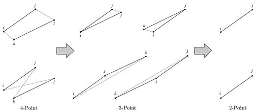
Configurations of points that contribute to the covariance matrix integrals. Starting from the two four-point configurations that contribute to C4, single contractions generate the four possible three-point configurations of C3, and double contractions generate the two-point configuration of C2. Solid lines indicate pairs of points that are governed by a binning function, |$\Theta ^{a}\left({\boldsymbol r}_{i}-{\boldsymbol r}_{j}\right)$|, while dotted lines indicate pairs of points that are governed by a factor of the correlation function, |$\xi \left({\boldsymbol r}_{i}-{\boldsymbol r}_{k}\right)$|.
3 INTEGRATING THE GAUSSIAN MODEL
In order to test the value of equations (23)–(26) for generating covariance matrices, we will attempt to reproduce the covariance matrix of a set of mock catalogues. Specifically, we will use 1000 QPM mocks (White et al. 2014) that mimic the CMASS sample of the Baryon Oscillation Spectroscopic Survey (BOSS). Redshift space distortions (RSD) are included, but no reconstruction algorithms have been applied to these mocks.
We use a correlation function estimated in 35 radial bins of width δr = 4 h−1 Mpc, covering r = 40–180 h−1 Mpc, and 10 angular bins of width δμ = 0.1, covering μ = 0–1. This is more bins, by at least a factor of 5, than would be used in a typical multipole analysis of BAO in the galaxy correlation function. A more aggressive binning was chosen in part because it makes the covariance matrix problem more challenging and makes the noise in the sample covariance matrix more readily apparent.
The numerical integration is performed with a new software package,1 ‘rascal: A Rapid Sampler for Large Covariance Matrices’. It allows flexible specification of the cosmology, redshift distribution, and model correlation function, and can accept angular completeness masks in the mangle format (Swanson et al. 2008). The sampling algorithm is described in Section 3.3.
3.1 Survey geometry
In order to compare our implementation of the survey geometry with that of the mock catalogues, we compare the values of RRa that we compute with the values taken from the mock random catalogues. The results are shown in Fig. 2. We find a small offset between our integration and the mocks which varies as a function of r⊥. This arises because the mocks are generated using a ‘veto mask’ which replicates holes in the survey smaller than the telescope field-of-view (e.g. areas obscured by bright stars). Querying this mask is quite time-consuming, and we have not used it when generating the samples in this paper.
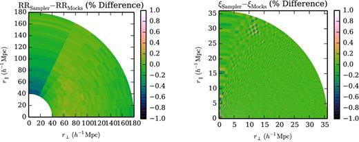
Using RR pair counts as a test of the survey geometry, we see that the representation of the survey in our sampler is in good agreement with the survey geometry in the mocks. We test the correlation function in our sampler by integrating it over the same bins used in the mocks, and find the two to be in excellent agreement.
3.2 Correlation function
In order to integrate equations (23)–(25) we must specify a model correlation function (not to be confused with the estimated correlation function, whose covariance matrix we are computing). Rather than use the linear theory correlation function, or one derived from perturbation theory, we use the non-linear correlation function estimated from the 1000 QPM mocks. This ensures that the correlation function we use for integration agrees at relatively short scales (r ≳ 1 h−1 Mpc) with the mocks, faithfully reproducing non-linear features such as the ‘finger-of-God’.
3.3 Importance Sampling
The integral (23) is 12-dimensional. It also has relatively limited support, so that the simplest Monte Carlo approaches converge quite slowly. We achieve acceptable convergence rates by using importance sampling. We begin by choosing a bin |$\Theta ^{a}\left({\boldsymbol r}_{i}-{\boldsymbol r}_{j}\right)$|, then generate uniform draws of the separation |${\boldsymbol r}_{i}-{\boldsymbol r}_{j}$| within that bin. We then draw |$\left|{\boldsymbol r}_{j}-{\boldsymbol r}_{k}\right|$| and |$\left|{\boldsymbol r}_{i}-{\boldsymbol r}_{\ell }\right|$| from a pdf proportional to r2|ξ0(r)|, where ξ0(r) is the spherically averaged correlation function. The angular components of |${\boldsymbol r}_{j}-{\boldsymbol r}_{k}$| and |${\boldsymbol r}_{i}-{\boldsymbol r}_{\ell }$| are again determined by uniform draws. Finally, we sort the sets of four points according to which bin |$\Theta ^{b}\left({\boldsymbol r}_{k}-{\boldsymbol r}_{\ell }\right)$| they fall in. We therefore are able to estimate one column of |$C_{4}^{ab}$| from a set of draws. Since the integration proceeds column-by-column, this approach is trivially parallelizable. Moreover, the same draws can be used to determine |$C_{3}^{ab}$| and |$C_{2}^{aa}$|.
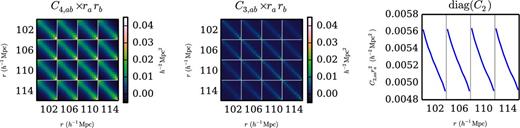
The three covariance matrix templates defined in (23)–(25), as evaluated using our sampler. The Gaussian covariance matrix is the sum of C4, C3, and the diagonal matrix C2. The correlation function is evaluated in bins with δr = 4 h−1 Mpc and δμ = 0.1. In these plots bins are ordered first in r (covering r = 102 h−1 Mpc to r = 114 h−1 Mpc), then in μ (μ = 0 to μ = 1). We show only a small portion of the covariance matrix, but this is sufficient to illustrate the high degree of convergence achieved in ∼1000 CPU hours with our sampler.
3.4 Comparison with mocks
We have constructed a simple Gaussian model for the covariance matrix, taking as inputs the survey geometry and non-linear correlation function. Given the modesty of these inputs and the simplicity of the Gaussian model, the close agreement between our model covariance matrix and the covariance matrix determined using 1000 QPM mock catalogues with the same geometry and correlation function is remarkable. In Fig. 4 we plot a portion of the precision matrix as determined from the mocks, as computed in the Gaussian model, and the difference between the two. We observe discrepancies between the two at the ∼10 per cent level, most noticeable for diagonal entries in the precision matrix and in entries for bins with the same μ that are adjacent in r, and we now investigate the consequences of these discrepancies.

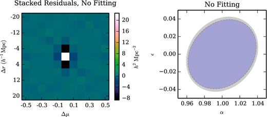
A small portion of the precision (inverse covariance) matrix, as determined from mock catalogues and from our Gaussian model (without fitting). The correlation function is evaluated in bins with δr = 4 h−1 Mpc and δμ = 0.1. In these plots bins are ordered first in r (covering r = 102 h−1 Mpc to r = 114 h−1 Mpc), then in μ (μ = 0 to μ = 1). The reduction in noise in the model precision matrix, relative to the mock precision matrix, is readily apparent. The residuals in the rightmost plot are surprisingly small, given that we are using the purely Gaussian model, but also indicate the need for non-Gaussian corrections to the model (see Fig. 6).
There are two reasons for using the precision matrix rather than the covariance matrix in this comparison. First, the structure of the precision matrix is considerably simpler than the structure of the covariance matrix, as can be seen by comparing Figs 3 and 4. Secondly, the precision matrix, rather than the covariance matrix, is what is used to compute χ2 statistics, and thus is the quantity that is most relevant in analysis. Finally, we point out that large eigenvalues of the precision matrix correspond to small eigenvalues of the covariance matrix, and vice versa, so agreement between precision matrices cannot easily be established by comparing the corresponding covariance matrices directly.
Comparison between the mock precision matrix and our (unfit) Gaussian model precision. Stacking the residuals reveals discrepancies on the diagonal of the precision matrix, and also for bins that share a μ range and are adjacent in r. Error ellipses for the BAO parameters α and ϵ show small discrepancies between the mocks (grey), model (blue), and noisy realizations of the model (dashed). The purely Gaussian model performs surprisingly well for BAO error estimation, but the discrepancies can be reduced with a non-Gaussian extension of the model (see Fig. 9).
It is telling that the discrepancies we observe between the mock and model precision matrices appear primarily on the diagonal of the precision matrix, and for bins that are adjacent to one another. Referring back to the integral in (23), we see that e.g. |$\left|{\boldsymbol r}_{i}-{\boldsymbol r}_{k}\right|$| and |$\left|{\boldsymbol r}_{j}-{\boldsymbol r}_{\ell }\right|$| can only reach very small values for overlapping or adjacent bins. We therefore interpret these discrepancies as a sign that our model is missing a contribution at short scales; since we know the two-point correlation function at short scales very well, it seems most likely that the observed discrepancies are a consequence of dropping the non-Gaussian terms involving ξ3 and ξ4. In the following we will attempt to model the non-Gaussian contributions without building explicit models for ξ3 and ξ4.
4 A SIMPLE MODEL FOR NON-GAUSSIANITY
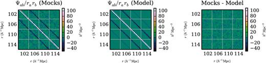
A small portion of the precision matrix, as determined from mock catalogues and from our non-Gaussian model (fit using the |$\mathcal {L}_{2}$| likelihood). The correlation function is evaluated in bins with δr = 4 h−1 Mpc and δμ = 0.1. In these plots bins are ordered first in r (covering r = 102 h−1 Mpc to r = 114 h−1 Mpc), then in μ (μ = 0 to μ = 1). The difference in the final plot shows that fitting has removed the residuals found in Fig. 4, so that the non-Gaussian model precision matrix is now in excellent agreement with the mock precision matrix.
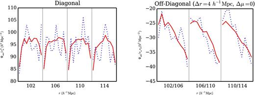
We plot here the most prominent parts of the precision matrices in Fig. 6, both from the mocks (blue, dotted) and from our non-Gaussian model (red, fit using the |$\mathcal {L}_{2}$| likelihood). The correlation function is evaluated in bins with δr = 4 h−1 Mpc and δμ = 0.1. In these plots bins are ordered first in r (covering r = 102 h−1 Mpc to r = 114 h−1 Mpc on), then in μ (μ = 0 to μ = 1).
In the following, we will develop two approaches for fitting CNG to the mocks. While the two approaches have distinct advantages and disadvantages, they will lead to substantially similar error ellipses for the BAO parameters α and ϵ.
4.1 |$\mathcal {L}_{1}$| likelihood
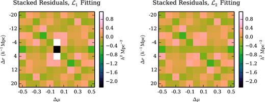
Stacked residuals between our non-Gaussian (fit) models and the mocks. Fitting the non-Gaussian model using the |$\mathcal {L}_{1}$| likelihood significantly reduces the stacked residuals relative to the (unfit) Gaussian model (see Fig. 5), while fitting with the |$\mathcal {L}_{2}$| likelihood effectively eliminates the residuals. The absence of residuals indicates that the model precision matrix could replace the mock precision matrix in a variety of applications.
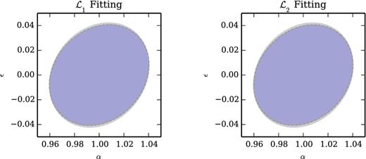
Error ellipses for the BAO parameters α and ϵ from the mocks (grey), the non-Gaussian (fit) models (blue), and noisy realizations of those models (dashed). The discrepancies between the mocks and the Gaussian (fit) model are reduced, though a 3 per cent discrepancy persists in σϵ. The similarity between the two error ellipses indicates that choice of likelihood (|$\mathcal {L}_{1}$| or |$\mathcal {L}_{2}$|) for fitting the non-Gaussian model has very little impact on BAO error estimation.
The principal benefit of the likelihood |$\mathcal {L}_{1}$| is that it does not require that we invert Cmocks. Indeed, this likelihood provides effective constraints on a (or other parameters, should we choose to fit a more elaborate model) even when Cmocks is degenerate, i.e. when Nmocks < Nbins. Although we will continue to use the full 1000 QPM mocks in our analysis, a much smaller number would have led to a very similar ΨNG. We anticipate that because this approach alleviates the need to have very large numbers of mock catalogues, it could be useful in a wide variety of cosmological analyses.
4.2 |$\mathcal {L}_{2}$| likelihood
The principal benefit of the |$\mathcal {L}_{2}$| likelihood is that it produces better agreement between the mock and model precision matrices than the |$\mathcal {L}_{1}$| likelihood, as shown in Fig. 8. Note that most (but not all) applications will require the precision matrix, rather than the covariance matrix. The principal drawback is that it requires that we invert Cmocks, and so requires that Nmocks > Nbins. In our case this requirement is satisfied, and so we prefer the |$\mathcal {L}_{2}$| likelihood. This preference is however slight, as the resulting α − ϵ error ellipses, shown in Fig. 9, are quite similar.
4.3 Results
One way to test the goodness-of-fit of our models is to determine what distribution of the KL divergence would result from noisy realizations of our best-fitting models. In order to ensure that the distributions we generate are comparable to the mocks, we do the following.
Draw 1000 correlation functions that follow our best-fitting covariance matrix.
Compute the sample covariance, Cnoisy, and corresponding precision matrix for those draws.
Fit Cnoisy or Ψnoisy as appropriate, to generate Crefit and Ψrefit.
Compute the KL divergence between the Cnoisy/Ψnoisy and Ψrefit/Crefit.
The results of these tests are collected in Table 1. We see that fitting with either likelihood provides a significant improvement over the purely Gaussian model. As anticipated, we find that fitting with the two likelihoods leads to small discrepancies in the resulting KL divergences. We also find that after fitting, the differences between the mock and model covariance matrices are too large to be consistent with noise, indicating that there is room for further improvement in our models.
KL divergences between our models (Gaussian, and Non-Gaussian fit using |$\mathcal {L}_{1}$| and |$\mathcal {L}_{2}$|) and the mock catalogues. In order to calibrate, we have also computed KL divergences between each model and fits to noisy realizations of that model. With 1000 mocks it is clear that the mock covariance matrix is not consistent with noisy realizations of our models.
| Ctest = Cmock | Ctest = Cnoisy | |
|---|---|---|
| KL(ΨG, Ctest) | 42.14 | 35.13 ± 0.17 |
| KL(ΨNG(a1), Ctest) | 37.66 | 35.13 ± 0.17 |
| KL(ΨNG(a2), Ctest) | 37.69 | 35.13 ± 0.17 |
| KL(Ψtest, CG) | 45.76 | 40.59 ± 0.27 |
| KL(Ψtest, CNG(a1)) | 42.70 | 40.59 ± 0.27 |
| KL(Ψtest, CNG(a2)) | 42.66 | 40.59 ± 0.27 |
In order to determine whether our model is sufficient to be used in studies of BAO, we return to the Fisher matrix approach introduced in Section 3.4. After computing the error ellipses, we would like to know whether the error ellipse from the mocks is consistent with a noisy draw from the model covariance matrix. To determine this we follow a procedure similar to the one described above: we generate sets of 1000 mock correlation functions drawn following the model covariance matrix, compute the sample covariance for those noisy draws, and then compute the error ellipse from that sample covariance. By repeating this procedure, we can arrive at uncertainties in the uncertainties in α and ϵ, σα and σϵ, as well as the uncertainty in their correlation coefficient, rαϵ. These results are tabulated in Table 2. We find that when focusing only on the α − ϵ error ellipses, and with only 1000 mocks, the models fit using |$\mathcal {L}_{1}$| and |$\mathcal {L}_{2}$| are indistinguishable, and are consistent at the 1σ level with the QPM mocks. This constitutes an improvement over the unfit Gaussian model, which is >2σ discrepant from the QPM mocks. Thus, while we would be reluctant to use the Gaussian model in some applications, the simple non-Gaussian model introduced here is suitable for use in contemporary BAO studies.
Fisher matrix results for the uncertainties σα and σϵ, as well as the correlation coefficient rαϵ. Even the Gaussian (unfit) model produces reasonable agreement in these parameters, and the level of agreement improves for the non-Gaussian (fit) models. When we restrict our attention to the BAO parameters, we find that the mock precision matrix is consistent with a noisy realization of our fit models, at least when we are limited to 1000 mocks.
| σα | σϵ | rαϵ | σα (noisy) | σϵ (noisy) | rαϵ (noisy) | |
|---|---|---|---|---|---|---|
| Cmock | – | – | – | 0.0403 | 0.0422 | 0.189 |
| CG | 0.0384 | 0.0391 | 0.216 | 0.0387 ± 0.0011 | 0.0394 ± 0.0011 | 0.217 ± 0.038 |
| CNG(a1) | 0.0400 | 0.0405 | 0.203 | 0.0403 ± 0.0011 | 0.0409 ± 0.0012 | 0.204 ± 0.038 |
| CNG(a2) | 0.0399 | 0.0404 | 0.204 | 0.0401 ± 0.0011 | 0.0407 ± 0.0011 | 0.205 ± 0.038 |
We have not addressed the question of precisely when this model can be used. It is possible that as the number density of a survey increases the actual structure of the three- and four-point functions will be detectable in the covariance matrix. This is an intriguing question, and one we anticipate addressing in future work. We emphasize that numerically evaluating the integrals 23 and 24 with the full 3- and 4-point functions would not require substantially more computational time, so that the general approach described in this paper would still be effective in a very dense surveys, even if the model described in this section were to break down. We also emphasize that in the QPM mocks2nPBAO ∼ 1, i.e. these mocks are not dominated by shot-noise. That our model is effective in this regime is very encouraging.
In the above we have used all 1000 QPM mocks to test our model precision matrix, since these are the most stringent tests we can perform with the mocks we have in hand. We can also imagine a scenario where we are interested in determining how many mock catalogues are required to appropriately calibrate our model precision matrix. A full treatment of this question requires that we specify accuracy goals for the precision matrix, and also raises the possibility that our model is better calibrated against something besides full-survey mocks (e.g. simulations of smaller sub-volumes of the survey, or against the survey data itself). We defer such a treatment for future work, focusing for now on the question of how the uncertainty in a depends on the number of mock catalogues used.
In Fig. 10 we show jackknife error bars for a computed using subsets of the full set of QPM mocks of size Nmocks. Because the fitting with the |$\mathcal {L}_1$| likelihood does not require that we invert the mock covariance matrix, we find the uncertainty in a is only weakly dependent on Nmocks. Indeed, we can achieve <1 per cent uncertainty in a with only 100 mocks, in spite of the fact that our covariance matrix has 350 bins. Fitting with the |$\mathcal {L}_2$| likelihood does require that we invert the mock precision matrix, and so we do require that Nmocks > 350, although we again achieve <1 per cent precision on a with only 600 mocks. As discussed above, fitting with the |$\mathcal {L}_2$| likelihood does provide a more accurate model precision matrix (Fig. 8), though this level of accuracy is not ultimately necessary for applications to BAO measurements (Table 2).
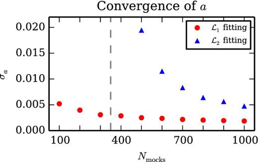
The uncertainty in the shot noise rescaling parameter a versus the number of mocks used to calibrate it. Our covariance matrix has 350 bins, and so we indicate with a vertical dashed line Nmocks = 350. As the |$\mathcal {L}_1$| likelihood (see equation 39) does not require that we invert the mock covariance matrix, it yields a precise estimate of a even with |$\mathcal {O}(100)$| mocks. The |$\mathcal {L}_2$| likelihood (see equation 43) does require that we invert the mock covariance matrix, and so only yields a precise estimate of a for Nmocks well above 350. Typical values for a in our model, calibrated against the QPM mocks, were 1.14, so 1 per cent precision on a can be achieved with a small number of mocks.
5 OUTLOOK
We have demonstrated that integrating a simple Gaussian model for the covariance matrix of the galaxy correlation function yields a result that is in surprising agreement with that obtained from sample statistics applied to mock catalogues. A simple extension of that model, wherein the shot noise is allowed to vary and calibrated against mock catalogues, further improves that agreement, so that for the purposes of BAO measurements the mock and model covariance matrices are statistically consistent with each other. This was accomplished with an effective number of mocks Neff ∼ 35 000 using just ≈1000 CPU hours, rather than the hundreds of thousands of CPU hours required to generate and analyse 1000 QPM mocks. Based on these results, we consider this method of covariance matrix estimation to be a strong alternative to producing very large numbers of mock catalogues. While |$\mathcal {O}\left(100\right)$| mocks will continue to be necessary for estimating systematic errors, we believe those |$\mathcal {O}\left(100\right)$| mocks will be sufficient to calibrate our model, or successors to it. With a reduction in the number of mocks required, we anticipate greater effort (both human and computational) can be devoted to improving the accuracy of the mocks, ultimately improving the reliability of error estimates from future analyses.
For the sake of simplicity we have focused on reproducing the mock covariance matrix. This is a somewhat artificial goal, since the mock catalogues are themselves imperfect representations of an actual survey. Turning our attention to the survey covariance matrix, we find an opportunity and a challenge. In our method, the mocks are only used to calibrate non-Gaussian corrections, in the form of increased shot noise, to the covariance matrix. Since we expect the effects of non-Gaussianity to be confined to relatively short scales, we can imagine performing this calibration step against simulations with a smaller volume and higher resolution, compared to the mocks. At the same time, we face the challenging question of how to bound possible discrepancies between our model covariance matrix and the true survey covariance matrix. While the accuracy requirements for a covariance matrix (whether derived from mocks or from a model) are ultimately determined by the science goals of a survey, the question of how to determine those requirements and assess whether they have been reached seems largely open.
A clear benefit of mock catalogues is that the same set of mocks can be used for measurement using a variety of observables (e.g. the power spectrum) and cosmological parameters (e.g. fσ8, often measured using RSDs). While we have constructed a model covariance matrix suitable for analysis of the galaxy correlation function at BAO scales, our goal of reducing the number of mocks required for future surveys cannot be realized until analogous methods are developed for the other analyses typical of modern surveys. The covariance matrix of the power spectrum has received theoretical attention from many authors (Takahashi et al. 2009, 2011; de Putter et al. 2012; Mohammed & Seljak 2014). Recent efforts (Carron et al. 2015; Grieb et al. 2016) have come close to presenting a usable model for the covariance matrix of the power spectrum, though the effects of a non-uniform window function have not yet been incorporated. We are optimistic that the necessary extensions of those models can be performed, reducing the required number of mocks for power spectrum analyses to be in line with the |$\mathcal {O}\left(100\right)$| necessary for correlation function analyses.
RCO is supported by a grant from the Templeton Foundation. DJE is supported by grant DE-SC0013718 from the U.S. Department of Energy. SH is supported by NASA NNH12ZDA001N- EUCLID and NSF AST1412966. NP is supported in part by DOE DE-SC0008080.
Funding for SDSS-III has been provided by the Alfred P. Sloan Foundation, the Participating Institutions, the National Science Foundation, and the U.S. Department of Energy Office of Science. The SDSS-III web site is http://www.sdss3.org/. SDSS-III is managed by the Astrophysical Research Consortium for the Participating Institutions of the SDSS-III Collaboration including the University of Arizona, the Brazilian Participation Group, Brookhaven National Laboratory, Carnegie Mellon University, University of Florida, the French Participation Group, the German Participation Group, Harvard University, the Instituto de Astrofisica de Canarias, the Michigan State/Notre Dame/JINA Participation Group, Johns Hopkins University, Lawrence Berkeley National Laboratory, Max Planck Institute for Astrophysics, Max Planck Institute for Extraterrestrial Physics, New Mexico State University, New York University, Ohio State University, Pennsylvania State University, University of Portsmouth, Princeton University, the Spanish Participation Group, University of Tokyo, University of Utah, Vanderbilt University, University of Virginia, University of Washington, and Yale University.
This research used resources of the National Energy Research Scientific Computing Center, a DOE Office of Science User Facility supported by the Office of Science of the U.S. Department of Energy under Contract No. DE-AC02-05CH11231.
An introduction to the package, as well as the python code, is available at: https://github.com/rcoconnell/Rascal.
We have not performed a careful study of the PATCHY mocks, which cover the same survey volume as the QPM mocks and were also created for the analysis of the BOSS survey. They differ in some quantitative aspects from the QPM mocks, and in particular more accurately reflect the bispectrum of the CMASS sample from BOSS (Kitaura et al. 2016). While it would be interesting to assess the impact of these quantitative discrepancies, in the absence of qualitative differences between the two sets of mocks we do not anticipate a qualitative difference in the performance of this model.
REFERENCES
