


Abstract
The double-averaging (DA) approximation is widely employed as the standard technique in studying the secular evolution of the hierarchical three-body system. We show that effects stemmed from the short-time-scale oscillations ignored by DA can accumulate over long time-scales and lead to significant errors in the long-term evolution of the Lidov–Kozai cycles. In particular, the conditions for having an orbital flip, where the inner orbit switches between prograde and retrograde with respect to the outer orbit and the associated extremely high eccentricities during the switch, can be modified significantly. The failure of DA can arise for a relatively strong perturber where the mass of the tertiary is considerable compared to the total mass of the inner binary. This issue can be relevant for astrophysical systems such as stellar triples, planets in stellar binaries, stellar-mass binaries orbiting massive black holes and moons of the planets perturbed by the Sun. We derive analytical equations for the short-term oscillations of the inner orbit to the leading order for all inclinations, eccentricities and mass ratios. Under the test particle approximation, we derive the ‘corrected double-averaging’ (CDA) equations by incorporating the effects of short-term oscillations into the DA. By comparing to N-body integrations, we show that the CDA equations successfully correct most of the errors of the long-term evolution under the DA approximation for a large range of initial conditions. We provide an implementation of CDA that can be directly added to codes employing DA equations.
1 INTRODUCTION
The long-standing three-body problem was initially motivated by studying planetary motions in the Solar system. The discoveries of extrasolar planet systems with rich orbital architectures have recently reinvigorated the research into this problem (see e.g. Holman, Touma & Tremaine 1997; Innanen et al. 1997; Mazeh, Krymolowski & Rosenfeld 1997). Unlike the nearly circular and coplanar planetary orbits in the Solar system, some exoplanets are found on eccentric and/or inclined orbits (see review by Winn & Fabrycky 2015 and references therein). In recent years, dynamical processes involving highly eccentric orbits have been invoked to interpret a wide array of astrophysical phenomena (see e.g. Mazeh & Shaham 1979; Kiseleva, Eggleton & Mikkola 1998; Blaes, Lee & Socrates 2002; Wu & Murray 2003; Perets & Fabrycky 2009; Perets & Naoz 2009; Thompson 2011; Antonini & Perets 2012; Katz & Dong 2012; Bode & Wegg 2014; Dong, Katz & Socrates 2014). Highly eccentric orbits can bring two of the bodies to close approaches near the pericentres that result in dissipative interactions, mergers or collisions. In particular, a popular class of mechanisms to explain the formation of observed short-period (order of ∼day) planetary and stellar orbits invokes tidal dissipation during close encounters in three-body systems (see e.g. Mazeh & Shaham 1979; Kiseleva et al. 1998; Ford, Kozinsky & Rasio 2000; Wu & Murray 2003; Fabrycky & Tremaine 2007; Katz, Dong & Malhotra 2011; Lithwick & Naoz 2011; Naoz et al. 2011; Socrates et al. 2012; Dong, Katz & Socrates 2013; Dawson, Murray-Clay & Johnson 2015). It has also been recently realized that the rate for mergers and collisions of white-dwarfs (WDs) can be significantly enhanced in field triple systems (Thompson 2011; Katz & Dong 2012) and quadrupole systems (Pejcha et al. 2013), and WD collisions in triples may be responsible for the majority of Type Ia supernovae (Katz & Dong 2012; Kushnir et al. 2013; Dong et al. 2015).
The orbital evolution of a particular three-body system for a given set of initial parameters can be accurately calculated using a computer with direct integration of the inverse-square law. While such calculations play a crucial role in studying the three-body problem, analytic approximations have turned out to be equally important by allowing a deeper understanding as well as providing efficient routes for calculating the evolution for a large ensemble of initial parameters. In fact, for many cases in relevant astrophysical settings, direct numerical integrations are prohibitive due to the large amount of initial conditions needed to be scanned and large numbers of orbits (thousands, millions or even billions) to compute.
Many powerful analytical tools have been developed over centuries to study the nearly circular and coplanar Solar system orbits, but many of them are not applicable for highly eccentric and inclined orbits. A pathbreaking analytical insight was achieved about half a century ago by Lidov (1962) and Kozai (1962), who solved the three-body problem analytically at all eccentricities and inclinations in the limit of high hierarchy – an inner binary, orbited by a distant third body (the perturber). They found that an initially nearly circular orbit of the inner binary can be excited to high eccentricity by an inclined perturber over long time-scales (i.e. secular time-scales). A large class of astrophysical-relevant systems are hierarchical for the simple reason that if they are not, one of the bodies can be ejected on a short time-scale. The Lidov–Kozai solution stands as a starting point for a wide range of studies involving high eccentricities and inclinations.
In the limit of high hierarchy, on short time-scales (time-scales comparable to the orbital periods), the time evolution of the system can be well described by two separate Keplerian orbits – (1) the (inner) orbit of the inner binary; (2) the outer orbit of the perturber orbiting the inner binary's centre of mass. Over long time-scales (longer than the outer orbital period), the two orbits exchange angular momentum periodically and their eccentricities and mutual inclinations oscillate, which are called the Lidov–Kozai cycles. The exchange of energy between the orbits is negligible over long time-scale, and thus their semimajor axis values a and aper are practically fixed in time. The evolution can be calculated analytically by expanding the interaction Hamiltonian to the leading (quadrupole) term in the small parameter a/aper and averaging the equations of motion over the orbits. Averaging over the inner orbit only is called ‘single-averaging’ (SA) and over both the inner and outer orbit is called ‘double-averaging’ (DA). Lidov (1962) and Kozai (1962) arrived at their solution by doing DA, and following their works, DA has since been widely used as the standard method to study and apply the Lidov–Kozai solution.
For moderately hierarchical systems (a/aper ≲ 100), it has been recently found that the unaccounted small errors in the approximation employed in the Lidov–Kozai solution may have significant effects on the orbital evolution. These fall into two broad categories – the long-term evolution of the system due to higher order terms in the expansion in a/aper and short-term evolution due to the non-secular effects:
(1) The small contribution of the next order term in the perturbation expansion of a/aper (the octupole term) may accumulate over many Lidov–Kozai cycles and result in significant changes in jz (Ford et al. 2000; Katz et al. 2011; Lithwick & Naoz 2011; Naoz et al. 2011). In some cases jz may cross zero so that the orientation of the inner orbit switches between prograde and retrograde with respect to the outer orbit (i.e. orbital flip). When jz crosses zero, extremely high eccentricities may be obtained.
(2a)Within one period of the outer orbit, jz experiences oscillations which are not described by the Lidov–Kozai approximation (Antonini & Perets 2012; Katz & Dong 2012; Bode & Wegg 2014). Very high eccentricities may be achieved if the amplitude of these oscillations is comparable to the magnitude of jz.
(2b) The change in angular momentum may be significant within one period of the inner orbit if the eccentricity is large (i.e. the angular momentum is already close to zero, and see Katz & Dong 2012; Antonini et al. 2016 for more discussions). This very short term change is crucial for head-on collisions as it allows the binary to avoid close passages or grazing encounters (thus avoiding tidal dissipation or tidal disruption or strong GR precession) in the orbits prior to the actual collision (Katz & Dong 2012).
In this paper, we show that the short-term oscillations ignored by the DA approximation can accumulate over time and introduce significant errors in the long-term evolution of moderately hierarchical systems. This occurs when the mass of the perturber is not negligible compared to the central star. Our finding implies that the DA approximation employed in many previous studies of moderately hierarchical systems is inadequate and their results may need re-examinations. The problem is particularly severe when studying the effect due to the octupole term because it is a long-term effect which is significant for moderate hierarchy.
The significant error due to breakdown of the DA approximation had historical importance in celestial mechanics. When the approximation is used to estimate the apogee precession period of the Moon due to the perturbation of the Sun (precession of the longitude of the periapsis ϖ), a value of 18.6 yr is obtained, which is about twice the observed value. This led Euler, Delambert and Clairaut to suggest that Newtonian gravity required modification. The problem was eventually solved by Clairaut who corrected the averaging procedure to account for the short-term oscillations (for a historical review, see Bodenmann 2010).
The solution to the lunar problem by Clairaut and its further elaboration made use of the low eccentricity and inclination in the Earth–Moon–Sun system and therefore cannot be applied to study systems with high inclinations and eccentricities. Corrections for perturbers on circular orbits in the context of irregular moons around giant planets were recently derived by Ćuk & Burns (2004). We derive the leading-order correction terms (the corrected double-averaging – CDA equations) that are applicable to any eccentricity of the inner and outer orbit and arbitrary mutual orbital inclination. For simplicity we focus on the test particle case. We show that the CDA equations reduce the long-term error introduced by DA significantly with little extra computing expense.
2 THE DOUBLE-AVERAGING APPROXIMATION BREAKS DOWN OVER LONG TIME-SCALES
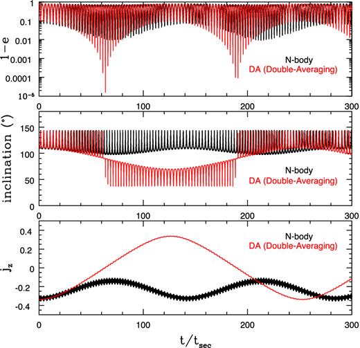
Significant difference in the long-term evolution of a three-body system using the exact N-body integration (black) and the approximated DA integration (red). The system consists of a test particle orbiting a mass m with semimajor axis a and a perturber with the same mass m. The outer orbit has semimajor axis aper = 10a and eccentricity eper = 0.2. The rest of the parameters are described in the text. The top, middle and bottom panels show the evolution of 1 − e, inclination and jz = (1 − e2)1/2cos i, respectively. The time is normalized to the secular time-scale tsec defined in equation (2).
This long-term breakdown of the DA approximation stems from ignoring the short-term oscillations in DA. This is demonstrated in Fig. 2. In the lower panel of Fig. 2, we show the results of the N-body and DA integrations, and they are also compared with the SA approximation where the equations are averaged only over the inner orbit. The potential in the SA approximation is expanded to the octupole term as for the DA equations, therefore the only difference between the SA and DA calculations is whether the outer orbit is averaged (in the DA case) or not (in the SA case). The results from SA is in good agreement with the N-body integration, implying that the main problem lies in the second averaging over the outer orbit.
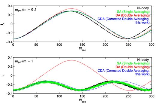
Lower panel: long-term evolution of the same system as the bottom panel in Fig. 1. Here besides N-body (black) and DA (red), we also include the results from integrating the SA equations (green) and the CDA equations (blue) derived in Section 3.2. Upper panel: long-term evolution of the same system as the lower panel except for a small perturber with the ratio between perturber mass and inner binary mass mper/m = 0.1. The failure of DA in capturing the long-term evolution stems from ignoring short-term oscillations on the period of the outer orbit. These short-term oscillations are taken into account by SA, which captures the long-term behaviour of the system. The long-term error of DA is larger for the stronger perturber, which induces short-term oscillations with higher amplitudes. See Fig. 3 for a closer inspection on the short-term oscillations.
The error in the second averaging is due to the small modulations in the orbital parameters of the inner orbit which occur within each outer orbit. These small oscillations can be clearly seen in the lower panel of Fig. 3, which shows the first Lidov–Kozai cycle of the same system as shown in the lower panel of Fig. 2. The upper panels of Figs 2 and 3 show the results of integration for a system with a less massive perturber mper = 0.1 m and all other initial conditions are identical with those shown in the lower panels. Clearly, the short-term oscillations and long-term errors are much smaller when the perturber is smaller. The effects of the short-term oscillations in Lidov–Kozai cycles were noted before (e.g. Antonini & Perets 2012; Katz & Dong 2012; Bode & Wegg 2014). Over a short time-scale, If the amplitudes of the short-term oscillations are large enough, they can bring jz to cross zero, which can lead to high eccentricities (see Section 1 and Katz & Dong 2012; Bode & Wegg 2014; Antonini et al. 2016).
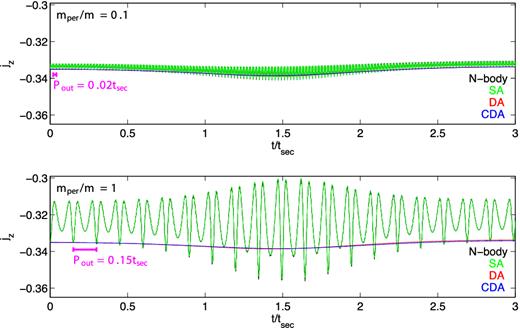
Zoomed views on the first Lidov–Kozai cycle of the same systems as shown in Fig. 2, allowing a close inspection on the short-term oscillations that are ignored by DA. The amplitudes for the short-term oscillations are lower for the less massive perturber shown in the upper panel.
Here we study the long-term effects of these short-term oscillations. In Section 3.2, we calculate these oscillations analytically and then we obtain the ‘corrected averaged double-averaged’ (CDA) equations by using these analytical results in the averaging over the outer orbit. The results of the integration of these equations are shown in Figs 2 and 3 as blue lines. As can be seen these equations are in good agreement with the SA approximation and the N-body integration. In Section 4 and Appendix Section A several more comparisons between N-body, DA and CDA integrations are performed.
3 CALCULATING THE SHORT-TERM OSCILLATIONS AND CORRECTING THE DA EQUATIONS
In this section, we derive analytical expressions for the short-term oscillations of |$\,\boldsymbol {j},\boldsymbol {e}$|. |$\boldsymbol {e}$| is a vector with magnitude e, and it points in the direction of the pericentre. We use these analytical results to derive corrections to the DA equations to account for their long-term effects.
Consider an inner binary of two objects with masses m2 ≤ m1 and a third body mper. We neglect the changes in the outer orbit which is assumed to be exactly Keplerian with parameters (aper, eper, Pout). This approximation is applicable when considering the short-term oscillations within one outer orbit discussed in Section 3.1 and also applicable to studying the long-term effects in two interesting physical cases: mper ∼ m1 ≫ m2 (the test particle limit) and mper ≫ m1 ∼ m2 (a binary system with comparable masses orbiting a much more massive object) for which the precession of outer orbit is negligible within the time-scale of interest1. As in Section 2, the z-axis is chosen to be in the direction of the angular momentum vector of the outer orbit and the x-axis pointing along outer orbit's eccentricity vector. We work with a moving coordinate system which is centred on the centre of mass of the inner binary, so the position vector of the two inner masses (m1 and m2), |${\boldsymbol r}_1$| and |${\boldsymbol r}_2$|, satisfy the relation |$m_1{\boldsymbol r}_1+m_2{\boldsymbol r}_2 = 0$|. The perturber's position |${\boldsymbol r}_{\rm per}(t)$| is confined to the xy plane and is parametrized by the radius |$r_{\rm per}= |{\boldsymbol r}_{\rm per}|$| and the true anomaly f (with f = 0 corresponding to y = 0, x > 0).
On short time-scales, the trajectory |${\boldsymbol r}(t)$| follows a Keplerian orbit which can be parametrized by the semimajor axis |$a= -0.5\ Gm(\dot{{\boldsymbol r}}^2/2-Gm/r)^{-1}$|, the normalized angular momentum vector |$\,\boldsymbol {j}= \mathbf {{\boldsymbol r}\times \dot{{\boldsymbol r}}}/\sqrt{Gma}$| and the Runge–Lenz vector |$\boldsymbol {e}= \dot{{\boldsymbol r}}\times ({\boldsymbol r}\times \dot{{\boldsymbol r}}/(Gm)-\hat{r})$| which points in the direction of the pericentre and has a magnitude |$|\boldsymbol {e}| = e$|. Due to the perturbation, these orbital parameters evolve with time.
3.1 Calulating the short-term oscillations analytically
DA ignores the small changes in |$\,\boldsymbol {j}$| and |$\boldsymbol {e}$| within the outer orbital period, and we show that such small changes can accumulate and cause a significant error for DA to characterize the long-term evolution of the system. Our task is to calculate such oscillations analytically and redo the averaging to include their effects to correct the DA equations. We will only consider the leading-order (the quadrupole term in equation 14) term of the small oscillations when calculating the oscillations. Note that in the sequent calculations, the corrections of the small oscillations to the leading order can be incorporated with the higher order terms (such as octupole) when doing the second averaging over the outer orbit.
The small parameter ϵSA defined in equation (20) sets the scale of the oscillations within one outer orbit. This is evident from equation (19) (noting that ϕ is dimensionless and of order unity). Another way to see this is that |$\,\boldsymbol {j},\boldsymbol {e}$| change by order unity over tsec and therefore change by order Pout/tsec during the time of one outer orbit Pout.
Equation (31) captures the short-term oscillations discussed in Section 2. To demonstrate this, the resulting oscillations in jz are compared to the results of the SA approximation in Fig. 4, which shows the same system as the bottom panel of Fig. 3. We first calculate |$\bar{\,\boldsymbol {j}},\bar{\boldsymbol {e}}$| by integrating the DA equations with the initial value of |$\bar{\,\boldsymbol {j}},\bar{\boldsymbol {e}}$| obtained from the initial value |$\boldsymbol {e},\,\boldsymbol {j}$|, f by solving (numerically) equation (34). The resulting evolution of |$\bar{j}_z$| is shown in dashed red. The only difference with respect to the DA approximation (shown in the figure in solid red) is the correction in the initial conditions which is henceforth denoted as initial phase correction (IPC). As can be seen in the figure, |$\bar{\,\boldsymbol {j}},\bar{\boldsymbol {e}}$| represent the middle of the oscillations between the two extremes. The oscillations are then calculated using equation (31) (or equivalently using equations 32 and 33) and shown in dotted magenta, which are in good agreement with the SA approximation (shown in solid green).
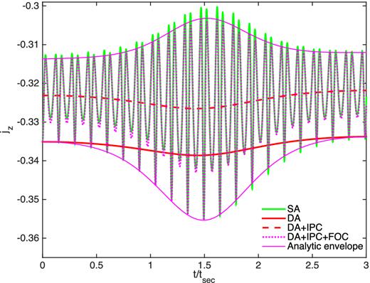
IPC and FOC. The results are for the same system as shown in the lower panel of Fig. 3. The results of a SA approximation calculation are shown in green, while the DA solution is shown in solid red. DA with IPC is shown in dashed red. For IPC, the initial conditions for |$\bar{\,\boldsymbol {j}}$| and |$\bar{\boldsymbol {e}}$| are found using the initial value of f and equation (31), and are later evolved using the DA approximation. We also show the FOC of jz using f and equation (32), shown in dotted magenta. The envelope of the oscillations is calculated using equation (35) and shown as solid magenta.
3.2 Correcting the double-averaging equations
We show the results by integrating the CDA equations in Fig. 5, and the three-body system is the same as shown in Fig. 1. As can be seen, the CDA equations manage to correct most of the long-term error present in the DA equations. In Sections 4 and A several more comparisons between N-body, DA and CDA integrations are performed.
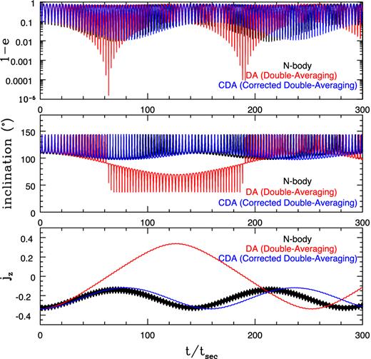
Comparison of the accurate N-body (black), DA (red) and CDA (blue) calculations for the same system and parameters as in Fig. 1. The results of the comparisons show that CDA captures the long-term characteristics in the evolutions of eccentricity, inclination and jz that are not captured by DA.
3.3 Implementation – using the equations in computer codes
A Matlab implementation of the equations presented in Sections 3.1 and 3.2 is provided in the supplementary text files. They are also provided at the following URLs for downloading:
http://arxiv.org/src/1601.04345v2/anc/CDA_Derivative.m
http://arxiv.org/src/1601.04345v2/anc/Integration_Example_System.m
http://arxiv.org/src/1601.04345v2/anc/Kepler_E_of_f_e.m
http://arxiv.org/src/1601.04345v2/anc/Quadrupole_Pout_Oscillation.m
http://arxiv.org/src/1601.04345v2/anc/Quadrupole_Pout_Oscillation_jz.m
http://arxiv.org/src/1601.04345v2/anc/Quadrupole_Pout_Oscillation_jz_maxmin.m.
The digital forms of the equations therein can be easily adapted to other programming languages. We provide below brief descriptions on what these codes do and how they can be used. The codes are also annotated with comments.
3.3.1 Long-term evolution using the CDA equations
The long-term evolution of the inner orbit can be calculated using equations (C1)–(C3). The CDA approximation equations are implemented in the file |$CDA\_Derivative.m$| which includes a function that calculates |${\rm d}\boldsymbol {e}/{\rm d}\tau$| and |${\rm d}\,\boldsymbol {j}/{\rm d}\tau$|. When setting ϵSA = 0, the function provides the (‘un-corrected’) DA approximation equations. We supply the parameters used in the example shown in Fig. 4 and the bottom panel of Fig. 3 in |$Integration\_Example\_System.m$|, and this script can be used to perform the integration to obtain the long-term evolution of the system shown in those figures. When integrating the DA or the CDA equations, a slightly better solution with the IPC can be obtained by converting the initial conditions of |$\,\boldsymbol {j},\boldsymbol {e}$| to the corresponding values of |$\bar{\,\boldsymbol {j}}, \bar{\boldsymbol {e}}$| using equation (31). IPC (see Fig. 4 and corresponding discussions in the text) can be done only if the initial value of the true anomaly f is specified. Parameters in the beginning of the file |$Integration\_Example\_System.m$| allow the users to choose to turn on or off IPC and whether to carry out calculations using the DA or CDA equations.
3.3.2 Short-term oscillations
The oscillations of |$\,\boldsymbol {j},\boldsymbol {e}$| within an outer orbital period can be calculated analytically using equations (31), (B1) and (B2) for given values of |$\bar{\,\boldsymbol {j}},\ \bar{\boldsymbol {e}}$|, eper, ϵSA (defined in equation 20) and f. This is implemented in the file |$Quadrupole\_Pout\_Oscillation.m$|. This result is applicable to first order to any configuration and set of masses (i.e. it is not limited to the test particle approximation). For calculating the oscillations of jz, equations (32)–(33) can be used, and they are implemented in |$Quadrupole\_Pout\_Oscillation\_jz.m$|. The envelope of the oscillations of jz is given by equation (35) and implemented in |$Quadrupole\_Pout\_Oscillation\_jz\_maxmin.m$|. The envelope is useful for long-term calculations in which it is desirable to avoid the relatively large number of time steps required to resolve the outer orbits. The short-term oscillations for the example system shown in Fig. 4 can be calculated with the script |$Integration\_Example\_System.m$| for the initial stages of the evolution. To do this, the values of |$\bar{\,\boldsymbol {j}}$|,|$\bar{\boldsymbol {e}}$| are calculated in the script by performing a long-term integration and are later used when calling the function |$Quadrupole\_Pout\_Oscillation\_jz.m$| to find the short-term oscillations.
4 COMPARISON OF N-BODY, DA AND CDA
In this section, we compare N-body, DA and CDA using large sets of initial conditions. We focus on comparing the conditions of orbital flips (i.e. whether jz crosses zero). The DA and CDA equations are integrated using the fourth-order Runge–Kutta method with a fixed time step dt = 0.05 tsec. Each run is stopped when reaching tmax = 10ϵOct−1tsec to make it sufficiently long for the octupole term to have a considerable effect. The N-body calculations are performed using the Wisdom–Holman splitting with adaptive time step described in Katz & Dong (2012). The presented examples are to illustrate some significant differences between DA and CDA for several large ensembles of systems. We stress that these examples are far from a complete survey of the parameter space, which is beyond the scope of this paper.
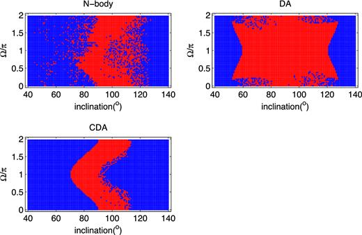
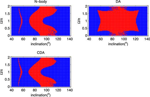
Fig. 6 shows the results of comparing N-body, DA and CDA integrations with changing orbital orientations. The integrations share the following parameters [mper/m = 1, aper/a = 10, eper = 0.2] and initially [ω = 0, e = 0.2]. The initial values of inclination and Ω are scanned. The choice of the initial true anomaly has insignificant effects here and is set to be 0 in the N-body calculations. For each simulation we record whether a flip occurs or not (i.e. whether jz crosses 0) during the entire run, and the results (flip/non-flip) are denoted as dots in different colours (red = flip, blue = no-flip). The IPC and Fast Oscillation Component (FOC) corrections (see Section 3.1) are not taken into account in the DA or CDA integrations. As can be seen from comparing with the N-body results (upper left), the DA integrations (upper right) fail significantly in capturing the bulk of the parameter space where orbital flips occur. CDA results (lower left) show good consistency with the N-body results. Similar comparisons for other sets of aper/a, e and eper are shown in Figs A1–A6.

Parameter space of orbital flips resulting from the N-body, DA and CDA integrations. Initial orbital parameters: mper/m = 1, ω = 0, eper = 0.2, aper/a = 10, e = 0.2. The initial values of inclination and Ω are scanned. For the N-body integrations, the true anomaly of both outer orbit and inner orbit are initially set to 0. Integrations in which flips occur (i.e. jz crossed zero) are shown as red points while those without are shown in blue. As can be seen, the DA calculations have significantly different results from N-body while CDA corrects most of the errors in DA.
In Fig. 7, the fraction of flips when scanning over Ω and fixing e = eper = 0.2 is shown as a function of inclination and the ratio of the semimajor axises. For each combination of the inclination and aper/a, 20 runs are performed with Ω uniformly distributed between 0 and 2π (step of 0.1π) to calculate the flip fraction. Different colours are used to denote different ranges of flip fractions with a step size of 0.25 (see caption). As can be seen, for the chosen masses and initial conditions, the flip fractions are similar between DA and CDA for aper/a ≳ 30 while there are substantial differences at smaller semimajor axis ratios.
![Orbital flip fraction as a function of inclinations and hierarchy (i.e. outer and inner semimajor axis ratios). The flip fraction is calculated for each combination of the inclination and semimajor axis ratio aper/a by performing 20 integrations with a range of Ω values between 0 and 2π in steps of 0.1π. All integrations have the initial parameters ω = 0, eper = 0.2, e = 0.2 and mper/m = 1. The results for integrations using the DA equations are shown in the left-hand panel and those using the CDA equations in the right-hand panel. The fraction (among the 20 runs) is illustrated by using different colour – blue = 0, magenta = (0,0.25], cyan = (0.25,0.5], green = (0.5,0.75], yellow = (0.75,1), red = 1.](https://oup.silverchair-cdn.com/oup/backfile/Content_public/Journal/mnras/458/3/10.1093_mnras_stw475/2/m_stw475fig7.jpeg?Expires=1749850443&Signature=DPq8rNhhxSu0IsVvW36LwfKjvQfaZbjeX~c5zHf8dsh4kiRCnJJZZ9EKC93NRxZ9h3HdWBluJyaCUv0RcfB4JBLgzY0~jRaPoG2xBlkD4VxGtCsgAiT9fz5i3TEJVMIpuLohz6pHzoMwuCzDFkD~FgKDmdsPjkcpc~cVXES02URKQjfa3WEUYD12fJuEYajdWOIdTUJBYnRmNMNodDp2wrPdQCfLEPOukc-iiejJSH4CVJITRI4G0NV22EiIYZ-7NSpgsztSgEYcdmuHs1L3o5aXCoX3nDp~j3A7LezHtNggBAjJb6dQjNZ4f9S8TF0aTczROX3quptUOMTqqMQgcA__&Key-Pair-Id=APKAIE5G5CRDK6RD3PGA)
Orbital flip fraction as a function of inclinations and hierarchy (i.e. outer and inner semimajor axis ratios). The flip fraction is calculated for each combination of the inclination and semimajor axis ratio aper/a by performing 20 integrations with a range of Ω values between 0 and 2π in steps of 0.1π. All integrations have the initial parameters ω = 0, eper = 0.2, e = 0.2 and mper/m = 1. The results for integrations using the DA equations are shown in the left-hand panel and those using the CDA equations in the right-hand panel. The fraction (among the 20 runs) is illustrated by using different colour – blue = 0, magenta = (0,0.25], cyan = (0.25,0.5], green = (0.5,0.75], yellow = (0.75,1), red = 1.
One generic feature that can be seen is a difference in the symmetry properties of the different approximations. In the DA approximation, the equations do not depend on the direction in which the perturber moves along the outer orbit (prograde or retrograde). The DA equations are therefore invariant under the transformation |$\,\boldsymbol {j}_{\rm per}\rightarrow -\,\boldsymbol {j}_{\rm per}$| which results in a change in our coordinate system |$(\hat{y}, \hat{z})\rightarrow (-\hat{y},-\hat{z})$| and therefore (inclination, Ω, ω) to (π − inclination, −π − Ω, ω + π). Combining this with the mirror symmetry with respect to the xy plane of the N-body equations z, vz − > − z, −vz, which results in (ez, jx, jy → −ez, −jx, −jy). This mirror symmetry does not affect the coordinate system or inclination but results in Ω, ω → Ω + π, ω + π. Combining the symmetries we obtain that the DA equations (to all orders in the expansion in ain/aout) are symmetric with respect to (inclination, Ω, ω) to (π − inclination, −Ω, ω). When sampling over all values of Ω, this implies a symmetry of the form inclination → π − inclination. As can be seen in Figs 6 and 7, while the results of the DA approximation respect this symmetry, the results of the N-body and CDA calculations violate this symmetry significantly. In particular note an interesting ‘island’ in the right-hand panel of Fig. 7 at inclination ∼50° and aper/a ∼ 10 where flips occur in the CDA calculations at relatively low inclinations with no counterparts on the retrograde region. No ‘islands’ exist in the DA results.
Finally, the flip fractions for isotropic distributions as a function of aper/a and mper/m are shown in Fig. 8. For each set we perform Monte Carlo simulations using the test particle DA and CDA equations for a wide range of values of aper/a and mper/m. For each combination of aper/a and mper/m, the flip probability is calculated using 1000 simulations with randomly chosen orientations drawn from an isotropic distribution (the cosine of inclination, Ω and ω follow uniform distributions). The initial eccentricities are fixed to e = eper = 0.2. The resulting flip probabilities as a function of aper/a for a number of perturber masses are shown in the left-hand panel of Fig. 8. As can be seen in the figure, the DA flip probabilities do not depend on the mass ratio mper/m while CDA probabilities do. In general the long-term correction is included in the CDA equations decreases the flip probability.
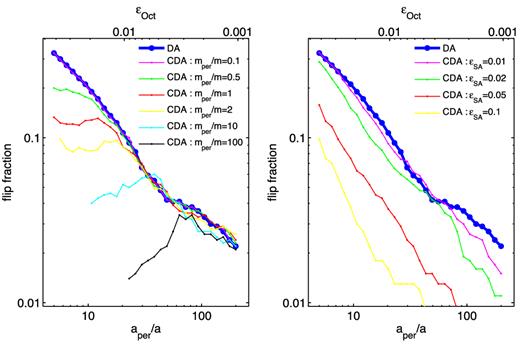
Flip probability for isotropic orientations as a function hierarchy (the outer and inner semimajor axis ratios) for different outer-to-inner mass ratios. The flip fraction is calculated for each combination of the mass ratio mper/m and semimajor axis ratio aper/a by performing 1000 integrations with orientations randomly chosen from an isotropic distribution. All integrations have the initial eccentricities eper = e = 0.2. Under the test particle approximation, the DA results are the same for all mass ratios (shown in blue) while the CDA results are presented for different mass ratios in different colours (see the legends and descriptions below). Left-hand panel: the flip probability as a function of aper/a for six fixed values of mper/m ranging from 0.1 to 100 shown in different colours (see the legend for the values and corresponding colours). Right-hand Panel: the flip probability as a function of aper/a for four fixed values of the expansion parameter ϵSA (equation 20) ranging from 0.01 to 0.1 shown in different colours (see the legend for the values and corresponding colours). For each combination of aper/a and ϵSA, the mass ratio mper/m is calculated using equation (20). As can be seen, significant differences between the DA and CDA calculations occur when ϵSA ≳ ϵOct, where ϵOct is the coefficient characterizing the strength of the octupole, shown in the top x-axis term (equation 17).
In the calculations presented so far in this section the effects of the ‘IPC’ and ‘FOC’ are usually small and have not been included. These effects become more significant when the perturber is more massive. To demonstrate this, the occurrence of flips as a function of orientation for a very massive tertiary, mper/m = 100 are shown in Fig. 9. As can be seen, for such massive perturbers, the IPC and FOC corrections are important.

Parameter space for orbital flips in the case of a massive perturber, mper/m = 100. The results of N-body, DA, CDA, CDA + ‘IPC’, and CDA+‘FOC’ (see Fig. 4 and related discussion in Section 3.1) are shown. Input orbital parameters: ω = 0, eper = 0.2, aper/a = 30, e = 0.2, f = 0 (for the N-body code the true anomaly of the inner orbit is also 0). As in Fig. 6, the results are shown as a function of the initial inclination and Ω and flip/non-flips are marked by red/blue points. As can be seen, for such massive perturbers the IPC and FOC corrections are required to capture the flips correctly.
5 DISCUSSION
Several previous authors have noted that the effects of short-term oscillations (on the outer orbital time-scale) on the Lidov–Kozai cycles are not captured by the DA approximation (e.g. Antonini & Perets 2012; Katz & Dong 2012; Bode & Wegg 2014). In this paper, we demonstrate that the short-term errors can accumulate over time, and the accumulated errors can significantly affect the long-term evolution of the system especially when the mass of the perturber is comparable or larger than that of the inner binary. In particular, the long-term evolution in the Lidov–Kozai cycles due to the octupole effect (Ford et al. 2000; Katz et al. 2011; Lithwick & Naoz 2011; Naoz et al. 2011) can be significantly affected by these errors, and as a result, the criteria for achieving orbital ‘flips’, where the mutual inclination between the inner and outer orbit crosses 90 deg leading to extreme eccentricities, can be considerably modified from the DA calculations (see Section 4).
The leading corrections to the secular equations due to the short-term oscillations in the test particle approximation are derived in Section 3. This is done by first deriving analytic expressions for the short-term oscillations (equations 31 and B1) and then incorporating them in the outer orbit averaging. The scale of the leading-order correction is set by the small parameter ϵSA defined in equation (20), which is roughly equal to the amplitudes of the variations of e, j within an outer orbit. The resulting CDA equations (equations C1–C3) are equivalent to adding the correction potential equation (39) to the standard doubly averaged potential equations (15)–(17). For the limiting case of eper = 0 and mper ≫ m, the potential reduces to that derived in Ćuk & Burns (2004, see however issue with ω mentioned below equation 39). The first-order corrections to the lunar precession are calculated in Section D and shown to agree with previous results. The equations are implemented in computer codes which are provided in the supplementary material and also on the web. They are described in Section 3.3. These can be used as standalone integration codes or added to existing secular codes.
As shown in Section 4 and Appendix Section A, the corrected equations capture most of the significant deviation between the N-body integrations and the DA integrations for a broad range of parameters. As can be seen in Fig. A1, at sufficiently low hierarchies, even the CDA equations fail to reproduce the N-body result. By examining a few of such runs, we find that even the single-averaged equations fail for this dynamically violent system with aper/a < 5, mper/m = 1, eper = 0.2 and ϵSA > 0.07. A systematic study on various kinds of errors of the DA equations not addressed by CDA as well as the regions in the parameter space where CDA is reliable, is beyond the scope of this paper.
We emphasize that, while the derived correction is in the test particle limit and thus its applicability is restricted to such systems, the long-term accumulation of the short-term errors found in this work occur under more general conditions. We are in the process of extending the derivations to relax the test particle approximation. Within the test particle approximation, these corrections can be added to other effects such as General Relativistic or tidal precession.
The long-term errors demonstrated in this paper may play an important role in a number of astrophysical settings in which the perturbers have considerable mass. Examples include triple star systems, planets in binary systems, binaries orbiting massive black holes and moons. Previous results studying such systems employing the DA approximation may need to be re-examined.
We thank Scott Tremaine and Dong Lai for helpful discussions. The work is partially carried out during LL's visit at the Weizmann Institute of Sciences (WIS), and we thank WIS for the supporting the visit. LL and SD are supported by ‘the Strategic Priority Research Program-The Emergence of Cosmological Structures’ of the Chinese Academy of Sciences (Grant No. XDB09000000) and Project 11573003 supported by NSFC. LL is partially supported by the Undergraduate Research Training program of Peking University. This research was partially supported by the I-CORE Program (1829/12). BK was partially supported by the Beracha Foundation.
Although the change in angular momentum of the outer orbit is small in these cases because it is always much larger than the angular momentum of inner orbit, the Runge–Lenz vector may change its direction within the time-scale of interest. The precession rate can be estimated as |${\rm d}\varpi _{{\rm out}}/{\rm d}\tau \sim L_{{\rm in}}/(L_{{\rm out}}\sqrt{1-e_{\rm per}^2})$|, where |$L_{{\rm in}} = \mu _{{\rm in}}\sqrt{Gma}$|, μin = m1m2/m and |$L_{{\rm out}} = \mu _{{\rm out}}\sqrt{G(m+m_{\rm per})a_{\rm per}}$|, μout = mmper/(m + mper). Our results are applicable for time-scales which are much smaller than (dϖout/dτ)−1tsec.
REFERENCES
SUPPORTING INFORMATION
Additional Supporting Information may be found in the online version of this article:
suppl_data
Please note: Oxford University Press is not responsible for the content or functionality of any supporting materials supplied by the authors. Any queries (other than missing material) should be directed to the corresponding author for the paper.
APPENDIX A: Extended parameter scan for flip citeria
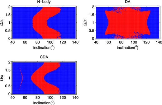
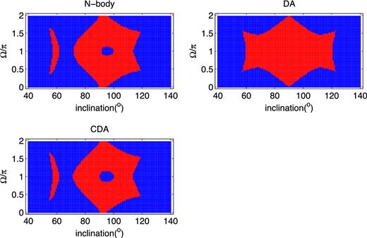
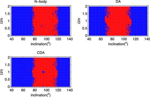
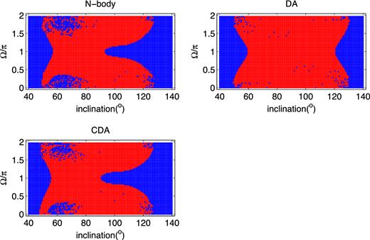
As an expansion of Section 4, the results of additional runs with different initial conditions are provided for N-body, DA and CDA calculations in Figs A1 –A6. In Figs A1–A4 the semimajor axis of the outer orbit is varied while all the other parameters are fixed. Fig. A5, is the same as Fig. A3, with aper/a = 8, but with the inner eccentricity starting at e = 0.01. Note the significant effect of the small eccentricity.
Same as Fig. 6 except initial aper/a = 5.
Same as Fig. 6 except initial aper/a = 6.5.
Same as Fig. 6 except initial aper/a = 8.
Same as Fig. 6 except initial aper/a = 16.
Same as Fig. 6 except initial e = 0.01 and aper/a = 8.
Same as Fig. 6 except initial eper = 0.8 and aper/a = 30.
Fig. A6 shows an example with a high value of the outer eccentricity eper = 0.8 (and correspondingly a larger aper = 30 to keep the outer orbit's pericentre away from the inner orbit). As can be seen this example, the CDA approximation is also quite reliable demonstrating the fact that the CDA equations are correct for high outer eccentricities.
APPENDIX B: Full analytical expression for Oscillating component
APPENDIX C: Full analytic expression for the Corrected doubly averaged equations
APPENDIX D: Application to the precession of the Moon's orbit
In this section the CDA approximation is applied to the precession of the Moon's orbit to verify that it reproduces the correct (known) precession rate to leading order.
In the Earth–Moon–Sun system, the orbit of the Moon is perturbed by the Sun. The Moon can be treated as a test particle. For the Earth–Moon–Sun system we have tsec = 2.1 yr, ϵSA = 0.075 and ϵOct = 4.1 × 10⁻⁵. The octuple and the |${\epsilon _{{\rm SA}}}e_{\rm per}^2$| correction terms are negligible.
If we use the doubly averaged equations, setting ϵSA = 0 we find that the periods of the nodal precession and apsidal precession have the same period of |$2\pi t_{\rm sec}/\frac{3}{4}\approx 17.7$| yr. The observed nodal precession period is 18.6 yr – 5 per cent accuracy; but the observed apsidal precession period is 8.9 yr – factor of 2 off. Leonhard Euler, Alexis Clairaut and Jean d'Alembert obtained the same puzzling result and were seriously considering the possibility that the 1/r2 gravitational law is wrong.
The first-order correction in ϵSA leads to a small correction to the nodal precession: 17.7 → 18.2 yr; but a large correction to the apsidal precession: 17.7 → 10.4 yr, bridging most of the gap to the actual precession rate (leaving 17 per cent error due to higher order terms). The reason that there is a significant correction even though the expansion parameter ϵSA is small, is due to the large pre-factor to the relative contribution of the first-order correction, |$\frac{225}{32}\frac{4}{3}\sim 10$|.
