


Abstract
The Baryon Acoustic Oscillation (BAO) feature in the power spectrum of galaxies provides a standard ruler to measure the accelerated expansion of the Universe. To extract all available information about dark energy, it is necessary to measure a standard ruler in the local, z < 0.2, universe where dark energy dominates most the energy density of the Universe. Though the volume available in the local universe is limited, it is just big enough to measure accurately the long 100 h−1 Mpc wave-mode of the BAO. Using cosmological N-body simulations and approximate methods based on Lagrangian perturbation theory, we construct a suite of a thousand light-cones to evaluate the precision at which one can measure the BAO standard ruler in the local universe. We find that using the most massive galaxies on the full sky (34 000 deg2), i.e. a K2MASS < 14 magnitude-limited sample, one can measure the BAO scale up to a precision of 4 per cent (∼1.2 per cent using reconstruction). We also find that such a survey would help to detect the dynamics of dark energy. Therefore, we propose a 3-year long observational project, named the Low Redshift survey at Calar Alto, to observe spectroscopically about 200 000 galaxies in the northern sky to contribute to the construction of aforementioned galaxy sample. The suite of light-cones is made available to the public.
1 INTRODUCTION
The combination of current and future dark-energy spectroscopic surveys will map the distance–redshift relation using the Baryon Acoustic Oscillation (BAO) as a standard ruler between redshift 0.2 and 2.5 down to 1–2 per cent within the next 5 years and 0.3 per cent within the next 10 years, this using multiple tracers: quiescent and star-forming galaxies, quasars and the Lyman α forest of quasars. These experiments will accurately determine the expansion history of the universe, and hence, will constrain its matter-energy content. As a complement to these probes, we should exhaust the information available in the local universe that is used to calibrate measurements at higher redshifts.
The total (systematics and statistics) uncertainty on the measurement of the Hubble constant today (H0), combining the supernovae data within a radius of <300 Mpc (redshift z < 0.08) whose distances are accurately determined with cepheids, is ±5 per cent (see Freedman & Madore 2010, for a review). This uncertainty should lower to ±2 per cent with the addition of James Webb Space Telescope (JWST).1
An alternative way to calibrate the distance–redshift relation would be to use the large-scale structure of the local universe, in particular the BAO feature in the clustering of nearby galaxies to measure both relations: the angular-diameter distance–redshift relation and the line-of-sight distance–redshift relation. The first estimates with the BAO standard ruler at low redshift were performed on the 6dF galaxy redshift survey, which samples 0.08 Gpc3 h−3 of the local universe with about 75 000 redshifts (Beutler et al. 2011). They measured the BAO scale at redshift 0.1 with a precision of 4.5 per cent and H0 with a precision of 4.8 per cent. Percival et al. (2010) obtained a 2.7 per cent precision on the BAO scale by analysing together the 2dFGRS and Sloan Digital Sky Survey (SDSS) data sets that contain 800 000 galaxies over 9100 deg2 at redshift z = 0.2 (corresponding to a volume of 0.2 Gpc3 h−3). Lately, Ross et al. (2015) reanalyzed SDSS-DR7 using only the most massive galaxies, and measured the BAO scale at redshift 0.15 with a 4 per cent precision. The precision on the BAO standard ruler in the local universe is today limited by the volume sampled by the surveys 6dF, 2dF and SDSS (Colless et al. 2001; Jones et al. 2009; Ahn et al. 2014). Now that the full-sky has been imaged by 2MASS and WISE (Skrutskie et al. 2006; Wright et al. 2010), there is a possibility of increasing the area (and thus the volume) observed by nearby galaxy spectroscopic surveys on to the full-sky limit. The BAO method, being subject to very low level of systematic errors (e.g. see Anderson et al. 2014 results for the BOSS survey), is a great way of making precise measurements of the local geometry of the Universe. Moreover a BAO measurement is orthogonal to the SNIa measurements in the standard parameter space of flat Λcold dark matter (ΛCDM) models. Thus, their combination will be very efficient in constraining the local distance–redshift relation, and hence the cosmological parameters (see Weinberg et al. 2013).
For the BAO probe in a limited volume, provided that a dense enough tracer allows overcoming the shot noise, the most suited tracer of the underlying dark matter density field is the one that maximizes the clustering amplitude (also called the bias). As the bias correlates with the stellar mass (Zehavi et al. 2011; Marulli et al. 2013), a sample that is closest to a mass-selected sample would meet this criterion. The most massive galaxies of the local universe are early-type galaxies and they have their bolometric luminosity dominated by the near-infrared light (1 to 5 μm) emitted by their evolved stellar population. This wavelength range is sampled by the 2MASS j, h, k bands (1.24, 1.66, 2.16 μm) and the WISEw1, w2 bands (3.35, 4.46 μm). All those bands correlate with the stellar mass and are suited to select massive galaxies in the low-redshift universe. The magnitude limit of the 2MASS surveys is shallower than that of WISE; k <14 compared to w1 < 17 (Vega magnitudes). But, the 2MASS k band being the most studied of all those bands for selecting galaxies, we choose the k band to construct our fiducial galaxy sample (see Section 2).
Then, we investigate the limits in precision of a full-sky BAO measurement at low redshift by analysing a series of mock catalogues of the local universe built using latest N-body BigMultiDark Planck simulations (Klypin et al. 2014) (see Section 3). Next, we use EZmocks (Chuang et al. 2015) to construct a reliable covariance matrix which will provide robust measurements of the uncertainties. We prove that the BAO measurement accuracy can reach 3.8 per cent with a full sky sample, 6.8 per cent with half of the sky and 12 per cent with a quarter of the sky (see Section 4).
In Section 4.7, we discuss the redshift error one can tolerate to obtain such a BAO measurement and show that current photometric redshift estimations are not precise enough. It is therefore timely to obtain spectroscopic redshifts of the full sky to extract all the cosmological information available.
To this aim, in Section 5, we propose a new galaxy spectroscopic redshift survey: the LoRCA survey.2 LoRCA will observe spectra for about 0.2 million galaxies of the north galactic cap that were not previously observed by SDSS with the best suited northern facility: the Schmidt telescope at the Calar Alto observatory. The LoRCA survey would be highly complementary to the Australian TAIPAN survey,3 which aims to observe of the order of a million low-redshift galaxies in the south galactic cap, starting in 2016.
Together, these surveys will enable the most detailed three-dimensional map yet of the local Universe and achieve the most precise measurement of the local BAO scale. Finally, in Section 6, we discuss additional cosmological probes with LoRCA: peculiar velocities, the galaxy mass function and strong lensing.
Throughout the paper, we assume Planck cosmological parameters |$\Omega _\Lambda =0.693$|, Ωm = 0.307 (Planck Collaboration XVI 2014).
2 GALAXY SAMPLE
The ideal galaxy sample that would maximize the clustering amplitude is a mass-selected sample. At z < 0.3, the magnitude that correlates best with the stellar mass is the k band (Kauffmann & Charlot 1998).
We therefore select a k < 14 magnitude-limited sample from the 2MASS full sky survey extended objects catalogue (Skrutskie et al. 2006). This catalogue contains all sources with a signal-to-noise ratio greater than 7 in at least one of the J, H, K bands, and some morphology criterion probing its extent.4 The extended source catalogue contains less than 1 per cent of artefacts and a very small population of stars, between 5 and 10 per cent depending on Milky Way stellar density. Target selection for LoRCA will be refined in a second phase using 2MASS point source catalogues and WISE ultimate photometric catalogues [see discussions in Kovács & Szapudi (2014) and Rahman et al. (2015)]. We keep extended objects with a galactic latitude |glat| > 10. Therefore, by masking the Milky Way from the extended source catalogue, we obtain a galaxy catalogue with purity >90 per cent. Note that for galaxies fainter than k > 14 the extended source catalogue is not complete. In total, we have 853 458 objects over 34 089 deg2 (82.6 per cent of the full-sky), i.e. a density of 25 galaxies deg−2. Note that by masking further the Milky Way |glat| >15 (20) the area diminishes to 30 575 deg2 (27 143).
To obtain a reliable expected redshift distribution of the selected target sample, we combine the following redshift catalogues: the third reference catalogue of bright galaxies (Corwin, Buta & de Vaucouleurs 1994), the SDSS DR10 (Ahn et al. 2014), the WiggleZ Survey DR1 (Drinkwater et al. 2010), the 6dFGRS DR3 (Jones et al. 2009), the GAMA DR2 (Taylor et al. 2011), the NASA-Sloan Atlas5 (Blanton et al. 2011) the 2MASS redshift survey (Huchra et al. 2012), and the 2dFGRS (Maddox 2000). In total, about 36.5 per cent of those targets already have a reliable spectroscopic redshift provided by one of those surveys mentioned above (see Fig. 1). A two sample Kolmogorov-Smirnov (KS) test shows that the available SDSS spectroscopic redshifts constitute a fair sample of the entire population (see left panel in Fig. 2). Hence, we infer the redshift distribution of the complete sample based on the current spectroscopic observations from SDSS. The right panel of Fig. 2 shows the galaxy counts as a function of k magnitude. We rescale the spectroscopic redshift distribution to obtain the same galaxy number density as in the 2MASS photometric selected sample (see Fig. 3).
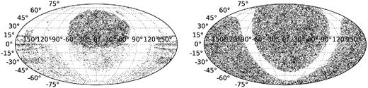
Dec. versus RA in degrees (J2000) of the 2MASS k < 14, |blat| > 10 galaxy sample that have been confirmed spectroscopically (left panel) and the map that LoRCA and TAIPAN will provide (right panel).

Left: k-band cumulative distribution function of the complete sample and the SDSS spectroscopic redshift sample. The KS test result shows that the spectroscopic sample is representative of the entire population. Right: Counts of all and galaxies with spectroscopic redshifts as a function of the K magnitude.
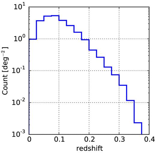
Extrapolated galaxy density (in deg−2) of the whole k < 14 2MASS target sample based on the already observed SDSS spectroscopic sample.
In Fig. 4, we compare the comoving density (in h3 Mpc−3) for the entire k < 14 galaxy sample, with the dark matter power spectrum. The linear component is computed using the Code for Anisotropies in the Microwave Background (CAMB; Lewis, Challino & Lasenby 2000) and the non-linear component is measured in the Multidark simulations. We assume a constant bias of 1.5 as found in Ross et al. (2015). The bias is slightly higher than the usual bias found for 2MASS galaxies due to the low-redshift cut applied, z > 0.07, to construct the clustering sample (Francis & Peacock 2010). The 2MASS k < 14 galaxy sample has n b2 P = 1 at r = 100 h−1 Mpc for z = 0.24. This galaxy sample is therefore useful to study the large-scale structure up to redshift ∼0.2; beyond that the density is too small to overcome shot noise. Note that the volume of the sphere with a radius z < 0.2 is 0.78 Gpc3 h−3 and that the volume covered by our sample footprint with |glat| > 10 is 0.64 Gpc3 h−3.
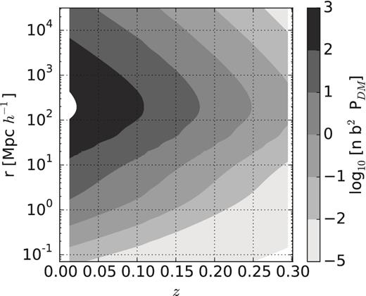
Scale versus redshift coded with log10n(z) b2 PDM(k, z), assuming a bias of b = 1.5. The contour labelled 0, corresponding to n(z) b2 PDM(k, z) = 1, is crossed for the scale 100 h−1 Mpc at redshift 0.24.
3 MULTIDARK MOCK CATALOGUES
The BigMultiDark Planck simulation (BigMD; Klypin et al. 2014,6) was run adopting a Planck ΛCDM cosmology (Planck Collaboration XVI 2014) using gadget-2 (Springel 2005) with 2.5 Gpc h−1 on the side and 38403 particles. Haloes were identified based on density peaks including substructures using the Bound Density Maximum (BDM) halo finder (Klypin & Holtzman 1997). We use BigMD to build the mock catalogues that will mimic the density of k < 14 galaxies drawn from the 2MASS survey and described above. Given the strong gradient in galaxy density as a function of redshift (see Fig. 3), we construct light-cones rather than use a single snapshot at the mean redshift of the sample (see below).
3.1 k-selected sample corresponding halo population
With our current BigMD mass resolution, it is not possible to mock the high galaxy number densities >0.007 h3 Mpc−3 observed at redshift z < 0.07 (the resolution is too low). We therefore construct a mock catalogue corresponding to a K-selected galaxy sample covering the redshift range 0.07 < z < 0.2. Observationally, the total density of k < 14 galaxies covering the redshift range 0.07 < z < 0.2 is 14.2 deg−2 or 0.0065 h3 Mpc−3. The volume lost by excluding z < 0.07 is 0.03 Gpc3 h−3 (i.e. 4.7 per cent of the total volume), leaving us with 0.61 Gpc3 h−3. Note that the line-of-sight comoving distance from redshift 0.07 is dC(z = 0.07) = 0.193 h−1 Gpc and from redshift 0.2 is dC(z = 0.2) = 0.572 h−1 Gpc.
We use 20 BigMD snapshots in the redshift range 0.07 < z < 0.2, and divide each simulation in eight subboxes of 1.25 Gpc h−1 on a side. In each of the eight subboxes we construct a light-cone using all 20 snapshots. We follow the standard procedure to construct light-cones from N-body simulations (Blaizot et al. 2005; Kitzbichler & White 2007).
Set the properties of the light-cone: angular mask, radial selection function (number density) and number of snapshots within the redshift range covered. We use each simulation snapshot within the redshift range to construct a slice of the light-cone; the redshift range of one slice from a snapshot at zi will be ((zi + zi − 1)/2, (zi + zi + 1)/2.
We position an observer (at redshift z = 0) at a point inside the box and we transform the coordinates of the box so that the observer is located at the Euclidean coordinates (x, y, z) = (0,0,0).
Sort all objects in each snapshot using the (sub)halo maximum circular velocity Vmax. This step is necessary because more massive objects (brighter galaxies) will have a larger priority in our selection when we apply a cut to fix the number density in the slice (radial selection function).
- Transform Cartesian coordinates to RA, DEC and rc (comoving distance in real space), which we use to compute the redshift of each object using the equation(1)\begin{equation} r_c(z)=\int \limits _0^z\frac{c {\rm d}z^{\prime }}{H_0\sqrt{\Omega _{\rm m}(1+z^{\prime })^3+\Omega _\Lambda }}. \end{equation}
Select in each simulation snapshot (sub)haloes such that (zi + zi − 1)/2 < z < (zi + zi + 1)/2 and |$\bar{n}(v>v_{\rm max})=\bar{n}(k<14,z)$| (Halo Abundance Matching, HAM). For that, we read the sorted objects until the expected number density is obtained. The angular selection function is a galactic longitude greater than 10: |glat| > 10.
Compute the peculiar velocity along the line-of-sight for each object to compute its distance in redshift-space |$\boldsymbol {s} =\boldsymbol {r}_c + (\boldsymbol {v}\cdot \hat{\boldsymbol {r}}) \hat{\boldsymbol {r}}/(aH)$|.
In this procedure, we assume that a k-selected sample is a stellar mass-selected sample and perform a HAM to reproduce the observed density of galaxies. This assumption is inaccurate in the sense that the true sample is not exactly complete in stellar mass. All the same, under this assumption, we derive the best possible BAO measurement in the local universe, i.e. we provide a lower limit to the precision one can reach with the most stellar mass complete spectroscopic survey of the local universe.
3.2 Comparison to data, small-scale clustering
Using the SDSS DR10 galaxy catalogue (Ahn et al. 2014), we can extract a galaxy sample that is representative of our k < 14 magnitude-limited sample by making the following cuts:
0.07 < z < 0.2 and ZWARNING≤4
k < 14 (2MASS magnitude)
130° < RA < 230° and 10° < Dec. < 55°
This sample contains 55 022 galaxies with a mean redshift at 0.12, and covers 7396 deg2 or a volume of 0.139 Gpc3 h−3 with a density of 7 per deg2. This average density is sufficient to overcome shot noise and measure the correlation function on scales smaller than 20 Mpch−1.
We draw randomly from the SDSS mask which removes the bright stars and the unphotometric areas. In Fig. 5 we compare the clustering measurement to the mean of the eight BigMultiDark mock light-cones. The agreement between data and simulation is very good in the range 0.8–10 h−1 Mpc.
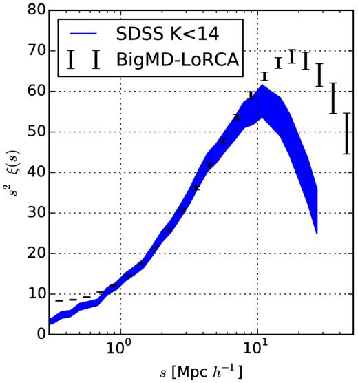
Two-point correlation function of the SDSS k < 14 galaxy sample compared to the mean and 1σ error bars of the BigMD mock light-cones.
We note two effects on smaller and larger scales. On smaller scales, we see the fibre collision effect, and hence no clustering enhancement on small scales below s < 0.8 h−1 Mpc. On larger scales, the clustering amplitude decreases at s > 20 h−1 Mpc due to the small volume of the sample, though the geometry allows for some large modes to be measured. Finally, this means the HAM models correctly reproduce the clustering of the galaxies we consider.
3.3 Massive mock production
We generate an additional 1000 mock light-cones using EZmocks (Chuang et al. 2015) to construct the covariance matrix for the measurement of the two-point correlation function. EZmocks have been designed to reproduce accurately, at very low computational cost, the large-scale structure of haloes in N-body simulations in terms of the two-point correlation function, power spectrum, three-point correlation function, and bispectrum, in both real and redshift-space (e.g. see Chuang et al. 2015). Thus, EZmocks is ideal for generating a large number of mock catalogues to construct a reliable covariance matrix for our local universe clustering measurements. To optimize computational resources, we derive the minimum number of snapshots necessary to make a truthful light-cone. We find that six redshift snapshots are sufficient to map the range 0.07 < z < 0.2. Hence, we produce 1000 realizations of the six snapshots to construct each EZmock light-cone of our local universe survey.
4 COSMOLOGY WITH THE BAO MEASUREMENTS FROM THE BIGMULTIDARK AND EZMOCK LIGHT-CONES
In this section, we describe the measurements of the correlation function obtained from the set of mock catalogues constructed using BigMD and EZmock. We also show the results of the likelihood analysis that leads to a constraint on the measurement of the BAO peak. Since we intend to provide an estimation of the expected constraint on the BAO measurement from our galaxy sample, we ignore some factors, which might introduce small bias to the mean value of the correlation function but should have negligible effect on the uncertainty.
4.1 Measuring the two-point correlation function
We use the two-point correlation function estimator given by Landy & Szalay (1993), with a bin size of 4 h−1 Mpc. This estimator has minimal variance for a Poisson process. The number of random points that we use is 10 times that of the number of data points. We assign to each data point a radial weight of 1/[1 + n(z) · Pw] (Feldman, Kaiser & Peacock 1994), where n(z) is the radial selection function and Pw = 2 × 10⁴h−3 Mpc3, as in Anderson et al. (2012). Fig. 6 shows each of the correlation functions from the individual eight BigMD mock catalogues, comparing with the mean correlation functions and 1-sigma error bar from the 1000 EZmocks described in Section 3.3.
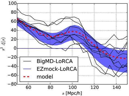
The two-point correlation functions from the eight BigMD-LoRCA mock catalogues (solid black lines) are compared with the 1σ region obtained from the 1000 EZmocks (blue region). The theoretical model is also shown (solid red).
4.2 Measuring the covariance matrix

Normalized covariance matrix based on the 1000 EZmocks coded after |$O_{ij}=\frac{C_{ij}}{\sqrt{C_{ii}C_{jj}}}$| where |$C_{ij}=\frac{1}{N-1}\sum ^N_{k=1}(\bar{\xi }_i-\xi _i^k)(\bar{\xi }_j-\xi _j^k)$|.
EZmock light-cone mocks have been calibrated with the simulation including the BAO signal. Therefore, they should be used for estimating the covariance matrix but not predicting the BAO significance. To obtain better forecast, one should use larger simulations or semi-N-body simulations (e.g. COLA; Tassev, Zaldarriaga & Eisenstein 2013) which are much more expensive than EZmocks; see Chuang et al. (2015)
4.3 Modelling the two-point correlation function
4.4 Likelihood analysis
We use CosmoMC (Lewis & Bridle 2002) in a Markov Chain Monte Carlo likelihood analysis. The only parameter we explore is α. We marginalize over the amplitude of the correlation function and fix Ωmh2, Ωbh2, and ns to the input Planck cosmological parameters of the BigMD simulation.
4.5 Results of BAO and broad-band shape measurements
Table 1 shows the individual α measurements and χ2 per degree of freedom (d.o.f.) obtained from each of the eight full-sky BigMD mock light-cones. We also measure α for the average of the eight mocks (0.985), and estimate the average of their errors (0.038 ± 0.017), and χ2/d.o.f. (0.99). One can see that the average χ2/d.o.f is very close to 1, which confirms that our covariance matrix is reasonable. The expected uncertainty on the BAO measurement for the proposed local universe sample is less than 4 per cent. See also in Table 1 the results for replacing the mock correlation function by the linear correlation function. Since there is no BAO damping in the linear correlation function, this constitutes an estimation of the expected precision on alpha provided a perfect BAO reconstruction (the best measurement one can reach). We obtain 1.2 per cent.
The mean and standard deviation of the α parameter for each of the eight individual full-sky BigMD light-cones. We also show the average of the means and the average of the standard deviations. The last line shows the fit obtained by replacing the mock correlation function with the linear correlation function.
| Full sky | α | σα | χ2/d.o.f |
|---|---|---|---|
| Mock 1 | 1.001 | 0.051 | 0.60 |
| Mock 2 | 1.013 | 0.035 | 0.90 |
| Mock 3 | 0.939 | 0.029 | 1.06 |
| Mock 4 | 0.979 | 0.043 | 0.93 |
| Mock 5 | 0.966 | 0.022 | 1.13 |
| Mock 6 | 1.059 | 0.063 | 0.80 |
| Mock 7 | 0.936 | 0.027 | 1.49 |
| Mock 8 | 0.986 | 0.032 | 1.01 |
| Average | 0.985 | 0.038 ± 0.016 | 0.99 |
| Linear CF | 1.001 | 0.012 |
Therefore, even with this small volume survey, we conclude that a full-sky survey of galaxies with k < 14 can reach a precision of 1.2–4 per cent on the BAO standard ruler measurement.
Now, we cut each of the mocks in two or four to estimate the expected determination of α when using only half-sky (6dF survey-like) or a quarter-sky (SDSS survey-like). The results are summarized in Tables 2 and 3. With half-sky (quarter-sky) survey, the results show that one can measure α at the 7 per cent precision level (12 per cent), which could be reduced by using a perfect reconstruction technique to 2.4 per cent level (5.3 per cent). Beutler et al. (2011) measured BAO (without using reconstruction) with 4.5 per cent precision using the 6dF survey, and Ross et al. (2015) measured BAO using the main SDSS survey at the 3.8 per cent precision level using reconstruction. Considering our analysis, both error estimates seem to be too optimistic.
Same as Table 1, but uses 6dF survey-like mock light-cones for half-sky.
| Half-sky | α | σα | χ2/d.o.f |
|---|---|---|---|
| 6dF mock 1 | 0.959 | 0.071 | 0.89 |
| 6dF mock 2 | 0.957 | 0.083 | 1.02 |
| 6dF mock 3 | 0.948 | 0.064 | 0.72 |
| 6dF mock 4 | 1.038 | 0.055 | 1.65 |
| 6dF mock 5 | 0.948 | 0.046 | 0.75 |
| 6dF mock 6 | 0.927 | 0.083 | 1.14 |
| 6dF mock 7 | 1.102 | 0.078 | 0.77 |
| 6dF mock 8 | 0.987 | 0.077 | 0.68 |
| 6dF mock 9 | 0.958 | 0.033 | 0.69 |
| 6dF mock 10 | 0.939 | 0.057 | 0.79 |
| 6dF mock 11 | 0.992 | 0.058 | 0.60 |
| 6dF mock 12 | 1.107 | 0.062 | 1.58 |
| 6dF mock 13 | 0.922 | 0.056 | 1.13 |
| 6dF mock 14 | 0.951 | 0.101 | 0.61 |
| 6dF mock 15 | 1.063 | 0.079 | 0.98 |
| 6dF mock 16 | 0.959 | 0.083 | 0.53 |
| Average | 0.985 | 0.068 ± 0.017 | 0.91 |
| Linear CF | 1.002 | 0.024 |
Same as Table 1, but uses SDSS survey-like mock light-cones for a quarter-sky.
| Quarter-sky | α | σα | χ2/d.o.f |
|---|---|---|---|
| SDSS mock 1 | 1.019 | 0.075 | 0.87 |
| SDSS mock 2 | 1.01 | 0.16 | 1.76 |
| SDSS mock 3 | 1.06 | 0.13 | 0.70 |
| SDSS mock 4 | 1.06 | 0.14 | 0.81 |
| SDSS mock 5 | 1.14 | 0.11 | 0.53 |
| SDSS mock 6 | 0.97 | 0.14 | 0.87 |
| SDSS mock 7 | 1.048 | 0.069 | 1.38 |
| SDSS mock 8 | 1.05 | 0.10 | 0.68 |
| SDSS mock 9 | 1.028 | 0.087 | 1.10 |
| SDSS mock 10 | 1.03 | 0.12 | 0.79 |
| SDSS mock 11 | 0.92 | 0.12 | 1.02 |
| SDSS mock 12 | 1.02 | 0.19 | 0.81 |
| SDSS mock 13 | 0.99 | 0.16 | 0.94 |
| SDSS mock 14 | 1.11 | 0.18 | 0.80 |
| SDSS mock 15 | 0.99 | 0.13 | 0.76 |
| SDSS mock 16 | 1.01 | 0.12 | 0.76 |
| SDSS mock 17 | 1.016 | 0.071 | 1.03 |
| SDSS mock 18 | 1.01 | 0.15 | 1.33 |
| SDSS mock 19 | 1.02 | 0.11 | 0.79 |
| SDSS mock 20 | 1.01 | 0.17 | 1.03 |
| SDSS mock 21 | 1.064 | 0.072 | 0.93 |
| SDSS mock 22 | 1.013 | 0.065 | 1.52 |
| SDSS mock 23 | 1.16 | 0.13 | 1.31 |
| SDSS mock 24 | 1.06 | 0.15 | 1.81 |
| SDSS mock 25 | 0.912 | 0.086 | 1.61 |
| SDSS mock 26 | 0.929 | 0.074 | 1.30 |
| SDSS mock 27 | 1.05 | 0.12 | 1.27 |
| SDSS mock 28 | 1.00 | 0.14 | 1.07 |
| SDSS mock 29 | 1.01 | 0.13 | 0.63 |
| SDSS mock 30 | 1.14 | 0.12 | 0.99 |
| SDSS mock 31 | 0.96 | 0.15 | 0.81 |
| SDSS mock 32 | 1.01 | 0.11 | 1.02 |
| Average | 1.026 | 0.12 ± 0.03 | 1.03 |
| Linear CF | 1.014 | 0.053 |
The mean and error on the α parameter for each of the eight individual full-sky BigMD light-cones including systematics.
| α(no systematics) | χ2/d.o.f. | α(with systematics priors) | χ2/d.o.f. | α (with double priors) | χ2/d.o.f. | |
|---|---|---|---|---|---|---|
| Mock 1 | 1.001 ± 0.051 | 0.60 | 0.997 ± 0.062 | 0.683 | 1.002 ± 0.075 | 0.685 |
| Mock 2 | 1.013 ± 0.035 | 0.90 | 1.011 ± 0.039 | 1.025 | 1.011 ± 0.042 | 1.017 |
| Mock 3 | 0.939 ± 0.029 | 1.06 | 0.932 ± 0.038 | 0.956 | 0.937 ± 0.050 | 0.819 |
| Mock 4 | 0.979 ± 0.043 | 0.93 | 0.967 ± 0.041 | 1.014 | 0.967 ± 0.053 | 1.017 |
| Mock 5 | 0.966 ± 0.022 | 1.13 | 0.956 ± 0.022 | 0.980 | 0.953 ± 0.027 | 0.986 |
| Mock 6 | 1.059 ± 0.063 | 0.80 | 1.055 ± 0.063 | 0.747 | 1.049 ± 0.063 | 0.693 |
| Mock 7 | 0.936 ± 0.027 | 1.49 | 0.946 ± 0.026 | 1.537 | 0.944 ± 0.027 | 1.537 |
| Mock 8 | 0.986 ± 0.032 | 1.01 | 0.989 ± 0.044 | 1.108 | 0.993 ± 0.057 | 1.112 |
| Average | 0.985 ± 0.038 | 0.99 | 0.982 ± 0.041 | 1.01 | 0.982 ± 0.049 | 0.98 |
4.6 Broad-band and systematics effects
4.7 Impact of redshift errors
In the previous sections, we assumed a perfect measurement of the redshift. We investigate the impact of eventual redshift errors on the estimation of the two-point correlation function. To this aim, we degrade. for example, the mock number 1 into observed mocks as follows.
We simulate redshift errors by drawing observed redshifts from a Gaussian distribution centred on the exact redshift with a scatter dz, i.e. |$z_{\rm obs}=\mathcal {N}(z_{\rm true},dz)$| with different values of dz: 0.0001, 0.0005, 0.001, 0.005, 0.01. For each value of dz, we produce 50 observed mocks on which we measure the correlation function. We take the mean of the 50 correlation functions as that obtained including redshift errors. In the scale range from 40 to 110 h−1 Mpc, the deviations from the original correlation function are smaller than 0.5 per cent for dz = 0.00005, 1 per cent for dz = 0.0001, 2 per cent for dz = 0.0005, 4 per cent for dz = 0.001, 25 per cent for dz = 0.005, and within a factor of 3 for dz = 0.01. Hence, we conclude that for dz≥0.005, the discrepancy between the observed and the true correlation function is larger than the statistical error predicted by the mocks. A reasonable aim for the spectroscopic redshift precision of a local universe BAO survey is dz ≤ 0.001, which can be achieved by a R ≥ 1000 spectrograph.
We simulate catastrophic redshift errors by shuffling a certain percentage of redshifts: 0.5, 1, and 5 per cent. On large scales, catastrophic redshifts have an impact below the percentage level if the fraction is below 1 per cent. On small scales, the clustering is underestimated by about 2 per cent for 1 per cent fraction of catastrophic redshifts. The main effect is that such errors damp the clustering signal at all scales. The fluctuations of the correlation function measurement due to such catastrophic redshift errors remain within the statistical errors.
We simulate systematic redshift errors by adding a fixed offset to all the redshifts, i.e. zobs = ztrue + offset, which takes the values 0.00005, 0.0001, 0.0005, and 0.001. This systematic redshift error strongly affects the measurement of the two-point correlation function. Even the smallest systematic error has a two per cent impact on large scales. The fluctuations of the correlation function estimation due to such systematic redshift errors remain within the statistical errors. Similarly to the catastrophic redshift errors, such uncertainty damps the signal at all scales.
In summary, the redshift errors described above would lead to a worse estimation of the two-point correlation function, and may introduce a damping of the BAO peak, but they do not shift the BAO scale.
The 2MASS full sky photometric redshift catalogue (Bilicki et al. 2014) currently has redshift errors of 0.015 which is much larger than the 0.005 required. It is therefore timely to obtain spectroscopic redshifts of the full sky to extract all the cosmological information (only 32 per cent were observed to date).
4.8 Probing dark energy
Probing cosmology is one of the key science drivers of most existing and upcoming redshift surveys, especially for the LoRCA + TAIPAN survey (LTs). We project the forecast on a Hubble diagram in the context of the ΛCDM paradigm (see Fig. 8). The improvement compared to previous BAO, SNe, is clear.

Aubourg et al. (2015) combined CMB, BAO and SNe, leaving curvature as a free parameter, and reported for a constant equation of state (EoS) for DE w = −0.98 ± 0.06. Allowing for a redshift varying EoS, although the significance is not yet strong enough to be conclusive, it shows a hint of dynamical dark energy (DDE) (Zhao et al. 2012). In this section, we perform a forecast for the sensitivity of LTs to probe the dark energy, in comparison with that of the SDSS-III BOSS survey (Alam et al. 2015).
4.8.1 Confirming the Fisher formalism
4.8.2 Constraints on DDE
Configuration I, the so-called CPL configuration (Linder 2003; Chevallier & Polarski 2001), is widely used in the literature for parameter constraints due to its transparent physical meaning [w0 = w(a = 1), w0 + wa = w(a = 0), wa = −dw/da] and simplicity. However, it cannot capture any dynamics of w(z) beyond the linear order of a. Configuration II is more general as w is essentially a freeform function. In this work, we use 40 bins, uniform in the scale factor from a = 1.0 to a = 0.5, and assume that w is a piecewise constant within each bin. The advantage of this configuration is that it allows model-independent study of w(z), such as the principal component analysis (PCA), which has been applied to dark energy studies (Huterer & Starkman 2003; Crittenden, Pogosian & Zhao 2009; Crittenden et al. 2012).
The result for the CPL configuration is shown in Fig. 9. As seen, adding in LTs improves the constraints on w0 and wa by 15 per cent and 14 per cent, respectively. Note that although LTs have no high-z ability, it can still improve the constraint on wa by breaking the parameter degeneracy. According to the Figure of Merit (FoM), as defined by the Dark Energy Task Force (DETF; Albrecht et al. 2006), the improvement is 17 per cent.
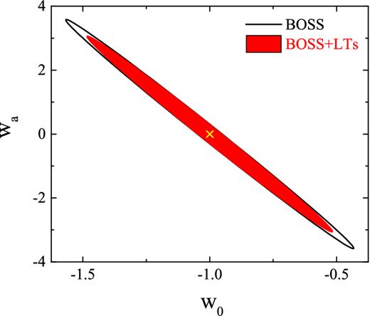
The 68 per cent CL contour plot for w0, wa using BOSS BAO data (black) and LTs (red filled), respectively. The cross denotes the fiducial model, which is the ΛCDM model.
The PCA result is shown in Figs 10 and 11. Fig. 10 shows the first three best constrained eigenmodes using BOSS and BOSS+LTs, respectively. BOSS alone does not have any sensitivity against the variation of w(z) at low redshift. However, when LTs are combined, the low-z sensitivity (at z < 0.2) is gained starting from the second eigenmode. The constraints on these modes are shown in Fig. 11. As shown, LTs improve the constraint on the second mode due to its low-z reach.
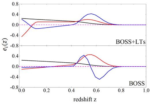
The first three best constrained eigenvector, defined in equation (11), using different combination of the data BOSS+LTs survey (upper panel) compared to BOSS alone (lower panel). The modes are shown, in the order from better constrained to worse as black, red and blue curves. The short dashed horizon line shows ei(z) = 0.
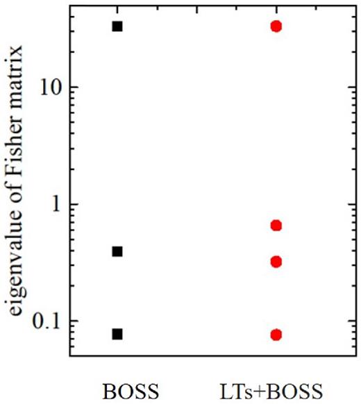
The eigenvalues of the BAO Fisher matrix for BOSS (black squares) and BOSS+LTs survey (red circles). Adding LTs to BOSS, one constrains one more mode.
In summary, covering the low-redshift ranges, LTs provide complementary dark energy constraints to BOSS. Assuming a CPL configuration of w(z), LTs improve the FoM by 17 per cent. A more general PCA approach reveals that LTs help detect the dynamics of dark energy at z < 0.2, which is crucial to dark energy studies (Linder 2006).
5 LORCA: THE LOW-REDSHIFT SURVEY AT CALAR ALTO
Considering this study, we propose the Low Redshift survey at Calar Alto (LoRCA) that aims observing ∼200 000 galaxies to complete the sample described above of ∼800 000 k < 14 galaxy redshifts in the northern sky.
Such a survey would constitute the northern counterpart of the first year of the Australian TAIPAN survey. Together, both surveys would reach the BAO precision limit reported in the previous section, and both LoRCA and TAIPAN will buildup the ultimate bright galaxy survey of the nearby universe. See the next section for other interesting science cases along with the BAO measurements.
This survey would use the Calar Alto 80-cm Schmidt telescope9 refurbished with a cartridge that hosts a plug aluminium plate that sits in the focal plane.
The field-of-view that we intend to cover with a single plate is 24 cm by 24 cm on the focal plane, i.e. 5| $_{.}^{\circ}$|5 × 5| $_{.}^{\circ}$|5. We plan to use 400 fibre robots to acquire the light from the targets. Fibre cables will measure about 15-m long. The fibre core will be 100 μm, which yield 8.6 arcsec on the telescope's focal plane.
We will use an existing spectrograph with sufficient (see below) resolving power R = 1100 that covers the wavelengths 3200 < λ < 7300 Å, which allows us to pack all 300 fibres on the pseudo-slit and map them on a 2k by 2k detector. Such resolution would allow estimation of the redshifts with an error better than dz ≤ 0.001.
Given that the SDSS data base (Ahn et al. 2014) already contains a fair spectroscopic sample of the galaxies to be observed, using a stacking procedure, we produced a library of high signal-to-noise ratio typical spectra of the LoRCA bright galaxy sample. We stacked the available SDSS spectra in three bins of redshifts and four bins of 2MASS K-band magnitude (see Fig. 12). In the first-redshift bin 0.07 < z < 0.1 (top panel), the 4000 Å Balmer-break is deep and the Hα emission line is well detected. In the highest redshift bin 0.15 < z < 0.2 (bottom panel), the Balmer-break feature is about two times weaker, though still very well defined, but the Hα line becomes weaker. The fainter 13.7 < k < 14 galaxies in the highest redshift bin should therefore drive the exposure time calculations. Note that the amount of features visible in absorption is sufficient to obtain reliable redshifts in ∼3.5 h exposures (signal-to-noise ratio above 10). Thus, it is not necessary to have a spectrograph that samples out to the Hα line. A sufficient wavelength coverage would be 3600 to 7200 Å, which is included in the currently available spectrograph (Hα goes out of the spectrograph at redshift 0.09).
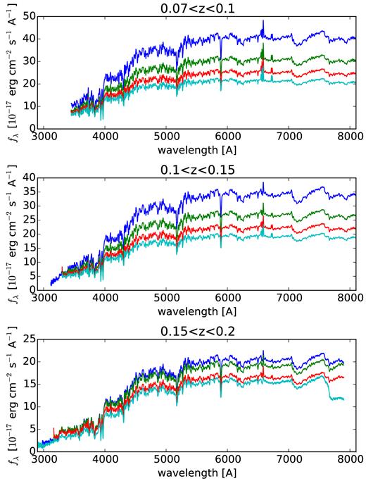
Typical SDSS spectra binned in redshift and K-band magnitude to be observed by the k < 14 LoRCA bright galaxy survey. In all panels, we show four mean stacked spectra corresponding to the magnitude bins: 12.5 < K < 13, 13 < K < 13.5, 13.5 < K < 13.7, 13.7 < K < 14 from bottom to top. Note the difference in the y-axis scale.
With the observational setting summarized in Table 5, we can plan the observation of two plates per night, including overhead of field acquisition and necessary calibrations. We aim to complete the observation of 200 000 redshifts with 700 plates in a 3-year survey that will cover half of the northern sky, starting 2016 (1 year after the start of TAIPAN), observing in dark time only and taking into account the average time lost due to bad weather at Calar Alto.
Summary of the parameters of LoRCA.
| Wavelength coverage | 3600 < λ < 7300 Å |
| Resolution | 1100 |
| Fibre aperture | 8.6 arcsec |
| Selection | k2MASS < 14 |
| N redshifts | 200 000 |
| N plates | 700 |
| Wavelength coverage | 3600 < λ < 7300 Å |
| Resolution | 1100 |
| Fibre aperture | 8.6 arcsec |
| Selection | k2MASS < 14 |
| N redshifts | 200 000 |
| N plates | 700 |
6 ADDITIONAL COSMOLOGICAL PROBES WITH LORCA
With the observational parameters specified for the BAO study, LoRCA can also address other key questions in cosmology.
6.1 Peculiar velocities
In the cosmology community there is a steadily increasing interest in measurements of peculiar velocities of galaxies. Koda et al. (2014) made a conclusive study discussing how new peculiar velocity surveys will be competitive as cosmological probes. Peculiar velocity can improve, for example, the growth rate constraints by a factor of 2 (and up to 5) compared to galaxy density alone.
The immediate use of peculiar velocities is for cosmic flows mapping in the Local Volume (Courtois et al. 2013). Large coherent flows allow one to study the structures formed by the total matter (dark and luminous) without the culprits of the redshift surveys which are probing only the bright galaxy distribution (Tully et al. 2014). Currently, this field is dominated in number by galaxy distances derived using H i radio-detections for the Tully–Fisher (TF) relation (Tully et al. 2013). However, the recent survey completed at the Schmidt telescope in Australia (Campbell et al. 2014) is now adding a similar number of Fundamental Plane galaxy distance estimates.
The second immediate use is for measurements of the local bulk flow and its physical interpretation for understanding the global motion towards the CMB dipole (Hoffman, Courtois & Tully 2015). When various scales are tested, comparisons are possible with the observed velocity field computed from the redshift surveys distribution of galaxies (Magoulas et al. 2013).
Finally, a third use for such surveys is to provide even better constraints on parameters of cosmological interest than a survey of redshifts alone (Burkey & Taylor 2004; Zaroubi & Branchini 2005). Comparing the galaxy–galaxy, galaxy–velocity and velocity–velocity power spectra (Johnson et al. 2014) can lead to cosmological parameters, such as the redshift space distortion β and the correlation between galaxies and dark matter rg, which are degenerated when only the information provided by redshift surveys is used.
Those second-generation surveys (LoRCA + TAIPAN) with high enough spectral resolution to measure velocity dispersions of early-type galaxies, will allow us to probe larger scales than the ones reached today with the southern 6dFGSv sample, the northern SDSS FP sample and by single-dish TF peculiar velocity samples.
Together with new supernova surveys (e.g. Turnbull et al. 2012; Ma & Scott 2013; Rathaus, Kovetz & Itzhaki 2013), the new peculiar velocity surveys of thousands of galaxies will provide an unprecedented cartography of the motions in the local universe. Independent cross-checks and more accurate measurements will complement the 3D density maps provided by redshift surveys and lead to tighter constraints on a wide range of cosmological parameters.
6.2 Redshift space distortions
The redshift of the galaxy is affected by the Hubble flow and by its peculiar velocity. The peculiar velocity makes the clustering anisotropic in redshift space (Kaiser 1987). This anisotropy is related to the growth rate of structure and to the amplitude of fluctuations, designated as fσ8. With the LoRCA survey, one can measure ξ(30 h−1 Mpc) at the 6 per cent level, which should yield interesting constraints on the local growth rate of structure. We leave quantitative statements on the redshift space distortions for future studies.
6.3 Tracing the mass function of galaxies down to low redshift
The stellar mass function (SMF) of galaxies as a function of look-back time, environment and galaxy type is one of the most important statistics for studying galaxy formation and evolution on a cosmological scale. With the SDSS-II used to set the scale for the local (z < 0.1) mass function (e.g. Baldry et al. 2004; Baldry, Glazebrook & Driver 2008; Li & White 2009), an interesting discrepancy has emerged with the higher redshift mass function calculated from SDSS-III data (z ∼ 0.5, Maraston et al. 2013). It is found that the density of the most massive galaxies [log (M/M⊙) > 11.7 for a Kroupa IMF] at high z is higher than the correspondent in the local Universe.
This finding is intriguing as massive galaxies cannot be disrupted. Maraston et al. (2013) discuss possible causes for such a mismatch, which include a smaller volume sampled locally which would miss a fraction of the most massive galaxies or systematics introduced by the different modelling of stellar mass. Bernardi et al. (2013) argue that in the local SDSS-based SMF an incorrect evaluation of the light profile of massive galaxies led to an underestimation of their light hence of their mass.
Moreover, the comparison by Shankar et al. (2014) available mass functions up to z ∼ 1 showed that the Bernardi et al. (2013) and the Carollo et al. (2013) local mass functions are sizeably too high compared to the z ∼ 0.5 mass functions from both surveys SDSS-III (Maraston et al. 2013) and PRIMUS (Moustakas et al. 2013).
It seems then that the intermediate-redshift SMF has been robustly assessed by previous surveys, while there is a clear call for a revision of the local SMF. This is a goal we aim at achieving with the LoRCA survey.
6.4 Galaxy stellar populations
The LoRCA survey set-up with about 8.6 arcsec fibres will allow accurate studies of the stellar population constituting galaxies.
Using the CALIFA survey that mapped spatially with integral field spectroscopy, a sample of 400 local galaxies (González Delgado et al. 2014, 2015) demonstrated that the properties of the stellar population at the half light radius (HLR) are representative of:
the mean properties of the spatially resolved stellar populations of the galaxies;
the integrated properties of the galaxies, like the mean stellar age, the stellar mass density, metallicity and stellar extinction.
Using the values of redshift and HLR provided in the catalogue of Blanton et al. (2011), we find that at z ∼ 0.05, 51 per cent of galaxies have an HLR ≤ 4 arcsec and that at z ∼ 0.15, 96 per cent have their HLR ≤ 4 arcsec. Therefore, the spectroscopy obtained by LoRCA will provide enough spatial coverage to obtain representative integrated properties for the stellar populations for 75 per cent of the sample.
6.5 Strong lensing
Extrapolating from current strong lens sample (SLACS; Bolton et al. 2008), we expect to observe about 40 new strong lens system, which would double the current statistics and over twice the area currently covered. These strong lens systems would be constituted of a massive elliptical k < 14 lens at redshift z < 0.2 and a strongly star-forming galaxy at redshift 0.2 < z < 0.8.
Such a sample would allow a better measurement of empirical scaling laws between radii, stellar and halo masses, colours and magnitude (Auger et al. 2009). Such scaling laws are key to relating observations to the predictions of future cosmological simulations and in understanding the processes of galaxy formation.
7 SUMMARY
Using the BigMD Planck simulation and EZmocks, we constructed a suite of 1000 light-cones to evaluate the precision with which one can measure the BAO standard ruler in the local universe.
We find that using the most massive galaxies drawn from 2MASS, k-selected to magnitude 14, available on the full-sky (34 000 deg2), one can measure the BAO scale up to a precision of ∼4 per cent and up to ∼1 per cent after reconstruction. We also find that such a survey helps detect the dynamics of dark energy at z < 0.2.
Therefore, it seems that the BAO standard ruler in the local universe is competitive with the predictions from the JWST supernovae and more accurate than cepheids predictions. A non-negligible advantage of the BAO measurement compared to other methods is that the systematic errors are lower than the statistical errors. We thus proposed a 3-year survey, Low Redshift Calar Alto (LoRCA), to build the largest local galaxy map possible that is easily implementable at low costs and for a very high scientific return.
All the light-cones, as well as their correlation functions and the template spectra, are publicly available through the LoRCA website.10
This work is dedicated to the memory of Dr. Kurt Birkle.11 The Schmidt telescope at Calar Alto was his passion, where he spent hundreds of observing nights over 25 years, since its official inauguration in 1979 at Calar Alto (moved from Hamburg Observatory, where it was commissioned in 1954); an event that marked the creation of the German-Spanish Astronomical Center (CAHA). His legacy is part of the HDAP – Heidelberg Digitized Astronomical Plates Project,12 which digitized among others the unique collection of 5° × 5° photographic plates, as those of the Halley's comet in 1986 (see the HDAP Database).13
We are grateful to David Schlegel for his valuable recommendations on the LoRCA instrument, and to the CAHA staff Jens Hemling, Santos Pedraz, and Jesus Aceituno for their help to provide archival documentation and key technical information on the Schmidt telescope.
JC thanks J. Vega for insightful discussion about strong lensing.
The authors wish to thank C. Blake, M. Colless and M. Bilicki for their insightful feedback on the draft.
JC, CC, SRT, MPI, FP, JS and FK acknowledge support from the Spanish MICINNs Consolider-Ingenio 2010 Programme under grant MultiDark CSD2009-00064, MINECO Centro de Excelencia Severo Ochoa Programme under grant SEV-2012-0249, and grant AYA2014-60641-C2- 1-P. JC and GY acknowledge financial support from MINECO (Spain) under project number AYA2012-31101 and FPA2012-34694. MPI acknowledges support from MINECO under the grant AYA2012-39702-C02-01. MPI thanks the Instituto de Fisica Teorica for its hospitality and support during the completion of this work. HC acknowledges support from the Lyon Institute of Origins under grant ANR-10-LABX-66.
GBZ is supported by the 1000 Young Talents programme in China, and by the Strategic Priority Research Programme ‘The Emergence of Cosmological Structures’ of the Chinese Academy of Sciences, Grant No. XDB09000000.
YW is supported by the National Science Foundation of China under Grant No. 11403034.
RBM's research is funded under the European Seventh Framework Programme, Ideas, Grant no. 259349 (GLENCO).
We acknowledge the work of Emilio Rodriguez, mechanical engineer at the IAA-CSIC, for the measurement of the Schmidt focal surface.
The BigMD simulation suite have been performed in the Supermuc supercomputer at LRZ using time granted by PRACE.
This work made use of the HDAP, which was produced at Landessternwarte Heidelberg-Konigstuhl under grant No. 00.071.2005 of the Klaus-Tschira-Foundation.
Severo Ochoa IFT Fellow.
MultiDark Fellow.
Campus de Excelencia Internacional UAM/CSIC Scholar.
Note that the fractional uncertainty of DV is the same as that of α, i.e. |$\sigma _{D_V}/{D_V}=\sigma _\alpha /\alpha$|.
This is the result using BAO alone, with all other cosmological parameters fixed at their fiducial values.
REFERENCES
