


Abstract
The removal of the Galactic and extragalactic foregrounds remains a major challenge for those wishing to make a detection of the Epoch of Reionization (EoR) 21 cm signal. Multiple methods of modelling these foregrounds with varying levels of assumption have been trialled and shown promising recoveries on simulated data. Recently however there has been increased discussion of using the expected shape of the foregrounds in Fourier space to define an EoR window free of foreground contamination. By carrying out analysis within this window only, one can avoid the foregrounds and any statistical bias they might introduce by instead removing these foregrounds. In this paper, we discuss the advantages and disadvantages of both foreground removal and foreground avoidance. We create a series of simulations with noise levels in line with both current and future experiments and compare the recovered statistical cosmological signal from foreground avoidance and a simplified, frequency independent foreground removal model. We find that for current generation experiments, while foreground avoidance enables a better recovery at kperp > 0.6 Mpc−1, foreground removal is able to recover significantly more signal at small klos for both current and future experiments. We also relax the assumption that the foregrounds are smooth. For line-of-sight variations only, foreground removal is able to make a good signal recovery even at 1 per cent while foreground avoidance is compromised significantly. We find that both methods perform well for foreground models with line-of-sight and spatial variations around 0.1 per cent however at levels larger than this both methods are compromised.
1 INTRODUCTION
The Epoch of Reionization (EoR) describes the period of the Universe when uv photons from the first ionizing sources created bubbles in the neutral hydrogen medium. These bubbles grew and eventually overlapped to leave the ionized Universe we observe today. Though there exist loose indications of the end of reionization from the spectra of high redshift quasars (e.g. Mortlock et al. 2011) and integral constraints from the Thomson optical depth (Planck Collaboration XIII 2015), this epoch has yet to be directly detected. Multiple experiments are gathering data [e.g. Low Frequency Array (LOFAR)1 van Haarlem et al. 2013, Giant Metrewave Radio Telescope (GMRT),2 Murchison Widefield Array (MWA),3 Precision Array to Probe the Epoch of Reionization (PAPER)4] and upper limits from these experiments are pushing ever towards the elusive EoR detection (Paciga et al. 2013, 2011; Ali et al. 2015; Dillon et al. 2015; Jacobs et al. 2015). The Galactic foregrounds are expected to be three orders of magnitude larger than the EoR signal for interferometric experiments, providing a significant challenge for those analysing the incoming data. Foreground removal methods, where the foregrounds are modelled and removed directly from the data, have developed quickly in the last few years, moving from specific parametric fits to methods containing as few assumptions as possible. Alongside these foreground fitting methods, there has recently been discussion of foreground avoidance. The supposed form of the foregrounds should restrict them to a well-defined area of the Fourier plane at low klos, leaving an ‘EoR Window’, within which one could carry out analysis of the cosmological signal free of foreground bias. In this paper, we assess the advantages and disadvantages of foreground removal and foreground avoidance using a LOFAR-like simulation pipeline, but with consideration to more sensitive future experiments such as the Square Kilometre Array (SKA).5
Both methods of uncovering the signal have clear motivations. For example while foreground removal retains information on all modes but risks contamination of the cosmological signal, foreground avoidance leaves intact all cosmological signal within the window, but with the loss of any modes outside this window, which will bias measurements of anisotropic signals such as redshift-space distortions (Jensen et al. 2016). This is a similar situation to foreground projection methods such as Switzer & Liu (2014) where they decide between projecting out all the foregrounds and losing cosmological signal or keeping as much cosmological signal as possible but resigning oneself to foreground contamination.
We introduce both approaches, first foreground avoidance in Section 2, followed by foreground removal in Section 3. We then introduce the simulation pipeline used for this paper in Section 4 before presenting the cylindrical power spectrum of the two approaches in Section 5. We summarize our main conclusions in Section 6.
2 THE EOR WINDOW
Foreground avoidance was originally suggested as a way of bypassing the stringent requirements of foreground subtraction by searching for the signal in a region of k-space where foregrounds are subdominant compared to the signal. A 2D cylindrical power spectrum in kperp, klos splits scales according to whether they are along the line of sight (los) or perpendicular to it (perp) and shows the areas of k-space where different signal components are dominant. It can be used to define a region where the cosmological signal can be clearly picked out – an ‘EoR window’.
There has been an excellent series of papers expanding on both the wedge and the EoR window however there has been no in-depth comparison between foreground avoidance and a non-parametric foreground removal method. All the analyses so far have been performed on different simulated or real data with different levels of complexity and using different methods of foreground subtraction if any are used at all.
Originally, Datta et al. (2010) simulated the EoR window but considered bright point source extragalactic foregrounds only and performed a simple polynomial subtraction.
In Vedantham et al. (2012), a careful study of the effect of the PSF and uv gridding effects on the wedge was performed, however only bright point sources were considered, without considering the effects of foreground subtraction.
Morales et al. (2012) further defined the window by explaining that the wedge shape is due to a chromatic instrument response and information loss in each antenna. They discussed the various mechanisms which can cause power to erroneously enter high klos, namely the chromatic instrument response, imperfect foreground models and imperfect instrument calibration.
Trott, Wayth & Tingay (2012) considered imperfect point source subtraction and the effect on the EoR window, suggesting that the contamination from residual point sources would not be a limiting effect in the EoR detection.
Parsons et al. (2012) considered diffuse synchrotron emission alongside extragalactic foregrounds however they did so assuming the spectral distribution of the synchrotron is a simple scaling of a ν−2.5 power law derived from the low-resolution Haslam map. This neglects small-scale power and any potential variation of the spectral index.
Pober et al. (2013) discusses observations with PAPER and notes that the foregrounds extend beyond the expected theoretical limit in k-space due to the spectral structure of the foregrounds. They also conclude that as the bulk of the emission contaminating the EoR window is diffuse it is this which is the biggest challenge to deal with as opposed to, say, the point sources.
Dillon et al. (2013), used real MWA data to consider different estimators in the power spectrum estimation framework and showed that the frequency dependence of the wedge was in line with theoretical expectations, i.e. that it got brighter and larger in area with decreasing frequency. Using foreground avoidance they extracted upper limits on the EoR power spectrum.
Hazelton, Morales & Sullivan (2013) consider the effect of mode mixing from non-identical baselines, concluding that, compared to the single baseline mode mixing usually discussed, power could easily be thrown from the wedge into the window.
Liu, Parsons & Trott (2014a,b) produced a comprehensive study of the mathematical formalism in which to describe the wedge and the associated errors, providing a comprehensive framework where one could easily see the probing of finer spatial scales at higher frequencies by any given baseline. They also discuss how to maximize the cleanliness of the EoR window using various methods such as different estimators in their power spectrum framework.
Thyagarajan et al. (2015a) simulated full-sky instrument and foreground models to show that there is significant contamination of the EoR window from foreground emission outside the primary field of view. They went on to confirm a ‘pitchfork’ structure within the MWA foreground wedge structure, with maxima both relating to the primary beam and the horizon limit (Thyagarajan et al. 2015b).
Here we use a full diffuse foreground model to assess the feasibility of the EoR window and how the recovered statistical information compares to that recovered using foreground removal. We also model different types of contamination into the foreground signal which compromises the assumption of smoothness along the line of sight, and therefore the assumption that the foregrounds will reside in a well-defined area at low klos.
3 FOREGROUND REMOVAL
Though the foregrounds are expected to be approximately three orders of magnitudes larger than the cosmological signal for interferometric data, the two signals have a markedly different frequency structure. While the cosmological signal is expected to decorrelate on frequency widths of the order of MHz, the foregrounds are expected to be smooth in frequency.
The vast majority of foreground removal methods exploit this smoothness to carry out ‘line-of-sight’ fits to the foregrounds which can then be subtracted from the data. While early methods assumed this smoothness implicitly by directly fitting polynomials to the data (e.g. Santos, Cooray & Knox 2005; Bowman, Morales & Hewitt 2006; McQuinn et al. 2006; Wang et al. 2006; Gleser, Nusser & Benson 2008; Jelić et al. 2008; Liu, Tegmark & Zaldarriaga 2009a; Liu et al. 2009b; Petrovic & Oh 2011), there has recently been increased focus on so-called blind, or non-parametric, methods. This is due to the fact that the foregrounds have never been observed at the frequencies and resolution of the current experiments and models therefore rely heavily on extrapolation from low-resolution and high-frequency maps. Also, the instrumental effect on the observed foregrounds is by no means likely to be smooth. For example, the leakage of polarized foregrounds (Bernardi et al. 2010; Jelić et al. 2010, 2014; Bernardi et al. 2013; Asad et al. 2015) is a serious concern and would create a decorrelation along the line of sight. While parametric methods will be unable to model this, methods which make fewer assumptions about the exact form of the foregrounds have a chance of modelling non-smooth components.
Non-parametric methods attempt to avoid assuming any specific form for the foregrounds and instead use the data to define the foreground model. For example, ‘Wp’ smoothing as applied to EoR simulations by Harker et al. (2009, 2010), fits a function along the line of sight according to the data and not some prior model, penalizing changes in curvature along the line of sight. While still assuming general smoothness of the foregrounds for the method to be well motivated, this method includes a smoothing parameter which allows the user to control how harsh this smoothing condition is to allow for deviations from the smoothness prior.
Other non-parametric methods both use a statistical framework known as the mixing model, equation (6). This posits that the foregrounds can be described by a number of different components which are combined in different ratios according to the frequency of observation. It should be noted that these foreground components are not necessarily, or even likely to be, the separate foreground contributions such as Galactic free–free and Galactic synchrotron, but instead combinations of them. FastICA as applied to EoR simulations by Chapman et al. (2012) is an independent component analysis technique which assumes the foreground components are statistically independent in order to model them. In this paper, we will utilize the component separation method Generalized Morphological Component Analysis (GMCA; Bobin et al. 2008b), which we previously successfully applied to simulated LOFAR data (Chapman et al. 2013; Ghosh et al. 2015). Other component analysis methods can be seen in the literature, for example, Zhang et al. (2015) and Bonaldi & Brown (2015).
3.1 GMCA
GMCA assumes that there exists a basis in which the foreground components can be termed sparse, i.e. represented by very few basis coefficients. As the components are unlikely to have the same few coefficients, the components can be more easily separated in that basis, in this case the wavelet basis. GMCA is a blind source separation technique, such that both the foreground components and the mixing matrix must be estimated. The reason that GMCA is able to clean the foregrounds so effectively is due to the completely different scale information contained within the foreground signal compared to the cosmological signal and instrumental noise. This leads to very different basis coefficients and the reduction of the cosmological signal and instrumental noise to a ‘residual’ signal. GMCA is not currently able to separate out the cosmological signal alone due to the overwhelmingly small signal to noise of the problem. Thus, the residual must be post-processed in order to account for the instrumental noise and fully reveal the cosmological signal. For example, in power spectra, the power spectrum of the cosmological signal is revealed by subtracting the known power spectrum of the noise from the power spectrum of the GMCA residual. We now present a brief mathematical framework for GMCA.
We need to estimate both |$\bf {S}$| and |$\bf {A}$|. We aim to find the 21 cm signal as a residual in the separation process, therefore |$\bf {S}$| represents the foreground signal and, due to the extremely low signal to noise of this problem, the 21 cm signal can be thought of as an insignificant part of the noise.
We can choose to expand |$\bf {S}$| in a wavelet basis with the objective of GMCA being to seek an unmixing scheme, through the estimation of |$\bf {A}$|, which yields the sparsest components |$\bf {S}$| in the wavelet domain.
For more technical details about GMCA, we refer the interested reader to Bobin et al. (2007), Bobin et al. (2008a), Bobin et al. (2008b) and Bobin et al. (2013), where it is shown that sparsity, as used in GMCA, allows for a more precise estimation of the mixing matrix |$\bf {A}$| and more robustness to noise than ICA-based techniques.
Though GMCA is labeled non-parametric due to the lack of specific model for foregrounds, one must specify the number of components in the foreground model. This is not a trivial choice as too small a number and the foregrounds will not be accurately modelled resulting in large foreground leakage into the recovered cosmological signal. Too large a number and you risk the leakage of cosmological signal into the reconstructed foregrounds. In principle, one might attempt to iterate to the ‘correct’ number of components by minimizing the cross-correlation coefficient between the residuals and reconstructed foregrounds cube, however this remains, in some form, a parameter in a so-called non-parametric method. Here we assume four components which we have previously shown to be suited the foreground simulations we use (Chapman et al. 2013).
4 SIMULATIONS
In order to model the cosmological signal, we use the seminumeric reionization code simfast21.6 The real space cosmological brightness temperature boxes were converted to an observation cube evolving along the frequency axis using a standard light cone prescription as described in, for example, Datta et al. (2012).
The foregrounds are simulated to consist of Galactic synchrotron, Galactic free–free and unresolved extragalactic foregrounds according to Jelić et al. (2008, 2010) the details of which we repeat from Chapman et al. (2012):
Galactic diffuse synchrotron emission (GDSE) originating from the interaction of free electrons with the Galactic magnetic field. Incorporates both the spatial and frequency variation of β by simulating in three spatial and one frequency dimension before integrating over the z-coordinate to get a series of frequency maps. Each line of sight has a slightly different power law.
Galactic localized synchrotron emission originating from supernovae remnants (SNRs). Together with the GDSE, this emission makes up 70 per cent of the total foreground contamination. Two SNRs were randomly placed as discs per 5° observing window, with properties such as power-law index chosen randomly from the Green (2014) catalogue.7
Galactic diffuse free–free emission due to bremsstrahlung radiation in diffuse ionized Galactic gas. This emission contributes only 1 per cent of total foreground contamination, however it still dominates the 21 cm signal. The same method as used for the GDSE is used to obtain maps, however the value of β is fixed to −2.15 across the map.
Extragalactic foregrounds consisting of contributions from radio galaxies and radio clusters and contributing 27 per cent of the total foreground contamination. The simulated radio galaxies assume a power law and are clustered using a random walk algorithm. The radio clusters have steep power spectra and are based on a cluster catalogue from the Virgo consortium8 and observed mass-luminosity and X-ray-radio luminosity relations.
We assume that bright, resolvable, point sources have been removed accurately and will not limit the signal detection, as concluded in the literature (Trott et al. 2012).
We simulate realistic instrumental effects by using the measurement equation software oskar.9 The clean cosmological signal and foregrounds are sampled in UV space using a LOFAR core antenna table, including the primary beam. We choose here to simply sample each slice of the clean cosmological signal and foreground as if it were being observed at 115 MHz. In other words, we are ensuring the resolution of the data is identical throughout the frequency range. It is the authors’ findings that current methods within the observation pipeline result in the comparison here being valid. With real data, there would be an upper and lower cut in the UV plane which, in the case where the UV plane is fully and uniformly sampled, will ensure a common resolution. Of course, the UV plane is not always fully and uniformly sampled and hence even this UV cut can result in frequency dependent resolution when, for example, uniform weighting is used. However an alternative, adaptive weighting scheme where by the weighting is optimized to minimize the differential PSF results in a much more well-behaved PSF with frequency (see Yatawatta 2014, figs 9 and 10). It is possible that the frequency dependence of the instrument can have a non-negligible effect even after the mitigation, in which case the comparison here could be treated as an optimistic case with respects to foreground removal.
The visibilities are then imaged using casa with uniform weighting to produce ‘dirty’ images. The spatially correlated instrumental noise is created using oskar by filling an empty measurement set with random numbers, imaging and normalizing the rms of the image according to the standard noise sensitivity prescription (Thompson, Moran & Swenson 2001). Note that different weighting schemes affect the noise estimate via the system efficiency parameter. In LOFAR calculations we estimate thermal noise directly from observations, i.e. uniformly weighted Stokes V images and produce a system efficiency from this such that our noise estimates are conservative and realistic. In order to ensure the primary beam does not affect the foreground removal process, we take only the central 4 deg of the resulting 10 deg images.
We note that in this work we do not see a wedge structure due to the incomplete treatment of instrumental frequency dependence. This will be addressed in future work. We have however included two theoretical lines relating to the wedge limit on all figures – a dashed line which assumes sources in the entire field of view (in our case 10 deg) will leak into the main field and an optimistic solid line which assumes only sources within the chosen central 4 deg (approximately the full width at half-maximum – FWHM – of the station beam) will affect the image. Further work on the contamination within the wedge is ongoing in the literature and as such recovery below the theoretical wedge line should be treated with caution.
We refer to the combination of the noise, dirty foregrounds and dirty cosmological signal as the ‘total input signal’. We refer to the foreground model estimated by GMCA as the ‘reconstructed foregrounds’ and the difference between the reconstructed foregrounds and the total input signal as the ‘residuals’, which will contain the cosmological signal, noise and any foreground fitting errors. The foreground fitting errors can be defined as the difference between the simulated foregrounds and the reconstructed foregrounds and will contain any cosmological signal or noise which has been fitted as foregrounds as well as an absence of any foregrounds not modelled.
5 RESULTS
Unless otherwise stated we present results for cylindrical power spectrum calculated over a 10 MHz bandwidth segment centred at 165 MHz, where the variance of the cosmological signal peaks in our simulation. This bandwidth is formed using an extended Blackmann–Nuttall window, though other windows are possible, as discussed in Section 5.1.
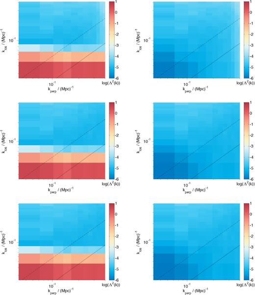
We first construct cylindrical power spectrum for the different signal contributions in order to understand how the EoR window is constructed. In Fig. 1, we see the Galactic synchrotron, Galactic free–free and unresolved extragalactic foregrounds while in Fig. 2 we see the dirty cosmological signal and dirty foregrounds (with all three foreground contributions summed). The action of the PSF can be clearly seen as a loss of power on scales above this (i.e. for kperp > 0.65 Mpc−1). Note that, since we are seeing power spectrum over a 10 MHz bandwidth only we do not see the evolution of the cosmological signal over redshift. We see clearly the area of k-space where the foregrounds appear to be at their strongest is at low klos, however, it should be noted that there is appreciable foreground contamination across a large proportion of the plane. The cosmological signal has clear contours with the strongest signal at low k – right beneath the foreground contamination. By choosing to avoid the foregrounds we will implicitly lose information on the strongest part of the cosmological signal.
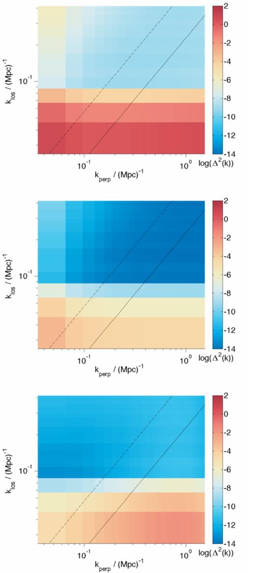
The cylindrical power spectrum for the Galactic synchrotron, Galactic free–free and extragalactic foregrounds (from top to bottom). This is for a 10 MHz bandwidth centred at 165 MHz. The theoretical wedge limit line is shown in black.
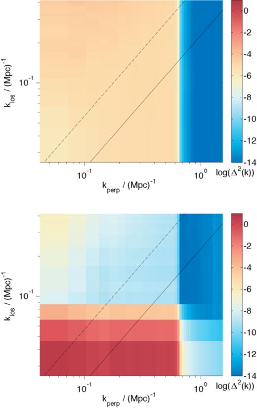
The cylindrical power spectrum for the cosmological signal (top) and combined foregrounds (bottom, i.e. sum of Galactic synchrotron, Galactic free–free and extragalactic foregrounds) both convolved with a LOFAR 115 MHz PSF.
5.1 Choice of window function
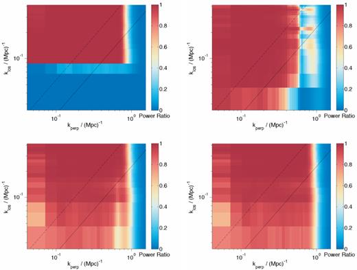
The cylindrical power spectrum are calculated by first applying a window function along the line of sight in order to suppress the sidelobes associated with the Fourier transformation of a finite signal. The choice of this window is not unimportant as different windows can cause different levels of foreground suppression to be balanced with less sensitivity (Vedantham et al. 2012; Thyagarajan et al. 2013). We compare the cleanliness of the EoR window for four different types of window, rectangular, Hanning, Blackmann–Nuttal and extended Blackman–Nuttall (the forms of which are shown in Fig. 3) in Fig. 4.
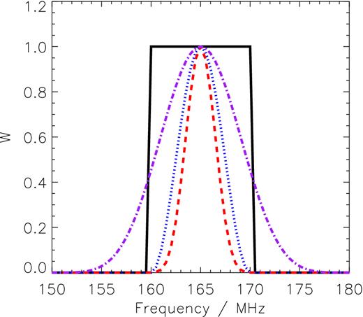
The 10 MHz rectangular (black, solid), Hanning (blue, dot), Blackmann–Nuttall (red, dash) and extended Blackman–Nuttall (purple, dash-dot) window.
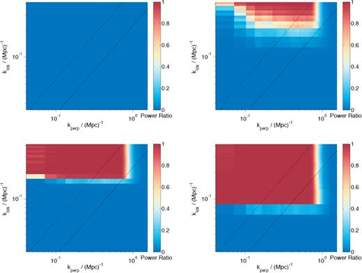
The ratio of cs/cs + fg for a 10 MHz rectangular, Hanning, Blackmann–Nuttall and extended Blackman–Nuttall window (in reading order). The extended Blackmann–Nuttall provides the largest clean window. The lines represent theoretical wedge contamination limits for sources contributing from within the field of view of 10 deg (dashed) and from within the FWHM of the station beam (dotted).
It is clear that different windows result in different suppression of the foreground contamination of the EoR window. The extended Blackman–Nuttall window seems to result in the most clean window and for all results following we choose to use the extended Blackmann–Nuttall window.
5.2 Smooth foreground models
We can take a first look at the power spectrum recovery of the two methods by looking at the cylindrical power spectrum of Fig. 5. We do this for three scenarios. The first, S1, with the LOFAR 600 h noise as described above. The second, S2, we divide our noise by 10 in an approximation to the expected SKA noise. Finally, we look at the ‘perfect’ situation where there is zero instrumental noise in an effort to understand the foreground effects alone, S3. We can clearly see the dominant foreground contribution in red at low klos for all three scenarios. For all scenarios, we can see the contours which were apparent in the cosmological signal plot.
The cylindrical power spectrum for the three scenarios, S1, S2 and S3 from top to bottom. In the left-hand column is the total input signal for each scenario (i.e. the data for foreground avoidance) while on the right hand is the residual as produced by GMCA for each scenario (i.e. the data after foreground removal). Linestyles are as in Fig. 4.
In order to visualize the results of using the EoR window approach and foreground removal we ran the total input signal cube through GMCA assuming four components in the foreground model. In the remaining three panels of Fig. 5, we present the cylindrical power spectrum of the three residuals cubes. It is clear that GMCA is able to remove the foreground contamination very well, though whether it affects the cosmological signal as a result of inaccurate foreground modelling is less clear.
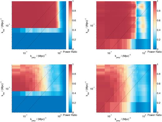
In order to assess the accuracy of the foreground removal across the k-plane, we calculate the foreground fitting errors which are the difference between the simulated foregrounds and those modelled by GMCA. We display the ratio |$\frac{cs}{\mathrm{cs}+\mathrm{fg_{fitterr}}}$| for each scenario in Fig. 6. While, as stated before, direct comparison between foreground removal and foreground avoidance on data without action of a frequency dependent PSF should be treated with some caution, we can see how the methods work differently. We first of all see that with expected LOFAR noise we are able to recover a much greater portion of the window at klos < 0.09 i.e. GMCA is successfully removing the foregrounds. We note however that compared to foreground avoidance less of the window is recovered at kperp > 0.4 Mpc−1. This is due to the noise confusing the GMCA method and resulting in a less accurate foreground model. As we reduce the noise in S2 we see a similar range of kperp is recovered as foreground avoidance and for the ideal no-noise S3 we have almost the entire window recovered, barring the PSF action at kperp > 0.6 Mpc−1. This is a most promising result for both methods as we see large portions of the window recovered. For current generation telescopes it may be that a combination of the methods proves most fruitful in order to access as much of the window as possible. If the desire is for as much good quality data as possible irrespective of scale, foreground avoidance will be useful. On the other hand, to access those smallest klos scales, foreground removal will be necessary. If the action of a frequency dependence PSF can be successfully mitigated then by the time the next generation data is available it seems that foreground avoidance will provide little advantage over foreground removal.
In reading order: the ratio cs/(fg + cs) which relates to the foreground avoidance method assuming perfect noise knowledge. The ratios cs/(fgfiterr + cs) for the three scenarios, S1, S2 and S3, which relate to the foreground removal method assuming perfect noise knowledge. If the ratio plot is equal to one then foreground contamination is nil. Linestyles are as in Fig. 4.
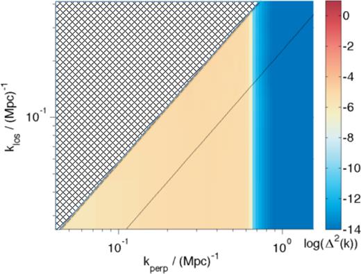
A cartoon to show how we define the recoverable EoR window in our quantitative calculation. The hashed area represents the total EoR window (WFoV) which we consider recoverable if using the field-of-view wedge line. If all cells in this area were successfully recovered, we would deem the proportion of the window recovered to be 100 per cent. WBeam is defined as the region extending to the solid wedge line.
In Fig. 8 we see that the level of signal-to-noise recovered is dependent both on frequency and on the level of noise, as expected. We see that for the LOFAR scenario (red lines), foreground removal results in a slightly higher signal-to-noise ratio across the frequency range. In the lowest frequency bins the signal-to-noise ratio decreases significantly for foreground avoidance. This is because the cosmological signal decreases significantly at these frequencies and so the signal-to-foreground level is severely diminished. In contrast, foreground removal methods are able to remove the foregrounds in order to recover an improved signal-to-noise even very low signal-to-foreground levels. For the SKA scenario (black lines) we see the same trends, except that above 160 MHz, the signal-to-noise for foreground removal decreases slightly below the foreground avoidance line. This suggests that the foreground fitting errors are the dominate source of noise on the signal at these frequencies - not the noise or foregrounds themselves. This suggests that for the next generation of telescopes further optimisation of the foreground removal codes may be necessary. As pointed out before, a direct comparison is not completely robust without proper frequency dependence of the PSF and the SN does not take into account that if one were to desire only scales within the range 0.4 < kperp < 0.6 for example, then it would be best to choose foreground avoidance.

5.3 Less smooth foreground models
The assumption of smooth foregrounds such as those modelled in this paper is key to the success of many parametric and some non-parametric (e.g. Harker et al. 2009) foreground removal methods. In this section, we assess the degree to which foreground avoidance and removal can be compromised by relaxing this assumption. We investigate four possibilities. First, we adjust each slice of our clean foreground simulation by multiplying with a random number drawn from a Gaussian distribution with standard deviation of 0.01. This very roughly models an inherent 1 per cent variation of the foreground magnitude along the line of sight. We then do the same but with a standard deviation of 0.001 to create a 0.1 per cent variation scenario. We see the results of applying the methods to total signal cubes made with these adjusted foreground cubes in Fig. 9. We run GMCA on the data cubes including LOFAR-like instrumental noise and so the resulting ratios can be directly compared to the top panels of Fig. 6. We see that neither cube is too adversely affected by the 0.1 per cent variation, though the foreground avoidance method does suffer some degradation at kperp < 0.2 Mpc−1 due to the small-scale wiggle introducing structure into the foregrounds which cannot be confined purely in a band at low klos. However, for 1 per cent variation we see a marked difference. While GMCA is still able to model to foregrounds quite accurately for kperp < 0.6 Mpc−1, the EoR window for foreground avoidance is much obscured. This is an important drawback of foreground avoidance to note. While there is little argument that the physical processes producing much of the foregrounds result in a smooth frequency dependence, it is not clear how the instrumentation and data reduction pipeline might encroach on this smoothness. Blind methods such as GMCA provide a clear advantage in such a case, as no assumption of smoothness is made. In contrast, for foreground avoidance to work it must assume the foregrounds are confined to within a clear low klos area. If in the case of a significant LOS variation this assumption fails and the foreground contamination within the EoR window is too high. Note that we present the ‘best-case’ for foreground removal here – where the frequency dependence of the PSF has been perfectly mitigated.

In the left-hand column, we show the ratio cs/cs+fg for the 0.1 and 1 per cent LOS varying foreground models (top and bottom, respectively). In the right-hand column, we show the same ratio but with the foreground fitting errors as a result of performing GMCA on the new foreground cubes with LOFAR noise. We see that foreground avoidance is affected badly by introducing a 1 per cent LOS variation, while GMCA is still able to make a good recovery, under the assumption of common resolution channels. Linestyles are as in Fig. 4.
Next we make the adjustment to the foregrounds spatially varying by multiplying every pixel by a random number as described above. This is in addition to the LOS variation. This emulates some form of instrumental calibration error such as leakage of polarized foreground from the Stokes Q and U channels to the Stokes I channel. In Fig. 10 we see that even with both spatial and LOS 0.1 per cent variation, there is no reduction in the quality of recovery for either method. However, once this variation is increased to 1 per cent GMCA shows a marked decrease in accuracy in its foreground model and recovery across the whole k range, though especially at kperp > 0.3, where the small-scale spatial wiggle is at its most significant. This is intriguing as it gives us insight into how GMCA uses sparsity to define the foreground components. While the smoothness of the foregrounds may aid GMCA in finding a basis in which a foreground component can be considered sparse, it is apparent from these results that it is not this smoothness which is essential for the method to work. However, once the spatial variation is included, GMCA fails to model the foreground accurately, indicating that it is the spatial correlation of the foregrounds which enables GMCA to find a sparse description of the foreground signal. Interestingly foreground avoidance actually seems to do a better job than with LOS variation alone. We believe that this is because the introduction of a spatial variation softens the variation along the line of sight somewhat, confining the foregrounds once again to a low klos area. This could be a quirk of our particular simulations of the variations however and may warrant further investigation.
In the left-hand column, we show the ratio cs/cs+fg for the 0.1 and 1 per cent (top and bottom, respectively) LOS+spatial varying foreground models. In the right-hand column, we show the same ratio but with the foreground fitting errors as a result of performing GMCA on the new foreground cubes with LOFAR noise. While GMCA is able to cope fairly well with a 0.1 per cent variation, the 1 per cent LOS+spatial variation results in a dramatic reduction in recovery across the k range. Linestyles are as in Fig. 4.
We note that the foreground models here are not an attempt to model specific instrumental or physical effects. We intend to explore a fully physically motivated foreground leakage model in further work and simply present the toy models here as a first step to understanding the sensitivity of the methods to non-smooth foreground models. To truly assess the ability for GMCA to model the extra degrees of freedom introduced by a non-smooth foreground model would require a Bayesian model selection algorithm in order to select for the model with the most likely number of foreground components. The results presented here are in fact a non-optimal presentation of GMCA in this respect as we have not changed the number of components used by GMCA to model the non-smooth foregrounds. We leave the development of a Bayesian model selection algorithm and resulting analysis to further work.
6 CONCLUSIONS
This paper set out to consider the loss of sensitivity in the power spectrum recovery using foreground avoidance, while also presenting how a foreground removal method currently adopted in EoR pipeline preserved that sensitivity in the optimal case of common resolution channels. This is a timely investigation due to the current data analysis being carried out by several major radio telescope teams around the globe in order to uncover the cosmological signal for the first time. Being a first detection of a rather unconstrained entity, we need to be confident in our methods for recovering it and understand how different methods might produce different results.
We aimed to begin to understand this by applying both techniques to three sets of simulations: one with LOFAR level noise, one with SKA level noise and one with no noise at all. The comparison was an extremely fruitful one and very promising with respects to both methods. We did however ascertain several differences between the methods:
While the omission of low klos scales in foreground avoidance undoubtedly prevents foreground removal bias within the remaining signal, the amount of cosmological signal at those same omitted scales is not negligible. This could have a serious impact on investigations of, for example, redshift space distortions, as pointed out in Pober (2015).
Pursuing foreground removal results in a more complete reconstruction at low klos however there is a worse recovery at kperp > 0.6 Mpc−1 due to foreground fitting errors. This is due to the noise confusing GMCA. The recovery improves as we go to lower noise scenarios, with the no-noise scenario recovering the same range of kperp scales as foreground avoidance.
Quantifying the amount of signal recovered in the EoR window, we find that foreground removal recovers a greater signal-to-noise ratio than foreground avoidance across the frequency range for the LOFAR scenario. While for the SKA scenario, both methods recover a greater signal-to-noise, as expected, foreground removal does appear to overfit the foregrounds at the higher frequencies when all scales are considered and this needs to be investigated further. It may be that at SKA noise levels the number of components in the foreground model needs to be more carefully chosen to avoid over-fitting.
Neither foreground avoidance or foreground removal is too adversely affected by a LOS or spatial variation of 0.1 per cent.
When a LOS-only variation of 1 per cent is introduced we see that while GMCA can still recover the cosmological signal to the same degree, the EoR window is far too obscured for foreground avoidance to be an effective method.
For a spatial and LOS variation of 1 per cent, GMCA is diminished in its accuracy however can still recover a reasonable area at low kperp and still a larger area than foreground avoidance. Interestingly foreground avoidance seems to do better with spatial and LOS variation than with the LOS variation alone. We believe this to be as a result of the spatial variation diminishing the LOS variation by chance.
At current generation noise levels it would probably be advantageous to use both methods in order to recover as much of the window as possible. However once we reach next generation noise levels the advantage of using foreground avoidance is less clear assuming the satisfactory mitigation of the frequency dependent PSF.
This was a basic first look at the loss of sensitivity invoked by both methods and there is still much work to be done. The frequency dependence of the PSF is a known issue with respects to the cleanliness of the EoR window above the wedge due to mode mixing. While for this first attempt we enforced a common resolution motivated by the recent results of a successful weighting scheme, we will need to consider how this frequency dependence can be mitigated by both methods in order to provide an equal footing comparison. We also would like to consider the wedge in more detail by including bright point sources in our analysis and modelling their inaccurate removal.
EC acknowledges the support of the Royal Astronomical Society via a RAS Research Fellowship. EC would like to thank Ajinkya Patil, Cathryn Trott, Jonathan Pritchard, Geraint Harker and Harish Vedantham for useful discussions. FBA acknowledges the support of the Royal Society via a University Research Fellowship. VJ would like to thank the Netherlands Foundation for Scientific Research (NWO) for financial support through VENI grant 639.041.336. The work involving oskar was performed using the Darwin Supercomputer of the University of Cambridge High Performance Computing Service (http://www.hpc.cam.ac.uk/), provided by Dell Inc. using Strategic Research Infrastructure Funding from the Higher Education Funding Council for England and funding from the Science and Technology Facilities Council.
REFERENCES
