


Abstract
With ALMA (Atacama Large Millimeter/submillimeter Array) making it possible to resolve giant molecular clouds (GMCs) in other galaxies, it is becoming necessary to quantify the observational bias on measured GMC properties. Using a hydrodynamical simulation of a barred spiral galaxy, we compared the physical properties of GMCs formed in position–position–position (PPP) space to the observational position–position–velocity (PPV) space. We assessed the effect of disc inclination: face-on (PPVface) and edge-on (PPVedge), and resolution: 1.5 pc versus 24 pc, on GMC properties and the further implications of using Larson's scaling relations for mass–radius and velocity dispersion–radius. The low-resolution PPV data are generated by simulating ALMA Cycle 3 observations using the casa package. Results show that the median properties do not differ strongly between PPP and PPVface under both resolutions, but PPVedge clouds deviate from these two. The differences become magnified when switching to the lower, but more realistic resolution. The discrepancy can lead to opposite results for the virial parameter's measure of gravitational binding, and therefore the dynamical state of the clouds. The power-law indices for the two Larson's scaling relations decrease going from PPP, PPVedge to PPVface and decrease from high to low resolutions. We conclude that the relations are not entirely driven by the underlying physical origin and therefore have to be used with caution when considering the environmental dependence, dynamical state, and the extragalactic CO-to-H2 conversion factor of GMCs.
1 INTRODUCTION
As many observations show that star formation efficiency varies by ∼100 times from galaxy to galaxy, increasing attention has been devoted to the questions of whether giant molecular cloud (GMC) properties are universal and whether their star formation ability depends on the large-scale galactic environment. The Atacama Large Millimeter/submillimeter Array (ALMA) observations are starting to resolve a wide population of GMCs with the quality of that in the Milky Way. This gives a chance to reveal the whole picture of the relation between GMCs and star formation in various environments. To interpret the measured GMC properties properly, it is necessary to understand any observational bias on the GMC properties.
It is still debated if the physical properties of continuous structure in the interstellar medium (ISM) measured by spectral line observations (e.g. 12CO, HCN) represent the intrinsic structures in three dimensions (e.g. Adler & Roberts 1992; Pichardo et al. 2000; Ostriker, Stone & Gammie 2001; Sheth et al. 2008; Shetty et al. 2010; Ward et al. 2012; Beaumont et al. 2013; Pan et al. 2015). Observations take data from the galaxies projected on the sky plane. This provides two spatial dimensions (RA and Dec.) and a velocity along the line of sight (LOS), known as the spectral data cube in position–position–velocity (PPV) space. However, the non-spherical shapes of GMCs change their appearances when projected along different LOS, which are determined by the inclination and position angle of the host galactic disc. Moreover, galaxies are distributed over a wide range in distance in the Universe, causing the physical resolution of observations to not always be the same. Finite resolution will necessarily introduce contributions from separated adjacent structures to the measured GMC properties.
These effects are assessable by comparing GMC properties in observations to simulations. Simulations normally have data with three-dimensional position (x, y, z) and velocity (vx, vy, vz) coordinates, so-called position–position–position (PPP) space, from which GMC properties can be directly calculated. In previous work, we compared the physical properties of the GMCs identified in PPP and those in PPV in the same simulated galaxy, assuming ideal circumstances, i.e. face-on observation with high resolution (1.5 pc) and sensitivity (1 K per 1 km s−1; Pan et al. 2015). The results show that PPP and PPV can potentially identify the same objects with closely matched properties within a scattering in value of a factor of 2. Yet such high resolution and sensitivity are very difficult to achieve in extragalactic observations even with ALMA.
In this work, we further evaluate the effects of galactic disc inclination and observed resolution. As in Pan et al. (2015), this is done by comparing GMCs in PPP and PPV. This paper is organized as follows. Method and data sets are introduced in Section 2. The cloud identification methods and the derivation of physical properties are introduced in Section 3. Section 4 presents the results of this work. We summarize the key results of our analysis in Section 5.
2 METHOD AND DATA SETS
The simulated galaxies were modelled on the barred spiral (SABc) galaxy, M83, using observational data from the 2MASS K-band image to estimate the stellar potential. The simulations were run using the three-dimensional adaptive mesh refinement (AMR) hydrodynamics code, enzo (Bryan et al. 2014). The high-resolution (1.5 pc) simulation is presented in Fujimoto et al. (2014), along with a full description of the run parameters. The gas radiatively cooled down to 300 K but no star formation or feedback was included. Typical temperatures in the GMCs are about 10 K, an order of magnitude below our minimum radiative cooling temperature. However, our resolution is not sufficient to resolve the full turbulent structure of the gas, and we also do not include pressure from magnetic fields. Including a temperature floor of 300 K therefore imposes a minimum sound speed of 1.8 km s−1 on the gas to crudely allow for these effects. The velocity dispersion within our GMCs is typically higher than this by about a factor of 2–3, implying that this floor does not have a significant impact on the cloud properties. Previous work that has compared runs with and without star formation and feedback physics suggest that GMC properties are not strongly affected by these additions. We have therefore not included a star formation model in this work, focusing on the properties of the gas (Tasker & Tan 2009; Tasker 2011; Tasker, Wadsley & Pudritz 2015).
Face-on and edge-on projection images of the high-resolution simulated galaxy are shown in the bottom and top panels of Fig. 2(a). To assess the resolution effect, a low-resolution (24 pc) simulation was made by decreasing the total levels of refinement. The remaining run parameters are the same as in the high-resolution simulation.
There are six data sets in total, summarized in Table 1. Data structure of PPP, edge-on observation in PPV, and face-on observation in PPV are prepared. Each data set is produced at two resolutions: 1.5 pc (with 1 km s−1 for PPV velocity axis) and ∼24 pc (with 2 km s−1). The high- and low-resolution PPP data using the aforementioned two simulations are presented as PPPH and PPPL, respectively.
Summary of the data sets in this work.
| 3D clouds | Edge-on observations | Face-on observations | ||||
|---|---|---|---|---|---|---|
| PPPH | PPPL | PPV|$\mathrm{_{edge}^{H}}$| | PPV|$\mathrm{_{edge}^{L}}$| | PPV|$\mathrm{_{face}^{H}}$| | PPV|$\mathrm{_{face}^{L}}$| | |
| Data set final resolution (pc) | 1.5 | 24 | 1.5a | ∼24b | 1.5 | ∼24 |
| Resolution of simulation (pc) | 1.5 | 24 | 1.5 | 1.5 | 1.5 | 1.5 |
| PPV convolved by CASA | – | – | N | Y | N | Y |
| Representation of resolution | AMR level | AMR level | Pixel size (MW- | Beam size from casa | Pixel size (MW- | Beam size from casa |
| of simulation | of simulation | and LG-like obs.c) | (extragalactic obs.) | and LG-like obs.) | (extragalactic obs.) | |
| Note | Pan et al. (2015)d | – | – | Assume ALMA obs.e | Pan et al. (2015) | Assume ALMA obs. |
aWe use PPVH to denote ‘PPV|$\mathrm{_{edge}^{H}}$| and PPV|$\mathrm{_{face}^{H}}$|’.
bWe use PPVL to denote ‘PPV|$\mathrm{_{edge}^{L}}$| and PPV|$\mathrm{_{face}^{L}}$|’.
cMW: Milky Way; LG: Local Group.
dDetailed comparison of PPPH and PPV|$\mathrm{_{face}^{H}}$| is shown in Pan et al. (2015).
ecasa can generate the visibilities measured with ALMA, VLA, CARMA, SMA, and PdBI. ALMA is chosen for this work.
The LOS of PPV data is the z-axis for the face-on case, and y-axis for the edge-on case. The chosen resolutions will return clouds with fully and barely resolved properties respectively if the simulated clouds have properties similar to the Galactic GMCs. Velocity resolutions are chosen so that the smallest clouds in both spatial resolutions can span across two to three velocity channels if following the Larson's relation (cf. Section 4.3).
The high-resolution PPV data are created from the high-resolution (1.5 pc) simulation. The pixel size matches to cell size at 1.5 pc. When identifying GMCs in the PPV data set, we assume that the galaxy is observed in 12CO (1–0) (115.2 GHz), the most commonly used transition for GMC observations. Therefore, only cells with a density greater than 100 cm−3 were included in the data, corresponding to the excitation density of 12CO (1–0). This is consistent with the cloud identification of the PPP clouds, which selected using a continuous contour at a density of 100 cm−3. The cloud identification algorithm of PPV expects the data to be emission intensity, rather than the gas density followed by simulations. We use a Galactic CO-to-H2 conversion factor (XCO) of 2 × 1020 cm−2 (K km s−1)−1 (Bolatto, Wolfire & Leroy 2013) to convert between the two. Since we do not consider chemistry nor radiative transfer and the excitation of molecular lines, the conversion factor cancels when we derive the cloud mass, so its precise value does not affect our results. This also means that we have a more accurate mass measurement than real observations, and this work is thus an assessment purely for the unavoidable effects of projection, resolution, sensitivity and cloud identification method in observations, i.e. any discrepancy between the data sets can be largely attributed to these effects. The high-resolution face-on and edge-on PPV data are referred to as PPV|$\mathrm{_{face}^{H}}$| and PPV|$\mathrm{_{edge}^{H}}$|, respectively. Comparisons between PPPH and PPV|$\mathrm{_{face}^{H}}$| have been presented in Pan et al. (2015).
In observations, the image is formed by convolving the intrinsic structures of the observed target with a two-dimensional Gaussian ‘beam’. The convolution plays a critical role in determining the appearance of the GMCs when the beam size is ≥ GMC size. To reproduce the convolution in the low-resolution PPV, the Common Astronomy Software Applications (casa) package (McMullin et al. 2007) is used to simulate ALMA Cycle 3 (2015 October–2016 September) 12CO (1–0) observations. The input sky model is the noise-free PPV|$\mathrm{_{edge}^{H}}$| and PPV|$\mathrm{_{face}^{H}}$| in unit of flux corrected by the XCO, assuming a distance and coordinate of M83. Therefore, all of PPV data sets are created from the simulation with 1.5 pc resolution. casa task simobserve is used to construct the uv visibilities for the specified antenna configuration, then simanalyze is used to Fourier transform the uv visibilities into the image plane. Hexagonal mosaic is adopted for mapping. The observing time of 12 m array is about 1 min on each mosaic pointing. The baselines range from 14.7 to 538.9 m. Note that we only use the 12 m array, and the effect of interferometric observation, e.g. short-spacing problem, is kept as part of the comparison because most of extragalactic observations did not have corresponding single-dish observation to combine. Around 60 per cent of the total flux (estimated from the noise-free PPVH) are missed. The observation is only sensitive to structures <500 pc, but is large enough to detect the GMC-scale structures. The final resolutions of the low-resolution PPV (PPV|$\mathrm{_{edge}^{L}}$| and PPV|$\mathrm{_{face}^{L}}$|) are ∼24 pc (∼1.3 arcsec) and 2 km s−1. The rms noise level (σrms) is ∼10 mJy (∼0.55 K), leading to a typical mass sensitivity (1σrms in 1 channel) of 2 × 10³ M⊙.
This observation setup is comparable to several ongoing ALMA projects on nearby galaxies. In Fig. 1, we present a side-by-side showcase of how the ALMA processing affects the data. Panels (a) and (b) show an ∼700 pc area seen in PPV|$\mathrm{_{face}^{H}}$| and PPV|$\mathrm{_{face}^{L}}$|, respectively. Comparison of two figures shows that small clouds in the high-resolution data disappear in the low-resolution data because of the lower resolution or/and sensitivity. Moreover, clouds become more spherical in panel (b) due to the image convolution with the circular beam.
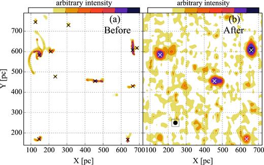
An example of how the ALMA processing affects the data. Panels (a) and (b) show an ∼700 pc area of the face-on galaxy observed with high and low resolutions (PPV|$\mathrm{_{face}^{H}}$| and PPV|$\mathrm{_{face}^{L}}$|), respectively. Beam size (∼24 pc) of low resolution is shown in panel (b) with black filled circle. Centres of mass of GMCs are marked with black or white crosses. It is clear that because of the low resolution or/and sensitivity in our setup, the small clouds in the high-resolution data disappear in the low-resolution data. Moreover, clouds become more spherical in panel (b) due to the image convolution with the circular beam.
3 DEFINITION OF CLOUDS IN SIMULATION AND OBSERVATION
The cloud identification methods are identical to Pan et al. (2015). In both data structures, GMCs are identified as continuous structures of gas above a chosen density or flux threshold, and multiple peaks are allowed within a GMC. This method, which we refer to as the island method in Pan et al. (2015), is the better choice for selecting similar objects between simulation and observation data structures, compared to the decomposition method which further segregates the peaks within an island into individual clouds.
PPP works from the lowest density, drawing a contour at |$n_{{\rm H\,\small {I}, thresh}} = 100$| cm−3 and defining all cells within a closed section as the cloud (Fujimoto et al. 2014). PPV clouds are identified using cprops (Rosolowsky & Leroy 2006). The package was designed to identify continuous structures in the observed spectral data cube. cprops begins by masking the emission with a high signal-to-noise ratio (S/N; 4 × rms noise in this work), picking out the cloud locations at densities much higher than the background. It then extends this mask to the user-defined lowest S/N (2 × rms noise in this work), which outlines the observed cloud boundary. cprops then assumes that the real cloud boundary is larger than the observed cloud boundary, since the cloud outer regions are being obscured by the background noise. It therefore extrapolates linearly from the observed boundary to a sensitivity of 0 K to form the real cloud boundary.
Physical properties of the clouds are derived once the cloud boundaries are set. Derivations of physical properties in PPP and PPV have been fully described in Fujimoto et al. (2014) and Rosolowsky & Leroy (2006), respectively. In this section, we provide a brief qualitative summary. These derivations are not identical between the two methods, since the raw data measure different quantities in different data structures. We do not correct for this, but adopt the original calculations as part of the comparison.
In both data structures, cloud mass is a direct measured property from the sum of cells or pixels enclosed within the cloud boundary. Radius and velocity dispersion of PPP clouds are calculated from three spatial and three velocity dimensions. For cloud radius, the average radius of the cloud is measured from its projected area in the x–y, x–z, and y–z planes. The mass-weighted one-dimensional velocity dispersion of PPP clouds is computed from the average deviations between the gas velocity and the cloud bulk velocity in x, y, and z direction. PPV, however, must measure the mass(flux)-weighted projected radius at the plane perpendicular to the LOS (note that PPP does not consider any weighting in deriving radius) and the mass(flux)-weighted velocity dispersion along the LOS using the second moments of the emission along the spatial and spectral axes.
The derived cloud properties, which depend on multiple cloud variables, are calculated from the three basic properties above. Surface density, Σc, is defined as the mass per unit area and is simply calculated from the cloud mass and radius. Virial parameter, αvir, measures the gravitational binding of a GMC, assuming a spherical profile and no magnetic support or pressure confinement. The classic derivation is defined as the ratio of virial mass (Mvir) to cloud mass (Mc) as αvir ≈ Mvir/Mc, where Mvir is calculated from the cloud radius (Rc) and velocity dispersion (σc) as Mvir ≈ 1040 Rc σc2. αvir > 2 indicates that the cloud is gravitationally unbound while αvir < 2 are bound clouds (Bertoldi & McKee 1992).
4 RESULTS
4.1 Physical properties of the GMCs in the high-resolution analysis
The probability distribution functions of the high-resolution cloud properties are shown in the upper panels of Figs 2(b)–(f). Green solid, red dashed, and blue dotted curves represent PPPH, PPV|$\mathrm{_{edge}^{H}}$|, and PPV|$\mathrm{_{face}^{H}}$|, respectively. The coloured vertical lines indicate the median value of the properties for each data set.
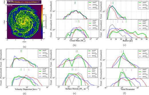
(a) Edge-on (top) and face-on (bottom) projection images of the simulated galaxy in high resolution. (b) Normalized distribution of cloud mass in high (top) and low (bottom) resolutions. Green solid, red dashed, and blue dotted curves denote the distribution of PPP, PPVedge, and PPVface, respectively. In the bottom plots, we overlay the distribution of the high-resolution PPP clouds (the green curves in the upper panels) with gray curves to compare since it represents the ‘real’ case. The coloured vertical lines denote the median value of each parameter. (c) Radius. (d) Velocity dispersion. (e) Surface density. (f) Virial parameter with the same segregation for both resolutions.
The median value of the cloud mass is consistent between the three data sets at ∼3 × 10⁵ M⊙, but shapes of the profiles slightly differ. PPPH and PPV|$\mathrm{_{face}^{H}}$| have almost identical mass profile. Pan et al. (2015) found that as high as 70 per cent of clouds have single counterpart in both data structures with a mass difference of <50 per cent.
The blending effect is evident for PPV|$\mathrm{_{edge}^{H}}$| as demonstrated in Fig. 3(a). The figure shows the galactocentric distribution of cloud numbers. Line styles and colours are the same as in the 1D profiles. Galactocentric distances (Rg) of PPPH and PPV|$\mathrm{_{face}^{H}}$| are calculated by their 3D and 2D position, respectively. PPV|$\mathrm{_{edge}^{H}}$|, however, must use the kinematic distance. If LOS velocities are known, clouds at a particular velocity can be assigned a position along the LOS, and thus a particular Rg. The method introduced by Yim et al. (2011) is adopted for this. All three data structures detect two concentrations of clouds at radii Rg ≈ 2–3 kpc and Rg ≈ 6–7 kpc, corresponding to the radii of the galactic bar and the spiral arms. However, the number of clouds in PPV|$\mathrm{_{edge}^{H}}$| lies below both the PPPH and PPV|$\mathrm{_{face}^{H}}$| cases by ∼2 times, indicating the cloud blending. Therefore, even though the range and profile of the cloud mass in PPV|$\mathrm{_{edge}^{H}}$| do not deviate significantly from that of PPPH and PPV|$\mathrm{_{face}^{H}}$| overall, this should not lead to the interpretation that the cloud masses between the three data sets are the same.
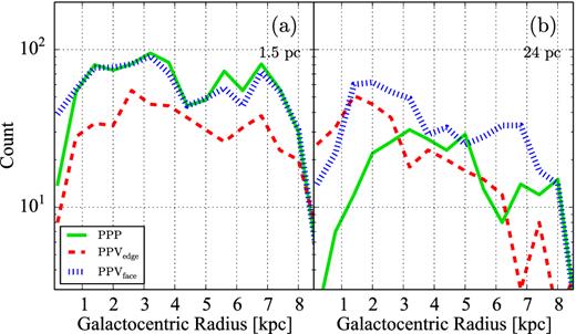
Galactocentric distribution of cloud numbers in (a) high and (b) low resolutions. Green solid, red dashed, and blue dotted curves represent the clouds from PPP, PPVedge, and PPVface, respectively. Galactocentric distances of PPP and PPVface are calculated by three- and two-dimensional position, respectively, while PPVedge adopts kinematic distance using the method introduced in Yim et al. (2011). In the high resolution, the cloud numbers are similar across all data sets, showing two concentrations at the radii of galactic bar and spiral arms. However, the cloud number of PPV|$\mathrm{_{edge}^{H}}$| lies below PPPH and PPV|$\mathrm{_{face}^{H}}$| by roughly a factor of 2, indicating the cloud blending. In the low resolution, PPV|$\mathrm{_{edge}^{L}}$| no longer represent the intrinsic distribution of clouds, but decline with radius, whereas PPV|$\mathrm{_{face}^{L}}$| show a similar profile as PPPL and their high-resolution counterparts, but with fewer clouds everywhere.
The cloud radii identified in PPV|$\mathrm{_{edge}^{H}}$| are smaller compared to the other two data sets (Fig. 2c). This is due to the flat galactic disc (Fig. 2a), and is visualized in Fig. 4. Figs 4(a) and (b) show the slice plots of a 400 pc patch of PPV|$\mathrm{_{face}^{H}}$| and PPV|$\mathrm{_{edge}^{H}}$|, respectively, and the corresponding projection plots in panels (c) and (d). Only the cells with density >100 cm−3 are plotted; therefore, most of the coloured regions have been assigned to clouds. It can be seen from panel (b) that clouds are flat in the z-axis, and consequently, the slice and projection plots of PPV|$\mathrm{_{face}^{H}}$| [panels (a) and (c)] show higher similarity and less crowding due to the small depth of the LOS, and vice versa for panels (b) and (d). The gas scaleheight of our simulated galaxy is about 80–115 pc, which is similar to the initial value of 100 pc due to the lack of stellar feedback to inject energy; nevertheless, recent observations of edge-on spiral galaxies show that the scaleheights of molecular gas traced by 12CO (1–0) are mostly <150 pc (Yim et al. 2011, 2014), so this effect replicates true observations as well. The velocity dispersion shows very little difference between PPVedge and PPPH/PPV|$\mathrm{_{face}^{H}}$| (Fig. 2d). All of methods suggest a median value of ∼5 km s−1.
![Example of GMCs seen from different viewing angles of z-axis (face-on, left) and y-axis (edge-on, right). Note that y-axis ticks of the edge-on cases [panels (b) and (d)] are shown at the right-hand side. Only the cells with density >100 cm−3 are plotted; therefore, most of the coloured regions have been assigned to clouds. Panels (a) and (b) present the slice plots of face-on and edge-on views, respectively; panels (c) and (d) show projection plots of the same orientations. The representative region is located at the spiral arm with galactocentric radius of ∼6 kpc. It can be seen from panel (b) that clouds are flat in the z-axis, and consequently, the slice and projection plots of PPV$\mathrm{_{face}^{H}}$ [panels (a) and (c)] show higher similarity and less crowding due to the small depth of the LOS, and vice versa for panels (b) and (d).](https://oup.silverchair-cdn.com/oup/backfile/Content_public/Journal/mnras/458/3/10.1093_mnras_stw478/2/m_stw478fig4.jpeg?Expires=1749848557&Signature=17xCmQ~5WQzDMlIeoZLYLYYscurBRHu7NgOEqwnL7bN-6EhjAyEgjmxLDbbDNF5YDYRC4QdnSe9asPBqBZuyjhd4Wmic28qCxRBAM8KATQkmJoipBcH5fMiL9tdj8jmq0DxVJPkIdSCSwqkOnHF64RnU4wegv~4ja~v4n3Ja1tiM6OAWdsEiar5F4DMxvGc0kGWJLAEyv-D2yBeGgPxfC1cpqKbJ9pCcXKXRupNJhmI2YUy-5q0Megedja3~EYcJzKFT-0Rnts7hGNlocyRSsX3Xre-sV7ULJo8u0ho2KK0IsCurD2rYl9CHefzRzhRqWFKbMJUE6PGA7IjcPPpOeg__&Key-Pair-Id=APKAIE5G5CRDK6RD3PGA)
Example of GMCs seen from different viewing angles of z-axis (face-on, left) and y-axis (edge-on, right). Note that y-axis ticks of the edge-on cases [panels (b) and (d)] are shown at the right-hand side. Only the cells with density >100 cm−3 are plotted; therefore, most of the coloured regions have been assigned to clouds. Panels (a) and (b) present the slice plots of face-on and edge-on views, respectively; panels (c) and (d) show projection plots of the same orientations. The representative region is located at the spiral arm with galactocentric radius of ∼6 kpc. It can be seen from panel (b) that clouds are flat in the z-axis, and consequently, the slice and projection plots of PPV|$\mathrm{_{face}^{H}}$| [panels (a) and (c)] show higher similarity and less crowding due to the small depth of the LOS, and vice versa for panels (b) and (d).
In the analysis of this simulation using the same cloud identification method, Fujimoto et al. (2014) found that PPPH clouds fall into three populations: the most common ‘Type A’ clouds, with properties that corresponded to the average values measured in observations, the ‘Type B’ massive GMC associations that formed during repeated mergers of smaller clouds, and the transient ‘Type C’ that were born in tidal tails and filaments. The three types result in the bimodal distribution of cloud surface density (Σc) at ∼1000 M⊙ pc−2 (‘Type A’ and ‘Type B’) and ∼100 M⊙ pc−2 (‘Type C’) as seen in the Σc profile of PPPH (Fig. 2e).
The clouds in the PPV|$\mathrm{_{face}^{H}}$| data also split into two Σc regimes, as seen in Fig. 2(e), but the gap is not as sharp as in PPPH. Fractions of each cloud type in the entire galaxy differ by less than 10 per cent between PPPH and PPV|$\mathrm{_{face}^{H}}$| (Pan et al. 2015). Moreover, among the clouds that have a direct match in both data sets, ∼80 per cent are categorized as same type between these two data structures. In contrast, the bimodal Σc is barely seen in PPV|$\mathrm{_{edge}^{H}}$|, presumably due to the decrease of cloud radius and cloud blending that increases Σc. For the former effect, we would expect an increase of Σc for all GMCs, but it is not the case for the high-Σc population since the peak of its 1D profile is close to other two data sets. Therefore, the cloud blending is likely in charge of the missing bimodal Σc in PPV|$\mathrm{_{edge}^{H}}$|, with the small transient populations most susceptible to blending.
The median value of αvir ≈ 1 indicates that the majority of the clouds are bound in all three data sets. The main difference is the extension of the profiles to lower values of αvir in two PPVH sets. The discrepancy arises because of the underestimation of cloud velocity dispersion in PPV|$\mathrm{_{face}^{H}}$| and cloud radius in PPV|$\mathrm{_{edge}^{H}}$| when the LOS goes along the short and long dimension of the clouds, respectively.
4.2 Effect of resolution
In this section, we compare the low-resolution cloud properties between PPPL and PPVL. We emphasize again that the low-resolution PPP and PPV clouds are identified from different simulations (Section 1 and Table 1) due to the different origin of ‘resolution’. In simulations, resolution is set by the AMR level, which locally refines the mesh to where they are needed. On the other hand, resolution is determined by the size of the beam that is used for convolving an object with finite (high) resolution in observation.
4.2.1 PPP clouds: effect of resolution (cloud blending)
We start with the result of the PPP clouds, since it illustrates the blending effect without any influence of the cataloguing algorithms. In other words, it represents the best possible case, though it is observationally infeasible.
The property and galactocentric profiles are shown in the lower panels of Figs 2(b)–(f) and Fig. 3(b). Line styles and colours are the same as in the high-resolution plots. The distribution of the high-resolution PPP clouds (the green curves in the upper panels) are also shown with gray curves to compare since it represents the ‘real’ (or at least the most reliable) case.
The number of PPPL clouds is smaller than that of PPPH. This is a result of fewer refinement levels. In spite of the different cloud numbers, both resolutions show an accumulation of clouds at the bar (Rg ≈ 3 kpc) and spiral (Rg ≈ 6–8 kpc) regions in Fig. 3(b). This suggests that although the blending effect may alter cloud properties, simulations can potentially see the spatial distribution of clouds regardless of resolution.
For the cloud mass distribution in Fig. 2(b), the range of the profiles are comparable between PPPH and PPPL, but PPPL sees more massive clouds at ∼107 M⊙ and fewer small clouds at <2 × 10⁵ M⊙ as a result of cloud blending. The median mass then increases by ∼5 times from PPPH to PPPL.
The median cloud radius (Fig. 2c) also increases to ∼40 pc in PPPL. This is because the cells in the low-resolution simulation are larger, so clouds blend to become extended structures. Resolution does not affect the velocity dispersion significantly in Fig. 2(c), where the range and profile of the distributions are similar between PPPL and PPPH.
Σc, the surface density, is significantly affected by resolution. The lower resolution simulation blurs the distinction between the three cloud types as seen in Fig. 2(e). PPPL show a uniform Σc at ∼200 M⊙ pc−2. This is in agreement with lower resolution studies performed by Tasker & Tan (2009). The bimodal Σc no longer exists in PPPL, suggesting that the clouds formed via different mechanisms (the three cloud types) cannot be differentiated at 24 pc resolution, even though the cloud properties are extracted directly from three dimensions.
The distribution of αvir suggests that the majority of PPPL clouds are gravitationally bound as in PPPH. The profile of the distribution is also in good agreement between two resolutions. Therefore, resolution may not be a worrying issue for the dynamical state of PPP clouds.
4.2.2 PPV clouds: the combination of resolution (blending), sensitivity and projection effects in observer space
In addition to the resolution or blending effect, casting into observer space invokes sensitivity and projection effects as well. Here we compare the results between PPV|$\mathrm{_{face}^{L}}$| and PPV|$\mathrm{_{edge}^{L}}$|, as well as their high-resolution counterparts and PPP clouds.
As seen in the high-resolution data in Fig. 3(a), the cloud number in the PPV|$\mathrm{_{edge}^{L}}$| is smaller by a factor of ∼1.5–2 compared to PPV|$\mathrm{_{face}^{L}}$|, except for the central 1 kpc area. Moreover, it is notable that the galactocentric distribution of the PPV|$\mathrm{_{edge}^{L}}$| data set decreases with radius, while PPV|$\mathrm{_{face}^{L}}$| still observe two crowded regions around the galactic bar and spiral arms at Rg ≈ 2–3 and 6–8 kpc as seen in PPPL, but the cloud numbers are not the same. This implies that with low but realistic resolution, edge-on observation no longer sees the real distribution of clouds, and the comparison between face-on observation (PPV|$\mathrm{_{face}^{L}}$|) and simulation (PPPL) should be carried out with great care as well.
The median values of cloud mass in Fig. 2(b) are consistent among PPV|$\mathrm{_{face}^{L}}$|, PPV|$\mathrm{_{edge}^{L}}$|, and PPPL within a factor of 2, but the profile shapes are different. The masses of the PPV|$\mathrm{_{edge}^{L}}$| clouds are slightly larger than PPV|$\mathrm{_{face}^{L}}$|. PPPL shows a wider range in mass compared to PPVL at both ends. At the higher end, the massive PPPL clouds are the result of cloud blending as mentioned above. This can be seen in the cloud radius shown in Fig. 2(c) as well (note that this is not exactly the same as convolving the high-resolution simulation to low resolution for making PPVL). For the lower end, our observational setups of PPVL can only extract properties from the clouds with mass ≥5 × 10⁴ M⊙, leading to the absence of small clouds. If these data were observed with a perfect instrument to a lower noise level or higher sensitivity (but the same resolution of ∼24 pc), e.g. naively increase the integration time by 100 times, we would then be able to see more small clouds, but most of them do not survive the spatial and/or velocity deconvolution in cprops. Therefore, to obtain the small clouds (the Type C clouds), both high resolution and high sensitivity are needed.
A caution that arises from this comparison is that the differences in the median mass among PPV|$\mathrm{_{face}^{L}}$|, PPV|$\mathrm{_{edge}^{L}}$|, and PPPL are unlikely to be found in real observations. The differences are comparable to the uncertainty of XCO derived from various methods (Bolatto et al. 2013, and reference therein), i.e. projection effects can be obscured by adopting a different XCO. We should bear in mind this essential point when comparing GMC properties between galaxies.
The median cloud radius becomes ∼30 pc in PPVL as we progress to lower resolution. The large median value compared to the high-resolution counterpart is mostly due to the cloud blending, but note that small clouds also disappear due to insufficient sensitivity or resolution that pushes the median value towards larger end. The median radius of PPVL is slightly smaller than PPVH. In addition to the blending effect from the mesh refinement, the large value of PPPL is due in part to the derivation of cloud radius. We did not attempt to correct the resolution effect (e.g. deconvolution) in PPPL, but keep the same derivation as our previous studies (Fujimoto et al. 2014; Pan et al. 2015), while cprops performs spatial deconvolution on cloud radius. The median velocity dispersion of PPV|$\mathrm{_{edge}^{L}}$| clouds increases to ∼10 km s−1, while it is 5–6 km s−1 in PPV|$\mathrm{_{face}^{L}}$| (Fig. 2d), comparable to PPPL. It is the low resolution and blending effect that cause the LOS to pass through a considerably longer path within the PPV|$\mathrm{_{edge}^{L}}$| clouds than for the other two data sets that increases the velocity dispersion significantly.
Both PPV|$\mathrm{_{face}^{L}}$| and PPV|$\mathrm{_{edge}^{L}}$| show a more uniform Σc (Fig. 2e) as seen in PPPL. The median value of Σc is ∼200 M⊙ pc−2 for PPV|$\mathrm{_{face}^{L}}$|, which is again in good agreement with PPPL, while the value is about two times higher for PPV|$\mathrm{_{edge}^{L}}$|. Both values are very similar to that of the observed ‘classic’ GMCs in the Milky Way and nearby galaxies. Therefore, we cannot rule out the possibility that the constancy of the observed Σc is due to low resolution. Resolution has a smaller effect on αvir for PPV|$\mathrm{_{face}^{L}}$| (Fig. 2f). The majority of clouds are gravitationally bound with median αvir of 1–2 as suggested by PPPL, but note that the range is wider in PPV|$\mathrm{_{face}^{L}}$|. In contrast, median αvir of PPV|$\mathrm{_{edge}^{L}}$| increases to ∼4 mostly because velocity dispersion is squared to calculate αvir, leading to an opposite implication that overall the clouds are not bound.
4.3 The Larson's scaling relations
Figs 5(a) and (b) show the Larson's relations for the high- and low-resolution clouds, respectively. From the top to bottom rows, we present the relations for Mc–Rc, σc–Rc, and αvir–Rc. The left to right columns present the results of PPP, PPVedge, and PPVface, respectively. The fit is performed using the POLYFIT function of python's numpy package. POLYFIT can be used to fit a polynomial of specified order to data using a least-squares approach. The 1σ uncertainty is estimated from the covariance matrix of the fit. The power-law index and the uncertainty of the first two relations are shown in each panel. The dotted lines in Mc–Rc relations denote Σc = 50 (lower), 230, 1000, and 5000 (upper) M⊙ pc−2, respectively.
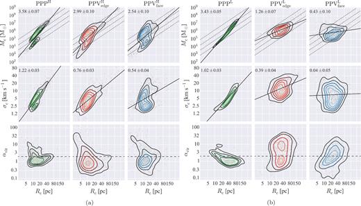
Larson's scaling relations for the identified clouds. From the top to bottom rows, relations for mass–radius (Mc–Rc), velocity dispersion–radius (σc–Rc), and virial parameter–radius (αvir–Rc) are presented, respectively. The horizontal dashed line in the αvir–Rc relation marks the boundary of virial equilibrium, where αvir = 2. The left to right columns show the results of PPP, PPVedge, and PPVface, respectively. Power-law indices of the first two relations are given in the upper-left corner of the panels. (a) Results with high resolution. Dotted lines denote Σc = 50 (lower), 230, 1000, and 5000 (upper) M⊙ pc−2, respectively. (b) Results with low resolution. It is clear that both resolution and inclination effects influence the observed GMC properties and the slopes of Larson's scaling relations.
4.3.1 Mass–radius relation
In all cases, the Mc–Rc relation shows a strong correlation. In the high-resolution clouds, the best-fitting line gives a power-law index a ≈ 3.6 for PPPH. This is a result of the bimodal Σc, for which both sequences have gradient of 3. a ≈ 3 for 3D clouds indicates that the GMCs have constant volume densities. The same index is found for the PPP clumps of Shetty et al. (2010). For PPV|$\mathrm{_{edge}^{H}}$| and PPV|$\mathrm{_{face}^{H}}$|, the best-fitting indices with all clouds are a ≈ 3.0 and 2.5, respectively.
Observations of the edge-on Milky Way normally found a value of 2.0 < a < 3.0 (e.g. Solomon et al. 1987; Simon et al. 2001; Roman-Duval et al. 2010); our value is located in the higher end. Face-on observations of nearby galaxies have not achieved such high resolution. Observations of the relatively face-on (barred) spiral galaxies Large Magellanic Cloud and M33 yielded an index a of 2.23 ± 0.08 and 1.89 ± 0.16 with an observed resolution lower than our PPV|$\mathrm{_{face}^{H}}$| data but higher than PPV|$\mathrm{_{face}^{L}}$| (Rosolowsky et al. 2003; Wong et al. 2011). The index of PPV|$\mathrm{_{face}^{H}}$| is comparable to the simulated PPV clumps of Shetty et al. (2010), where they also took a projection along the z-axis.
The discrepancy between PPV|$\mathrm{_{edge}^{H}}$| and PPV|$\mathrm{_{face}^{H}}$| originates from the different slopes of their low-Σc clouds (<230 M⊙ pc−2) that form in tidal tails and filaments, with a = 3.19 ± 0.13 for PPV|$\mathrm{_{edge}^{H}}$| and a = 2.44 ± 0.06 for PPV|$\mathrm{_{face}^{H}}$|. This is because it is more difficult to fully identify the cloud boundary of small clouds in PPV space (Shetty et al. 2010; Pan et al. 2015). Moreover, some of the low-mass PPVH clouds are part of larger PPPH clouds. PPPH cloud can be split due to internal motions or the projected density of substructures below the noise level. Finally, the steep a of the low-Σc PPV|$\mathrm{_{edge}^{H}}$| clouds is also attributed to the rapid growth in cloud mass by the blending and projection effect with respect to the confined cloud radius due to the flat disc.
For the high-Σc clouds (>230 M⊙ pc−2), PPV|$\mathrm{_{edge}^{H}}$| and PPV|$\mathrm{_{face}^{H}}$| show similar slopes, with a = 2.00 ± 0.07 and 2.15 ± 0.10, respectively, implying that structures with larger mass are more likely to have constant column densities. However, this has to be considered with caution because there are a few factors that might have caused the uniform Σc. The mass (flux) contrast between the core(s) and envelope of a PPV|$\mathrm{_{edge}^{H}}$| cloud may be reduced when the extended envelope is projected along a specific LOS that increases the observed Σc, leading to a relatively uniform Σc on the surface of the cloud. The aforementioned mass weighting causes PPV|$\mathrm{_{face}^{H}}$| cloud radii to be dominated by the high-density (mass) cores; therefore, the Mc–Rc relation is dominated by particular regions (Pan et al. 2015). This effect would be reduced to some extent in real observations since the dense regions are consumed to form stars when the density is sufficiently high. This means that the difference between a of PPV|$\mathrm{_{edge}^{H}}$| and PPV|$\mathrm{_{face}^{H}}$| would enlarge because the relation of PPV|$\mathrm{_{face}^{H}}$| would become shallower. Taking account of these, we cannot conclude that the column density of the high-Σc clouds is equivalent everywhere in these synthetic observations.
Moving to the low-resolution clouds in Fig. 5(b), power-law indices a decrease strongly when the resolution is lowered. This is true for all data structures. The power-law index of PPPL, PPV|$\mathrm{_{edge}^{L}}$|, and PPV|$\mathrm{_{face}^{L}}$| decreases to a ≈ 3.4, 1.3, and 0.6, respectively. The reason for the decreasing a is that the resolution has a notable effect on the cloud surface density, where the high-Σc population is missing due to the increase in radius, pushing their relation to low Σc for a given mass. It is worth noting that the order of the three slopes is not changed as we progress to lower resolution. In PPV|$\mathrm{_{face}^{L}}$|, there is an outlier group of relatively massive clouds sitting at mass ≥106 M⊙ but with radii of ≤20 pc. The radii of these massive non-star-forming clouds are likely underestimated due to the high-density cores taking over the weighting. These clouds occupy about 10 per cent of total populations. Even excluding these clouds arbitrarily, the Mc–Rc relation of PPV|$\mathrm{_{face}^{L}}$| is still flatter than that of PPV|$\mathrm{_{edge}^{L}}$|.
Low-resolution observations of nearby galaxies obtain an index a in the range of ∼1.5–2.6 (Engargiola et al. 2003; Bolatto et al. 2008; Rebolledo et al. 2012; Donovan Meyer et al. 2013; Colombo et al. 2014; Utomo et al. 2015). The values are larger than our derived values for both PPVH. In observations, Mc is usually calculated by adopting a constant XCO for all clouds, or represented by the measured CO luminosity (LCO). However, there is growing evidence that XCO is not constant among GMCs. Small clouds which have higher fraction of CO-dark molecular gas require larger XCO to recover the H2 mass from LCO. Thus, we would expect that the observed Mc–Rc of nearby galaxies would become shallower once the variable XCO is considered.
4.3.2 Velocity dispersion–radius relation
Results of σc–Rc are shown in the middle panels of Fig. 5. The best fits of all clouds produce a gradient of b ≈ 1.2 for PPPH and b ≈ 1.0 for PPPL. Variation of the σc–Rc relation is seen for both resolutions at low (<4 km s−1) and high (>4 km s−1) σc. We thus also perform the fit only considering those structures separately, yielding b = 0.50 ± 0.05 and 0.46 ± 0.03 for the low-σc clouds in PPPH and PPPL, and b = 1.13 ± 0.02 and 1.05 ± 0.06 for the high-σc structures, respectively. The results suggest that resolution has relatively small effect on both Larson's relations when the cloud properties are extracted from three-dimensional measurements. But note that the high- and low-σc (or Σc) clouds are relatively discrete in the high-resolution relations, while they are continuous in the low-resolution relations due to the removal of the three types of populations.
For the PPV clouds, there is a large discrepancy in the σc–Rc relation between the four data sets. As seen in the Mc–Rc relation, the best-fitting power-law indices flatten from high to low resolution, and from edge-on to face-on observation with b ≈ 0.8 and 0.5 for PPV|$\mathrm{_{edge}^{H}}$| and PPV|$\mathrm{_{face}^{H}}$| and b ≈ 0.4 and 0.0 for PPV|$\mathrm{_{edge}^{L}}$| and PPV|$\mathrm{_{face}^{L}}$|, respectively. Observations also suggest a large range of index within b ≈ 0–2, and there is no obvious correlation between the observed resolution, disc inclination, and the derived index (Engargiola et al. 2003; Rosolowsky et al. 2003; Rosolowsky 2007; Bolatto et al. 2008; Wong et al. 2011; Donovan Meyer et al. 2013; Colombo et al. 2014; Rebolledo et al. 2015; Utomo et al. 2015). Interestingly, the weak to no correlations of PPV|$\mathrm{_{edge}^{L}}$| and PPV|$\mathrm{_{face}^{L}}$| are in line with the latest unresolved observations of GMCs (Colombo et al. 2014; Leroy et al. 2015; Rebolledo et al. 2015; Utomo et al. 2015).
In fact, it is unlikely that the σc–Rc relation would be identical between PPV data sets when both variables are projection dependent but molecular clouds have non-spherical shapes (e.g. Falgarone, Phillips & Walker 1991; Shetty et al. 2010; Khoperskov et al. 2016). For example, if the LOS goes along the short dimension of the cloud, the use of PPV can result in an overestimation of Rc along with an underestimation of σc. This can explain why the high-resolution face-on observations suggest large number of clouds with low σc (Figs 2d and 5a).
A notable feature of the power-law indices a and b is the marked difference across low-resolution data sets compared to high resolution. The discrepancy arises maybe because the resolution of ∼24 pc can randomly sample various combination of cloud (or ISM) structures (see also Calzetti, Liu & Koda 2012). In other words, the resolution resolves neither the individual GMCs nor the full cloud mass spectrum, which may be used to interpret the composition of GMCs within an area. The measured cloud properties are therefore sensitive to their intrinsic properties and the geometry of cloud distribution, which includes the intrinsic and projected distributions. Hence, the derived cloud properties and the scaling relation with this resolution are not entirely driven by the underlying physical origin.
Our results of two Larson's relations suggest that such scaling relations may not genuinely reflect the physical properties and the dynamical state of GMCs. Therefore, Larson's relations should not be used alone to interpret the physical properties and the environmental dependence of GMCs.
4.3.3 Virial parameter–radius relation
PPP|$\mathrm{_{edge}^{H}}$| clouds show two populations on the αvir–Rc plane in the bottom row of Fig. 5(a). The unbound population (αvir > 2) sitting at the small-Rc regime shows decreasing αvir with Rc, i.e. the smaller clouds are the least gravitationally bound. These are the ‘Type C’ clouds with Σc < 230 M⊙ pc−2. The bound population with αvir ≈ 1 spreads out over a wide range of Rc and show αvir increasing with Rc. These are the ‘Type A’ and ‘Type B’ with high Σc.
The three cloud types and their distinct αvir are reproduced but more scattered in PPV|$\mathrm{_{edge}^{H}}$| and PPV|$\mathrm{_{face}^{H}}$| clouds (Pan et al. 2015). Overall, PPV|$\mathrm{_{face}^{H}}$| clouds share the same features as PPPH. For the PPV|$\mathrm{_{edge}^{H}}$| clouds, even though the Type C clouds are not clear in the Mc–Rc relation, it is visible in the αvir–Rc relation. This population has considerably high αvir and shows the same variation in Rc as seen in PPPH and PPV|$\mathrm{_{face}^{H}}$|. The bound population of PPV|$\mathrm{_{edge}^{H}}$|, however, shows a weak correlation between αvir and Rc. The values are concentrated around 1 from Rc ≈ 5–50 pc, but slightly increase towards Rc ≈ 80 pc. This is because Rc of PPV|$\mathrm{_{edge}^{H}}$| clouds are relatively uniform around 10 pc (Fig. 2c) due to the flat galactic disc.
Turning to the low resolution, PPPL clouds show similar features to PPPH in the αvir–Rc relation; however, the variation of cloud properties has a very notable effect on αvir for the low-resolution PPV cloud (bottom rows of Fig. 5b). αvir for PPV|$\mathrm{_{face}^{L}}$| clouds increase with Rc, indicating that the large clouds are least bound. The pattern and the underlying implication are similar to the bound population in its high-resolution counterpart, but the relation is much more scattered. We note that a high-αvir cloud is harder to detect than a lower-αvir cloud with the same Mc because the spread over larger Rc or σc will make the surface brightness per channel lower. PPV|$\mathrm{_{edge}^{L}}$| clouds show different distribution characteristics, including two concentrations with a dominant population at αvir ≈ 1 and a secondary at αvir ≈ 3–10. We found that the unbound populations tend to have relatively large σc and small Mc. Because αvir is proportional to the square of σc and inverse of Mc, αvir then increases significantly. This is in agreement with previous argument that small clouds are more susceptible to (velocity) blending. The blended emission can spread out over a wide velocity channels, but Mc does not increase as fast as σc since they are intrinsically small.
The large discrepancy in αvir can lead to inaccurate interpretations of the dynamical state of GMCs, and therefore their potential for star formation (e.g. Ballesteros-Paredes 2006). Shetty et al. (2010) and Beaumont et al. (2013) have also recognized the difficulty to determine αvir in their simulated PPV clumps even though the clumps are more compact with less substructure than our GMCs. Shetty et al. (2010) further suggest that the classic derivation of αvir for simple spherical structures may not be sufficient to reliably determine if a GMC is bound or not. Revision is required to handle the non-spherical shapes and projection effects and to include additional physics in both PPP and PPV clouds, such as Σc, magnetic fields, and time (Bertoldi & McKee 1992; Ballesteros-Paredes 2006; Dib et al. 2007; Shetty et al. 2010; Hernandez & Tan 2011). That is, dynamical state of the GMCs may not be single value to be determined.
Moreover, our results suggest that the virial mass (Mvir)-based analysis of extragalactic XCO should be used with caution. Many studies have used the classically derived Mvir (Section 3) of GMCs to estimate the extragalactic XCO assuming virial equilibrium (Mvir ≈ Mc; e.g. Adler et al. 1992; Israel et al. 2003; Rosolowsky 2007; Bolatto et al. 2008; Hughes et al. 2010; Donovan Meyer et al. 2012; Rebolledo et al. 2012). However, our results show that Mvir is projection dependent in the PPV space, and therefore the derived XCO would be affected by the observational bias as well. This is particularly true for the low, but realistic, resolution. The estimation of XCO can be improved by increasing the observed resolution as suggested by the similar αvir between the high-resolution data sets (Fig. 2f); however, the required resolution can be rather unrealistic for extragalactic observations even with ALMA, e.g. the 1.5 pc in this work.
The results for αvir also imply a significant role for the cloud definition method and selection criteria (e.g. Issa, MacLaren & Wolfendale 1990; Sheth et al. 2008; Shetty et al. 2012; Hughes et al. 2013; Fujimoto et al. 2014; Colombo et al. 2015; Pan et al. 2015). There is no obvious edge to the clouds, which are often thought to be borderline of gravitationally bound. However, the required boundary that truncates the cloud from a continuous ISM can change if the clouds are observed from a different direction, different resolution, and different data structure. We emphasize that our analysis is on the basis of a specific cloud identification method which can potentially identify the same objects with close properties between simulations and observations (Pan et al. 2015). It is not necessarily the most suitable method for other data sets, depending on the data quality and the scientific goal. The major reason for the ambiguity here is the absence of a practical ‘definition’ of a GMC.
5 SUMMARY
While ALMA is about to resolve a wide population of GMCs across different galaxy environments, understanding the observational bias is essential for obtaining reliable GMC properties. Observational bias, such as the disc inclination and the observed resolution in this work, is assessable by comparing GMC properties found when using observational identification techniques to those typically used for simulation data. To achieve this, we compared the physical properties of GMCs formed in a simulation of a barred spiral galaxy using both simulation and observational identification methods. The two methods identified clouds in the data using the PPP space typical for simulations and the PPV space used in observations. In each case, two resolutions were considered: one at the maximum resolution of the simulation data (1.5 pc) and another at a more realistic level for observational instruments (24 pc). For the PPV data, the galaxy disc was also considered both face-on and side-on, to explore the result of projection effects. The PPV data cube was assumed to be the product of 12CO (1–0) observations.
The main results for the high-resolution (1.5 pc) cloud properties in PPPH, PPV|$\mathrm{^{H}_{edge}}$|, and PPV|$\mathrm{^{H}_{face}}$| are as follows.
The galactocentric profiles of cloud numbers are similar in all data sets, showing two concentrations at the radii of galactic bar and spiral arms. However, the cloud number in the PPV|$\mathrm{^{H}_{edge}}$| analysis lies below the PPPH and PPV|$\mathrm{^{H}_{face}}$| data sets by roughly a factor of 2, indicating that the clouds are blending when viewed edge-on in PPV space. Thus, even though the distribution and median values of the high-resolution cloud properties (mass and velocity dispersion) agree with each other, this should not lead to the interpretation that the clouds in PPV|$\mathrm{^{H}_{edge}}$| and PPPH/PPV|$\mathrm{^{H}_{face}}$| are completely the same.
Disc inclination has a notable effect on the cloud radius where the results from the PPV|$\mathrm{^{H}_{edge}}$| become smaller than the other two data sets due to the flat galactic disc.
The bimodal mass surface density distribution of PPPH clouds as a result of different formation mechanisms suggested in Fujimoto et al. (2014) is reproduced by both the PPV|$\mathrm{^{H}_{edge}}$| and PPV|$\mathrm{^{H}_{face}}$| methods, although the boundary between the two trends is least distinguishable for PPV|$\mathrm{^{H}_{edge}}$|, due to small populations being particularly susceptible to blending.
The data structure and disc inclination do not significantly affect the virial parameter of the high-resolution clouds. All methods determined a median virial parameter of ∼1.0, suggesting that majority of clouds are gravitationally bound.
We prepared low-resolution (24 pc) PPV data sets using casa, allowing us to simulate ALMA observation with realistic resolution and sensitivity (noise level). The low-resolution PPP clouds were identified from a simulation with fewer total levels of refinement. The main results for the low-resolution cloud properties in the PPPL, PPV|$\mathrm{^{L}_{edge}}$|, and PPV|$\mathrm{^{L}_{face}}$| data sets are as follows.
We first compared the results from PPPL and PPPH to evaluate the blending (or resolution) effect alone. This revealed that although the cloud properties change, the simulation can potentially see the spatial distribution and dynamical state of clouds regardless of resolution. However, it is not able to distinguish clouds formed via different formation mechanisms at 24 pc resolution, even though the cloud properties are extracted directly from three dimensions.
When we switched from high to low resolution (and sensitivity) in observations, the smaller clouds are lost. Large clouds are detected but become more spherical than their intrinsic morphology due to the image convolution with the nearly circular beam.
The galactocentric profile of PPV|$\mathrm{^{L}_{edge}}$| no longer represents the intrinsic distribution of clouds, but declines with radius, whereas PPV|$\mathrm{^{L}_{face}}$| show a similar profile as PPPL and their high-resolution counterparts, but with fewer clouds at all radii.
Overall, we found good agreement between the profiles and median values of the cloud properties between the PPV|$\mathrm{^{L}_{face}}$| and PPPL techniques, while PPV|$\mathrm{^{L}_{edge}}$| clouds are more massive and with larger velocity dispersions.
In contrast with the high-resolution data, the mass density is not bimodal in any of the low-resolution data.
The resolution has an alarming effect on the virial parameter. Median αvir of PPV|$\mathrm{^{L}_{edge}}$| suggests that the clouds are not gravitationally bound, which is in contrast to PPPL and PPV|$\mathrm{^{L}_{face}}$|, where the clouds seem to be bound.
We plotted Larson's scaling relations of mass–radius (Mc ∝ Rca) and velocity dispersion–radius (σc ∝ Rcb) using the measured cloud properties; the main results are as follows.
The power-law indices of the Larson relations change with data structure, disc inclination, and resolution. In all relations, the indices decrease from PPP, PPVedge to PPVface and decrease from high to low resolutions.
For individual data structures, the power-law index of PPP is relatively insensitive to resolution, while it changes by ≥2 times between the two resolutions for both face-on and edge-on PPV. This suggests that Larson's scaling might be reliable only for the cloud properties extracted from three dimensions.
A discrepancy in the power-law indices between face-on and edge-on observations is also observed. Moreover, the low, but realistic, resolution shows larger discrepancy compared to high resolution. Perhaps because a 24 pc resolution can sample clouds with various combinations, the measured cloud properties and the scaling relations are therefore not representing the true cloud properties.
We also compared the relation between the virial parameter (αvir) and Rc. Results suggest that such scaling relations are not entirely driven by the underlying physical origin of the GMCs. Therefore, they should be used with caution when discussing the environmental dependence and the dynamical state of GMCs.
We made a few comments on the CO-to-H2 conversion factor (XCO) in real observations. First of all, the differences in the cloud mass between the low-resolution data sets are comparable to the uncertainty of XCO. Thus, the observational bias can be obscured by adopting a different XCO. Secondly, that a virial mass-based derivation of extragalactic XCO should be used with caution. Our results show that Mvir is projection dependent in the PPV space, especially with the low but realistic resolution (24 pc). Therefore, the derived XCO would be affected by the observational bias as well. The estimation of XCO can be improved by increasing the observed resolution. However, the required resolution can be rather unrealistic for extragalactic observations even with ALMA, e.g. the 1.5 pc in this work.
Finally, we note that this work is based on a specific setup for a simulated galaxy. Observational bias would alter the GMC properties and Larson's relations in different ways if the galaxy type is changed, such as the global morphology and gas content, because they determine the intrinsic distribution and properties of the GMCs.
We thank referee for providing useful comments that have helped to improve the paper. We would like to thank the yt development team (Turk et al. 2011) for support during the analysis of these simulations. Numerical computations were carried out on the Cray XT4 and Cray XC30 at the Center for Computational Astrophysics (CfCA) of the National Astronomical Observatory of Japan (NAOJ). EJT is funded by the MEXT grant for the Tenure Track System. SMB acknowledges financial support from the Vanier Canada Graduate Scholarship programme.
REFERENCES
