


Abstract
We present six epochs of spectropolarimetric observations and one epoch of spectroscopy of the Type Ib SN iPTF 13bvn. The epochs of these observations correspond to −10 to +61 d with respect to the r-band light-curve maximum. The continuum is intrinsically polarized to the 0.2–0.4 per cent level throughout the observations, implying asphericities of ∼10 per cent in the shape of the photosphere. We observe significant line polarization associated with the spectral features of Ca ii ir3, He i/Na i d, He i λλ6678, 7065, Fe ii λ4924 and O i λ7774. We propose that an absorption feature at ∼6200 Å, usually identified as Si ii λ6355, is most likely to be high-velocity H α at −16 400 km s−1. Two distinctly polarized components, separated in velocity, are detected for both He i/Na i d and Ca ii ir3 , indicating the presence of two discrete line-forming regions in the ejecta in both radial velocity space and in the plane of the sky. We use the polarization of He i λ5876 as a tracer of sources of non-thermal excitation in the ejecta; finding that the bulk of the radioactive nickel was constrained to lie interior to ∼50–65 per cent of the ejecta radius. The observed polarization is also discussed in the context of the possible progenitor system of iPTF 13bvn, with our observations favouring the explosion of a star with an extended, distorted envelope rather than a compact Wolf–Rayet star.
1 INTRODUCTION
The most intriguing and mysterious aspect of the cataclysmic death of massive stars as supernovae (SNe) is the explosion mechanism itself. The driving force of the explosion is the subject of numerous theoretical models (see recent reviews in Burrows 2013 and Janka 2012), where the distinguishing feature between the models is the resulting geometry of the explosion. The vast majority of extragalactic SNe, however, are too distant for their geometries to be directly spatially resolved with currently available, or even planned, telescope facilities. Spectropolarimetry is a powerful probe of the 3D geometries of unresolved SNe and can therefore aid in pinning down the nature of the explosion.
Previous polarimetric studies have shown that departures from spherical symmetry are present in most if not all SNe (Wang & Wheeler 2008). Thermonuclear Type Ia SN explosions exhibit strong polarization associated with absorption lines before peak luminosity, which subsequently decrease in strength as the SNe evolve. This implies that the inner ejecta are more spherical than the outer layers. Conversely, core-collapse SNe (CCSNe) such as SNe 1993J, 2002ap, 2005bf and 2008D were observed to be highly polarized across particular lines and show asymmetries in the shape of the photosphere of the order of ∼10 per cent (Trammell, Hines & Wheeler 1993; Tran et al. 1997; Kawabata et al. 2002; Wang et al. 2003; Maund et al. 2007a, 2009). In CCSNe, the degree of asymmetry appears to increase as the photosphere recedes into the deeper layers of the ejecta. The Type IIP SN 2004dj showed a dramatic increase in the continuum polarization as the photosphere receded through the hydrogen layer into the core, unambiguously signalling that the explosion mechanism itself was inherently asymmetric and previously shielded from view by the hydrogen envelope at earlier times (Leonard et al. 2006). Polarimetry of SNe arising from progenitors that have been stripped of their outer hydrogen envelope probes the geometry of the explosion at early times.
iPTF 13bvn was discovered by the Intermediate Palomar Transient Factory (iPTF; Law et al. 2009) on 2013 June 16.238 in galaxy NGC 5806 (22.5 Mpc) and was classified as a Type Ib SN. According to Cao et al. (2013), the SN was discovered very early at only 0.57 d after their estimated explosion date of 2013 June 15.67. The SN reached a peak maximum brightness of Mr = −16.6 on 2013 July 3 (18 d later).
iPTF 13bvn is the first Type Ib SN for which a possible progenitor candidate has been detected; however, the nature of the progenitor candidate is unclear. Cao et al. (2013) identified a blue object in Hubble Space Telescope/Advanced Camera for Surveys pre-explosion observations, consistent with a single Wolf–Rayet (WR) star. This conclusion was supported by Groh, Georgy & Ekström (2013) who constrained the initial mass to 31–35 M⊙(∼11 M⊙ pre-SN), and predicted a large ejecta mass (∼8 M⊙). Fremling et al. (2014) and Srivastav, Anupama & Sahu (2014) both constrained the ejected mass to ∼2 M⊙, which is inconsistent with the explosion of such a massive WR star. Furthermore, hydrodynamical models of Bersten et al. (2014) suggested that the progenitor had a mass of 3.5 M⊙ prior to the explosion and proposed an interacting binary as the progenitor channel. Reanalysis of the pre-explosion photometry and comparison with binary evolution models by Eldridge et al. (2015) also suggested that the progenitor was likely to be a low-mass helium giant star (initial mass 10–20 M⊙) in an interacting binary system.
Spectroscopically, iPTF 13bvn showed similarities to Type Ib SNe 2009jf, 2008D and 2007Y (Fremling et al. 2014; Srivastav et al. 2014). The light curve, however, showed a much faster decline than most Type Ib/c SNe and a lower peak brightness luminosity (Srivastav et al. 2014). Reproduction of the light curve with hydrodynamical models required 0.05–0.1 M⊙ of nickel (consistent with an estimate by Srivastav et al. 2014) to be highly mixed out to the outermost layers of the ejecta to reproduce the rise time (Fremling et al. 2014; Bersten et al. 2014, but note that there may be issues with the treatment of opacity in standard models of the peaks of stripped-envelope SNe (Wheeler, Johnson & Clocchiatti 2015).
Here, we present multi-epoch spectropolarimetry of iPTF 13bvn acquired with the European Southern Observatory (ESO) Very Large Telescope (VLT), covering from −10 to +36 d with respect to the r-band peak luminosity plus an additional epoch of spectroscopy at +61 d. The sections are organized as follows: the observations and data reduction are presented in Section 2; the results of the observations are presented and analysed in Sections 3 and 4, respectively. In Section 5, the results and analysis are discussed and in Section 6 we present our conclusions.
2 OBSERVATIONS AND DATA REDUCTION
Observations of iPTF 13bvn were acquired using the ESO VLT Antu (Unit 1) telescope and the Focal Reducer and Low Dispersion Spectrograph (FORS2) instrument in the spectropolarimetric PMOS and long-slit LSS modes (Appenzeller et al. 1998). Six epochs of spectropolarimetric data and one epoch of spectroscopic data were obtained. A log of the observations can be found in Table 1. For the polarimetric observations, the half-wavelength retarder plate was positioned at four angles (0, 22|$_{.}^{\circ}$|5, 45°, 67|$_{.}^{\circ}$|5) through two iterations, resulting in eight exposures at each epoch. Observations were acquired with the 300 V grism, which provides a spectral resolution of 12 Å as measured from arc lamp calibration frames. The GG435 order separation filter was used to prevent second-order contamination at longer wavelengths, resulting in a final wavelength range of 4450–8650 Å. The data were reduced in the standard manner using iraf,1 following the prescription of Maund et al. (2007a), and the normalized Stokes parameters (q and u) were calculated following Patat & Romaniello (2006). The data were corrected for the wavelength dependent chromatic zero-angle offset of the retarder plate, and the polarization spectra were further corrected for bias following Quinn et al. (2012). In order to increase the signal-to-noise level, the data were rebinned to 15 Å, prior to the calculation of the Stokes parameters. Flux spectra of the SN at each epoch of polarimetry were calibrated using observations of a flux standard star with the polarimetry optics in place and the retarder plate at 0°. The flux spectrum at +61 d was calibrated in the standard manner using observations of the flux standard LTT 7379.
Table of VLT FORS2 observations of iPTF 13bvn.
| Object | Date | Exposure | Mean | Epocha | S/Nd |
|---|---|---|---|---|---|
| (ut) | (s) | airmass | (d) | ||
| iPTF 13bvn | 2013 06 23 | 8 × 870 | 1.16 | −10 | 410 |
| LTT 6248b | 2013 06 23 | 40 | 1.00 | ||
| iPTF 13bvn | 2013 07 04 | 8 × 855 | 1.13 | 0 | 740 |
| LTT 6248b | 2013 07 04 | 80 | 1.02 | ||
| iPTF 13bvn | 2013 07 10 | 8 × 855 | 1.43 | +7 | 640 |
| LTT 6248b | 2013 07 10 | 45 | 1.40 | ||
| iPTF 13bvn | 2013 07 12 | 8 × 855 | 1.37 | +9 | 660 |
| LTT 6248b | 2013 07 12 | 45 | 1.01 | ||
| iPTF 13bvn | 2013 07 28 | 8 × 855 | 1.32 | +25 | 350 |
| LTT 6248b | 2013 07 28 | 90 | 1.1 | ||
| iPTF 13bvn | 2013 08 08 | 8 × 855 | 1.68 | +36 | 270 |
| LTT 6248b | 2013 08 08 | 90 | 1.05 | ||
| iPTF 13bvnc | 2013 09 02 | 3 × 1180 | 1.79 | +61 | |
| LTT 7379cb | 2013 09 02 | 3 | 1.08 |
3 SPECTRAL EVOLUTION
The flux spectra and degree of polarization, p, of iPTF 13bvn for the six epochs of spectropolarimetric observations and one epoch of late-time spectroscopy are presented in Fig. 1. The phases indicated are with respect to the r-band maximum on 2013 July 3 (Cao et al. 2013).
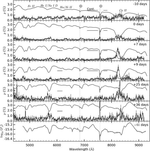
The polarization spectra of iPTF 13bvn from −10 d to +36 d relative to the r-band maximum. At each epoch, the flux spectra (log10(Fλ)) are shown by the thick grey lines and are corrected for the recessional velocity of the host galaxy (1359 km s−1, as quoted by NED). The flux spectrum from the spectroscopic observations at +61 d is also shown in the bottom panel. The horizontal bars indicate the wavelength regions used to measure the continuum polarization.
At all epochs, the flux spectra exhibit broad P Cygni profiles of Ca ii, He i and Fe ii. The flux spectra are dominated by a strong absorption due to the Ca ii near-infrared triplet (hereafter Ca ii ir3). At −10 d, the absorption exhibits a flat bottom, with a minimum at −13 300 km s−1, which steadily decreases to −7450 km s−1 at +36 d. At +7 d the absorption becomes asymmetric, appearing to be double dipped with apparent minima at −10 200 and −7000 km s−1 , with a blue edge extending to −24 000 km s−1. By +25 d, the two minima occur at −4560 and −8400 km s−1. From +25 d another absorption features appears at ∼8125 Å , corresponding to −16 200 km s−1 with respect to the weighted average rest wavelength of Ca ii ir3. Alternatively, this feature may be associated with a possible emission bump observed at 8169 Å. By +61 d, Ca iiir3 is observed to be predominantly in emission, with some evidence that the constituent lines are partially resolved. The final velocity at the absorption minimum corresponds to either −7700 km s−1 (assuming the weighted average rest wavelength for the triplet) or −5200 km s−1 (assuming the lowest rest wavelength of the individual Ca iiir3 lines 8498 Å).
Following the Ca ii ir3, the next strongest feature in the spectra is the blend of He i λ5876 and Na i d at ∼5500–5800 Å. Over the evolution of the SN, the strength of this absorption feature increases while the velocity at the absorption minimum exhibits a slower decline compared to that observed for Ca ii. The velocity (assuming a rest wavelength of 5876 Å) decreases from −11 500 km s−1 at −10 d to −8800 km s−1 at 0 d, where it appears to plateau before settling at −7900 km s−1 at +61 d. The decay in the velocity at absorption minimum for He i/Na i d , along with Ca ii ir3 and Fe ii λ5169, is plotted in Fig. 2. The He i/Na i d line profile appears asymmetric at early times with a blue edge extending up to ∼−20 000 km s−1, and, at later epochs, there is a possible higher velocity component at ∼−14 000 km s−1. He i λλ6678, 7065 are also present in the spectra, however obtaining the velocity at absorption minimum for these lines is complicated by blending with a telluric feature for He i λ7065 and with the emission component of the Si ii λ6355 P Cygni profile for He i λ6678. At +25 and +36 d, the depth of the He i λ7065 absorption component is greater than that of the telluric lines, such that the velocity at minimum absorption could be measured to be −6700 and −6500 km s−1 at +25 and +36 d, respectively.
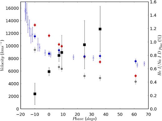
The evolution of the velocity at absorption minimum for Ca ii ir3 (red), the He i/Na i d blend (blue) and Fe ii λ5169 (a proxy for the photospheric velocity; grey). These data are marked by circles while measurements for He i/Na i d and Fe ii λ5169 from Fremling et al. (2014) are also shown here by crosses. The evolution of peak line polarization associated with the He i/Na i d blend is marked by black squares.
The absorption feature at ∼6200 Å, observed at −10 d, is frequently associated with Si ii λ6355. The strength of the line and the velocity of the absorption minimum decreases with time, eventually disappearing at +25 d. The corresponding velocity at absorption minimum of −7400 km s−1, however, is lower than the photospheric velocity at the same epoch (see below and Fig. 2). Alternatively, Parrent et al. (2015) suggest that features such as this in other Type I CCSNe may be high-velocity (HV) H α. If this feature arises instead from hydrogen the corresponding velocity at absorption at −10 d was 16 700 km s−1.
At −10 d, Fe ii is observed as an unresolved blend of doublets 38 and 42 covering the wavelength region 4800–5400 Å, before the individual lines become resolved by 0 d. Following Fremling et al. (2014), the velocity at the absorption minimum of Fe ii λ5169 is used to indicate the photospheric velocity, for which we measure a velocity of −8750 km s−1 at 0 d. The photospheric velocity steadily decreased to −4300 km s−1 by +61 d.
O i λ7774 appears as a weak P Cygni profile from +25 d onwards, having been absent at earlier epochs.
4 ANALYSIS OF THE POLARIMETRY
4.1 Interstellar polarization
Scattering of photons due to intervening dust in the interstellar medium introduces an additional component to the observed polarization. The removal of the interstellar polarization (ISP) is a vital step in correctly interpreting the intrinsic polarization of the SN. The correct determination of the ISP is non-trivial and dependent upon the assumption that certain wavelength regions of the SN spectrum are intrinsically unpolarized. One approach is to assume that resonance scattering photons are intrinsically unpolarized (Trammell et al. 1993), such as those found in strong emission lines and areas of line blanketing. Under the assumption that certain regions of the SN spectrum at certain epochs are intrinsically unpolarized and, therefore, representative of the effect of the ISP, we derive three estimates of the ISP:
ISPA. The observed polarization for intrinsically unpolarized strong resonant scattering emission lines should tend towards the ISP (as the line strength increases). The strongest emission line in the SN spectra is the Ca ii ir3 at +36 d. The Stokes parameters were averaged over a 60 Å range, redward of the emission peak, avoiding the polarization associated with the blueward absorption trough. For our first estimate of the ISP, we measured values of the polarization across this wavelength range of |$q_{{\rm ISP}_{\rm A}}$| = −0.28 ± 0.24 per cent and |$u_{{\rm ISP}_{\rm A}}$| = 0.12 ± 0.25 per cent.
ISPB. At −10 d the Fe ii 38 and 42 doublets are unresolved in the spectrum leading to a region of line blanketing which is assumed to be intrinsically unpolarized. Taking the weighted average of Stokes q and u in the wavelength region 5000–5400 Å, we derive an estimate for ISPB of |$q_{{\rm ISP}_{\rm B}}$| = −0.12 ± 0.12 per cent and |$u_{{\rm ISP}_{\rm B}}$| = 0.39 ± 0.14 per cent.
ISPC. A further estimate of the ISP was determined by averaging the polarization of the Ca ii ir3 emission line and strong emission from a possible Fe ii and He i blend (at ∼5010 Å) at +25 d. At this epoch, the spectrum appears depolarized in these regions, from which we derive ISPC as |$q_{{\rm ISP}_{\rm C}}$| = −0.19 ± 0.04 per cent and |$u_{{\rm ISP}_{\rm C}}$| = −0.10 ± 0.08 per cent.
The inverse error weighted average of the three estimates was taken as the principal estimate of the ISP, with the standard deviation as the corresponding uncertainty, resulting in qISP = −0.19 ± 0.08 per cent and uISP = 0.03 ± 0.28 per cent. The position of the principal and individual estimates of the ISP are shown on the Stokes q–u plane on Fig. 3.
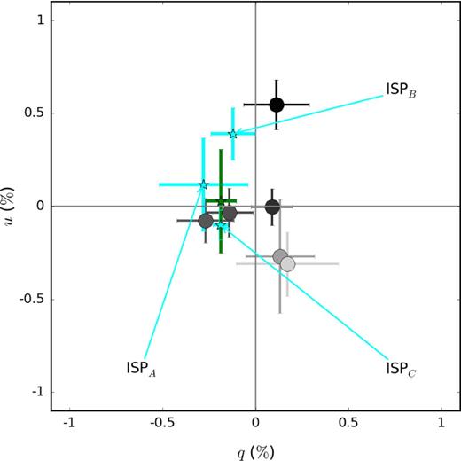
The temporal evolution of the observed continuum polarization, coloured according to phase from dark (−10 d) to light grey (+36 d). The three individual estimates of the ISP (see Section 4.1) are marked by cyan stars and the position of the average ISP estimate is marked by the green star.
The total reddening due to Galactic and host dust is E(B − V)MW = 0.0278 (Schlafly & Finkbeiner 2011) and E(B − V)host = 0.0437 (Cao et al. 2013). Assuming a Serkowski law and Galactic-type dust, this limits the degree of polarization arising from the intervening dust to be pISP ≤ 9( E(B − V)MW + E(B − V)host) = 0.64 per cent. The value we have determined for pISP = |$0.25^{+0.22 }_{ -0.17}\hbox{ per cent}$| is therefore consistent with the maximum expected given the reddening towards iPTF 13bvn.
4.2 Intrinsic continuum polarization
The level of intrinsic continuum polarization reveals the degree of asphericity in the SN photosphere. We identified regions of the spectrum of iPTF 13bvn at each epoch that were deemed to be flat in polarization and far from any lines that might contaminate the polarization (indicated by the black horizontal bars in Fig. 1). As the spectrum of iPTF 13bvn evolved, with lines appearing and disappearing, the wavelength regions we considered to be representative of the continuum also changed. The continuum polarization was measured by taking the inverse-error weighted-average of the Stokes parameters, after correction for the ISP, over the continuum wavelength ranges. The corresponding uncertainties were calculated as the standard deviation of the polarization over the continuum wavelengths ranges, with respect to the weighted mean continuum polarization. The evolution of the continuum polarization (before correction for the ISP) is shown in Fig. 3.
We find the continuum to be intrinsically polarized at the 0.2–0.4 per cent level throughout the series of observations. Due to the low level of polarization, and the relatively large uncertainties (∼± 0.13 per cent), there is little evidence for evolution in the degree of the continuum polarization to the 3σ level. The continuum polarization angle undergoes a clockwise rotation from 29 ± 9° to 177 ± 3° between the first two observations. After the second epoch, the polarization angle remains approximately constant throughout the remaining observations of +7, +25, +36 d at ∼153°; however, at +9 d, the continuum polarization angle is 117 ± 4°, despite no change in the degree of polarization, at the 0.01 per cent level, from two days before.
The inferred values for the continuum polarization are, however, sensitive to the choice of the ISP. For example, correction for ISPA yields similar values for the continuum polarization as presented above, however the continuum polarization angle at +9 d (137 ± 3°) is no longer discrepant from the angle measured immediately before. Upon subtraction of ISPB, the continuum polarization exhibits a steady increase from 0.19 ± 0.10 per cent before peak brightness to 0.59 ± 0.25 per cent at +36 d. The removal of ISPC results in the degree of continuum polarization reaching a maximum of ∼0.7 per cent at −10 d, before decreasing to 0.13 per cent at +7 d and then increasing again to 0.34 per cent at +25 d. In addition, for ISPC, the continuum polarization angle also exhibits very dynamic behaviour changing from 32 ± 6° at −10 d, to 9 ± 13° at 0 d and then 157 ± 20° at +36 d.
The maximum intrinsic continuum polarization of 0.39 per cent, after subtraction of the averaged ISP, implies asphericities of 10 per cent in the shape of the photosphere (Höflich 1991). For ISPB, the maximum continuum polarization of 0.7 per cent implies asphericities of 10–15 per cent. Although the different ISPs result in different continuum polarizations, the corresponding differences in the inferred shape of the photosphere are relatively small for iPTF 13bvn. The evolution in the alignment of the photosphere on the plane of the sky, however, is shown to be dependent on the chosen ISP. Provided that the ISP is not substantially underestimated in Section 4.1 the rotation of the continuum polarization is intrinsic to the SN.
4.3 Intrinsic line polarization
The polarization spectra, shown in Fig. 1, exhibit peaks associated with the various spectral lines identified in Section 3. In the following section, we analyse the temporal evolution of the line polarization intrinsic to iPTF 13bvn. The subsections are organized according to species and ordered from the most strongly polarized species (Ca ii) to the least (O i λ7774). The intrinsic polarization due to line absorption features was determined with the vector subtraction of the measured continuum polarization from the observed data. The observed continuum polarization is the summation of the intrinsic continuum polarization of the SN and the ISP and the subtraction of the observed continuum polarization results, therefore, in an intrinsic line polarization that is independent of the choice of the ISP.
4.3.1 Ca ii ir3
At all epochs, the polarization spectra are dominated by strong line polarization associated with the Ca ii ir3. The polarization signal evolves from a broad feature (full width at half-maximum ∼9500 km s−1 ) with degree of polarization p = 0.7 ± 0.5 per cent at −10 d to a narrower, stronger signal of p ∼2.5 per cent at +7 d. The polarization increases again to p = 3.3 ± 0.8 per cent at +25 d, with significant signal spread across a larger velocity range than was observed previously. The velocity at which the polarization across the Ca ii ir3 profiles appears to peak also increases from −9500 km s−1 at −10 d to −12 300 km s−1 at +7 d before decreasing again to −8400 km s−1 at the final epoch of spectropolarimetry. The polarization angle (at the polarization maximum) of Ca ii is similar at −10 and 0 d, with θline ∼ 70°. It then rotates to ∼120° at +7 d, where it remains throughout the rest of the observations.
There is significant structure associated with this line on the Stokes q–u plane, shown in Fig. 4. At 0 d, there is a loop that crosses all quadrants of the q–u plane, with three separate components at ∼−8000, −12 000 and −15 000 km s−1, suggesting a complex line forming structure in the plane of the sky. The shape of the loop changes at +7 d, resulting in an extended loop for velocities between ∼−7000 and ∼−15 000 km s−1, while at lower velocities the signal appears to cluster near the origin of the q–u plane and at higher velocities (≲−15 000 km s−1) the data are clustered at ∼135°. At +9 and +25 d, the feature on the q–u plane is similar to that observed +7 d, although with a higher degree of polarization p ∼3.3 per cent seen at +25 d. There is evidence of significant polarization at +36 d, however the signal-to-noise ratio is insufficient to properly discern any structure in the q–u plane at this epoch.
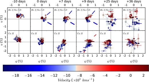
The observed polarization of the He i/Na i d blend (top panel) and Ca ii ir3 (bottom panel) on the Stokes q–u plane. The points are coloured coded according to their velocity with respect to the rest wavelength. Radial lines indicate the principal polarization angles for the LV (narrow lines) and HV (thick lines) components, for epochs at which they appear as separate features. Note the difference in scale between the top and bottom panels.

Fits to the observed degree of polarization for the Ca ii ir3 at +9 d with pline as a variable. No one value of pline can provide a complete fit to the observed polarization across the entire line profile. The best fits to LV, HV and V-HV components of the line are marked in red, blue and purple, respectively.
The behaviour of the polarization angle across the line profile displays an intriguing evolution. At −10 d, the polarization remains constant as a function of velocity at ∼70°. By maximum light, however, we observe a steady rotation in the polarization angle from ∼50° to 150° with increasing velocity. At +7 d, the polarization angle across the line profile begins to split into two separate components, with the separation between the two becoming clearly apparent by +9 d. At +9 d there is a defined break in the polarization angle at −8100 km s−1 between the two components (see Fig. 6). The LV component, at θline = 21°, is separated by ∼75° (or −55°) from the HV component (from −8100 to ∼−15 000 km s−1) at θline = 125°. At +25 d, the polarization angle changes steadily from approximately 50° at low velocities to 120° at −10 000 km s−1. The data are noisier at +36 d, however the trend in the polarization angle appears to be similar to that observed at the previous epoch.
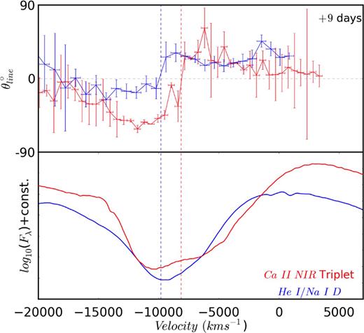
The polarization angle as a function of velocity for the Ca ii ir3 (red) and He i/Na i d (blue) profiles at +9 d. The bottom panel shows the total flux spectra across each of these profiles. The dashed lines represent the velocity of the transition between the LV and HV components for Ca ii ir3 (red, −8100 km s−1) and He i/Na i d (blue, −9800 km s−1).
While separate HV and LV components are observed for Ca ii in the polarized flux spectrum (at +9 d), an analysis of the Ca ii ir3 line profile in the flux spectrum, following the prescription of Silverman et al. (2015), was not able to recover the two separate components. The asymmetric line profile observed in the flux spectrum, from +7 d onwards, was found to result from a superposition of the individual components of the triplet (at ∼−8800 km s−1) becoming partially resolved. We note, however, that this analysis assumes that the underlying line profiles are well described by Gaussian profiles.
The fits also indicated that an additional narrow absorption feature at +25 d, at ∼8150 Å or −14 000 km s−1relative to the Ca ii ir3 rest wavelength, is probably unrelated to Ca and is probably due to another element. Although not observed at earlier epochs, the velocity of this feature places it in the ‘blue wing’ or V-HV component of the Ca ii ir3 absorption. This could suggest that the extreme line polarization measured for the V-HV component at +9 d may not actually be due to Ca. Conversely, we note that if this separate species were responsible for the polarization of V-HV component, the degree of polarization would appear to be anticorrelated with the increasing strength of the line in the flux spectrum at later epochs. The presence of two components in the He i/Na i d profiles (discussed in Section 4.3.2) leads us to conclude that the separate LV and HV components Ca ii are real.
4.3.2 He i λλ5876, 6678, 7065 and Na i D
Polarization is also associated with the He i absorption lines, most prominently seen in the He i/Na i d blend. The intrinsic degree of polarization of the He i/Na i d blend grows from pline = 0.29 ± 0.06 per cent at −10 d to 1.2 ± 0.3 per cent at the final epoch of polarimetry. At −10 d, the data points of the He i/Na i d blend cluster around the position of the continuum polarization on the Stokes q–u plane (see Fig. 4). By 0 d, the points begin to separate into two polarized clusters, at ∼20° and ∼165° for velocities ≳−8000 and ≲−8000 km s−1, respectively.
At earlier epochs, the polarization peak occurs redward of the absorption minimum, at a velocity of −6200 km s−1 between −10 and +7 d. The velocity at which the polarization maximum occurs dramatically increases at later times to −11 900 and −10 200 km s−1 at +25 and +36 d, respectively. The significant increase in the velocity of the maximum degree of polarization is accompanied by a rotation in the polarization angle from θline = 20 ± 8° at +9 d to θline = 128 ± 9° at +25 d. The increase in velocity and the rotation of the polarization angle at +25 d appears to be the result of an HV component becoming more strongly polarized than the LV component (that dominated the polarization at earlier epochs) as can be seen on Figs 1 and 4.
As was observed for Ca ii, the polarization angle for He i/Na i d blend also exhibits a discontinuity at +7 and +9 d (see Fig. 6). This discontinuity occurs at −9800 km s−1, which is higher than the velocity of the discontinuity observed for Ca ii. For He i/Na i d, the LV component has a polarization angle of θline = 25° and is separated by 40° from the HV component at θline = 165° (or −15°). At +25 d, the polarization angle is constant at ∼47° for velocities less than −6500 km s−1, before increasing to 141° at −14 000 km s−1. A similar trend is observed at +36 d.
For He i λ6678 , significant polarization is only observed at the final epoch; with pline = 1.0 ± 0.3 per cent and θline = 180 ± 9°. Conversely, polarization is observed for He i λ7065 at 0, +9 and +36 d. The degree of polarization of He i λ7065 reaches a maximum at +9 d with pline = 0.73 ± 0.06 per cent and θline = 10 ± 2°, before undergoing a rotation in the polarization angle to 138 ± 14° at +36 d. The lack of significant polarization across the He i λ7065 and He i λ6678 lines at all epochs makes it difficult to determine to what degree the Na i doublet contributes to the polarization of the He i/Na i d blend. The shape of the He i λ5876 and He i λ7065 line profiles show good agreement at 0, +7 and +9 d, which may indicate a minimal contribution from Na at these epochs. At −10, +25 and +36 d, however, the line profiles are different, with the velocity at the He i λ5876 absorption minimum being substantially higher. The agreement between the He i/Na i d and He i λ7065 polarization angles at low velocities (≳−4000 km s−1) suggests He dominates the polarization signal in that velocity range.
We conclude that the HV He i component, although weakly polarized and potentially contaminated by the polarized Na i doublet, is a real feature and represents a separate line-forming region for He i at high velocities. Contamination from polarized Na i d would result in a steady rotation of the polarization angle, rather than the discontinuity observed in Fig. 6.
4.3.3 Fe ii
Peaks in the polarization are also observed around 4700–4800 Å, coincident with an Fe ii absorption trough. As such, we associate it with the nearest redward strong emission of Fe ii λ4924. The strength of the polarization grows from p = 0.54 ± 0.26 per cent at −10 d to p = 1.4 ± 1.0 per cent at +36 d. The uncertainty on the last measurement is large and the feature appears to be due to one elevated bin at −5000 km s−1(which may indicate that the feature at +36 d is an artefact from the reduction). The Fe ii λ4924 feature is polarized to the ∼0.6 per cent level for the majority of the observations. The velocity of the maximum polarization initially increases from −9800 to −13 800 km s−1 between −10 and 0 d, before decreasing back to −9800 km s−1 at +9 d and then increasing again to −11 800 km s−1 at +25 d. The polarization angle rotates from θline = 83 ± 14° in the first epoch to ∼135° at 0 d; it then remains approximately constant throughout the remainder of the observations.
Given the significant polarization associated with Fe ii λ4924 at −10 d, it is likely that the 5000–5400 Å wavelength region, used to estimate ISPB, is contaminated with polarization associated with the absorption troughs of the overlapping Fe ii lines in the region. Therefore, it is possible that ISPB is a poor estimate of the interstellar polarization. Upon removal of ISPB from consideration, the inverse error weighted average of the ISP remains unchanged within the quoted uncertainties.
4.3.4 The 6200 Å feature
Significant polarization is associated with the absorption at ∼6200 Å in the first two epochs, with a maximum polarization of p = 0.59 ± 0.06 per cent at −10 d. If this feature is due to Si ii, the velocity of the polarized feature decreases from −6400 to −3500 km s−1 between −10 and 0 d. Alternatively, if the feature is H α then the velocities at the two epochs are, instead, −16 400 to −13 400 km s−1. Between −10 and 0 d, there is also a small rotation in the polarization angle from θline = 76 ± 3° to θline = 63 ± 7°. Significant polarization is not observed after 0 d, when the strength of the absorption feature decreases until it disappears by +25 d.
4.3.5 O i
O i λ7774 appears in the spectrum as a weak P Cygni profile from +25 d onwards. Upon removal of the continuum polarization O i remains significantly polarized at +36 d. We estimate a polarization associated with O i of 0.66 ± 0.13 per cent at −3800 km s−1 at +36 d, with θline = 154 ± 6°; however, this measurement is complicated by the proximity of the line to a telluric feature.
4.4 The polarimetric evolution in the plane of the sky
The measured polarization angles provide an indication of the locations of the line-forming regions for different species in the plane of the sky. Maund et al. (2009) suggested a new type of polar plot for spectropolarimetric data that may be used to illustrate the relative positions of the different line-forming regions in radial velocity space and in the plane of the sky. These polar plots, or Maund diagrams, provide a projection of the approximate 3D structure of the SN ejecta independently of models. The spectropolarimetric observations of iPTF 13bvn are presented in this form on Fig. 7.
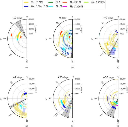
Polar plots for iPTF 13bvn from −10 to +36 d relative to the r-band light-curve maximum. The diagrams show θline as a function of the velocity (km s−1; increasing radially). The polarization angle across the line profiles for Ca ii, He i/Na i d and Fe ii is plotted, with the data at maximum polarization marked with the heavy line. For other lines, just the polarization angle and velocity at the maximum polarization is plotted. We only show those line features that are significantly detected above the continuum level (p > pcont + 3σ). The length of each arc represents the ±1σ uncertainties on the polarization angle. The photospheric velocity as measured by the velocity at the absorption minimum of Fe ii λ5169 is indicated by the black dashed semi-circle, while the continuum polarization angle is shaded in grey. (a) The line polarization at this epoch is characterized by a shared polarization angle for Ca ii, Fe ii and Si ii/H α across a large velocity range. Indicative of a shared axis of symmetry for the line-forming regions in the outer ejecta that is slightly rotated from that of the photosphere, as marked by the grey shaded region. (b) The light-curve maximum appears to be a transitional phase where the LV and HV components observed later begin to emerge. A rotation in the polarization angle with velocity is observed for both Ca ii (counter-clockwise) and He i/Na i d (clockwise), appearing as spirals on this plot. (c) The LV and HV components of He i/Na i d become more apparently distinct at +7 d. The polarization angle of the HV He i/Na i d component is marked by the shaded blue region at this epoch and at +9 d. From +7 d onwards, the continuum polarization angle approximately aligns with the HV components. (d) The separation of the LV and HV components is most clearly seen at this epoch. LV Ca ii and He i/Na i d components, moving at velocities ≳−8000 km s−1 , share a polarization angle of ∼25°. The higher velocity material show a greater dispersion among the separate ions from ∼120° to ∼170°. (e) Similarly to −10 d, the polarization angles of all species approximately agree indicating an axis of symmetry for the inner ejecta in alignment with the earlier HV Ca ii component. (f) A slight rotation in the line polarization angles towards that of the continuum is observed in this final epoch of polarimetry, indicative of a shared axisymmetric geometry for the photosphere and line-forming regions. Both Ca ii and He i/Na i d display some scatter in the polarization angle with velocity, suggesting that departures from this axisymmetry are also present in the ejecta at late times.
The continuum polarization angle is seen to rotate from ∼20°, before maximum light, by ∼90° after maximum (i.e. moving from the top half to the lower half of the polar plot). This is indicative of a substantial change in the orientation of the asymmetry of the photosphere and hence in the underlying excitation structure powering the continuum before and after the light-curve maximum.
At −10 d, the most significantly polarized features belong to Ca ii, Fe ii and the 6200 Å. The separate species share a polarization angle on the sky of θline ∼ 70° which is misaligned with the continuum polarization angle by ∼50°.
At 0 d, a continuous anticlockwise rotation in the polarization angle with increasing velocity is observed across the Ca ii ir3 line profile, creating a spiral-like structure in the polar plot. Conversely, for the He i/ Na i d blend, the polarization angle rotates clockwise across the line profile. It wraps around zero degrees (equal to a complete 180° rotation of the Stokes parameters) at approximately −8000 km s−1 and settles at 140°–150° for velocities between −10 000 and −15 000 km s−1. At low velocities (≳−5000 km s−1), the polarization angles for Ca ii and the He i/Na i d blend, as well as that of the Si ii λ6355/H α, are similar at θline ∼ 60°. At higher velocities, the polarization angles for the two lines diverge and between −10 000 and −15 000 km s−1 they are offset by ∼70°. This suggests that at low velocities the He and Ca line-forming regions occupy a similar location in the ejecta, but not at high velocities.
At +7 and +9 d, the two He i/Na i d components are still visible in the polar plot. The weighted average of the polarization across the HV component is shaded in blue on the polar plot, where the width of the shaded region represents the standard deviation. The continuum polarization angle at +7 d is aligned with Fe ii and the HV (v ≲ −9800 km s−1) portion of the He i/Na i d blend. At the same velocities, however, Ca ii does not share the same orientation, being offset by ∼40°. At +7 d, there is also some evidence for a further ∼30° rotation between Ca ii at ∼−8000–15 000 km s−1 and the V-HV Ca ii component at velocities ≲−15 000 km s−1 (which tends towards the continuum polarization angle). At +9 d, the Ca ii line profile is now also clearly composed of two (possibly three) separate components on the polar plot. The LV components of the He i λ7065 and the He i λ5876/Na i d blend and Ca ii are all aligned at ∼25°. At this epoch, the polarization angle of Fe ii has rotated to ∼140°, positioned in between Ca ii and He i/Na i d on the polar plot. The intrinsic continuum polarization angle at this epoch also appears to approximately align with that of the HV Ca ii and Fe ii components.
Following the decline in the signal-to-noise at later epochs, the data appear more dispersed on the polar plots in the final two epochs of polarimetry (+25 and +36 d). At +25 d, the LV Ca ii component appears to undergo an anticlockwise rotation from ∼20° at +9 d to ∼70° at +25 d, while the HV component appears to be unchanged. At +25 d, the most strongly polarized features in the Fe ii, Ca ii and He i/ Na i d line profiles all share the same polarization angle of θline ∼120° and have similar velocities of ∼−10 000 km s−1. These features are offset from the continuum orientation by ∼40°.
At +36 d, the polarization angles of Fe ii, Ca ii, He i and O i λ7774 are approximately aligned with that of the continuum at ∼160°. The alignment of most of the separate species in these later epochs implies that, to some degree, the line-forming regions are shared between the different species in the plane of the sky.
4.5 Monte Carlo simulation of the geometry
In an effort to constrain the geometry, we constructed a toy model following the procedure of Maund et al. (2010). This model was designed to compare the observed polarization of the blueshifted absorption components of P Cygni profiles with the polarization induced by blocking of the continuum light by simple obscuring line-forming regions. The Monte Carlo simulation used 1 × 10⁷ photons, distributed across a 2D elliptical photosphere with axis ratio EP. The simulation included a spherical limb darkening model, mapped to the ellipse. Each photon was polarized according to a probability function that assigned a polarization angle based on the position of the photon's origin from the centre of the photosphere. The photon was either assigned a random polarization angle or a polarization angle tangential to the ellipse at the position of the photon. Those photons closer to the limb of the photosphere were less likely to be randomly polarized. This configuration replicated the effect that photons arising from the limbs are more likely to have been scattered by 90° into the line of sight and, hence, are more polarized. The polarization probability function was scaled to reproduce the degree continuum polarizations predicted for pure electron scattering, oblate ellipsoids by Höflich (1991). We determined that 16.5 per cent of limb photons were required to be polarized parallel to the photosphere edge to reproduce the expected levels of polarization.
Simple line-forming regions were then placed over the photosphere and assumed to have large optical depth, so as to completely absorb all photons originating from the area of the photosphere covered by the line-forming region. The shapes of the blocking regions used include a circle, an ellipse with varying axis ratio, rectangular boxes (such as an edge-on disc-like CSM would appear) and triangular lobes (such as bipolar outflows might appear, as viewed from the equator). The blocking regions were rotated and/or moved across the photosphere to model the degree of polarization, the polarization angle and the depth of the absorption component in the flux spectrum. Combinations of shapes were also modelled simultaneously to recreate more complex line-forming regions. The final total Stokes parameters for each model were calculated following the same procedures used to determine the Stokes parameters from observational data. The fraction of photons absorbed by the line-forming region was calculated and compared to that absorbed in one 15 Å bin in the observed flux spectrum.
This procedure was used to constrain the shape of the photosphere and principal line-forming regions at three characteristic epochs: −10, +9 and +25 d. These epochs were chosen as they probe the outer and inner most ejecta, and the transition between the two regimes. At −10 and +25 d, we only modelled the polarization of Ca ii ir3 . At +9 d, the data show the clearest signals of separate HV and LV components of Ca ii ir3 and He i, implying that any blending between the two components in the line is minimal and so the observed polarization properties and line depth at a given velocity is solely due to one of the two components. The model was used to reproduce the observed line depth and polarization properties at the single wavelength at which the maximum degree of polarization for a given line of interest was observed in our data. Possible line-forming region configurations that could reproduce the observed Stokes parameters were found by trial and error (see Fig. 8). For all lines being considered at each of the three epochs, we found that the line polarizations could be replicated by assuming a simple ellipse for each region centred on the centre of the photosphere. These ellipses were characterized by the size of the major axis of the ellipse (relative to the major axis of the photosphere), the major to minor axis ratio and the orientation angle of the major axis of the ellipse, measured east of north.
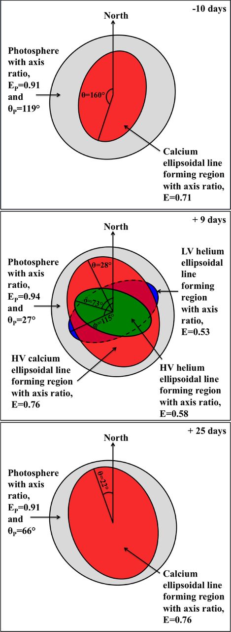
A schematic of the simulated line-forming regions at −10 (top), +9 (middle) and +25 d (bottom) for Ca ii (red) and LV He i (blue) and HV He i (green) covering an ellipsoidal photosphere with an axis ratio, EP and aligned with the long axis at θP from North (grey). The polarization simulation was able to successfully reproduce the observed continuum and line Stokes vectors.
For the data at −10 d, we found that a configuration of an ellipsoidal photosphere with EP = 0.91, with the major axis oriented at θP =119° reproduced the degree and angle of the continuum polarization. Simulations of the data at +9 and +25 d required the photosphere to be rotated to θP =27°, but with a similar axial ratio as used for the earlier epoch.
At −10 d, the polarization of Ca ii ir3 was best reproduced with an ellipse with an axis ratio of 0.71 and major axis oriented at θ ∼ 160°, offset by 41° from that of the photosphere. In terms of axis ratio, the simulated HV Ca ii did not undergo a significant change between −10 and +9 d, however the orientation of the region rotated by ∼130° (or −50°) to θ ∼ 30°. In order to recreate the larger fraction of photons absorbed by this line at +9 d, the size of the obscuring region was increased from 70 to 88 per cent of the major axis of the photosphere.
An ellipse with a more extreme axis ratio of 0.53 was required to reproduce the observed LV component of He i/Na i d, oriented at 115° and with size 75 per cent of the photosphere. This would imply that the LV He i component covers a substantially smaller portion of the photosphere than HV Ca ii and that the degree of asymmetry is more extreme. The polarization properties of the HV component of He i/Na i d could also be reproduced with an elliptical line-forming region with an axis ratio of 0.58. The lower absorption depth of the HV component implies that it covered less of the photosphere than the LV component, with a major axis 60 per cent of the size of the photosphere. The principal axis of the HV component line-forming region is also significantly rotated from that of the HV Ca ii line-forming region and the photosphere by 73° (or 42° from the LV He i/Na i d component).
The simulation indicates that neither the photosphere nor the Ca ii line-forming regions are subject to a dramatic change in geometry between +9 and +25 d. As there is a small scatter in the polarization angle between all species at these epochs, it is reasonable to expect that they may all have a geometry similar to that shown in Fig. 8.
We caution that while our assumption of line-forming regions composed of simple shapes can reproduce the observed levels of polarization, it does not imply that these are unique solutions nor that they are necessarily correct. In addition, the geometries for the line-forming regions we have identified using our toy model are also dependent on the choice of the ISP.
5 DISCUSSION
5.1 iPTF 13bvn in the context of other stripped CCSNe
iPTF 13bvn stands out amongst the limited sample of stripped-envelope CCSNe for which there are polarimetric observations, by having such a dense time series of spectropolarimetric observations (six epochs). The observed polarization properties of this class of SNe are very diverse, particularly regarding the line polarization. iPTF 13bvn shows similarities to the other stripped-core SNe, however there are also some aspects in which it exhibits significantly different behaviour.
The low levels of continuum polarization observed here are consistent with those found in other stripped CCSNe, such as SNe 2008D, 2007gr, 2005bf, and 2002ap (Kawabata et al. 2002; Maund et al. 2007a; Tanaka et al. 2008; Maund et al. 2009). These levels of polarization limit the degree of global asymmetries to ≲10 per cent (Höflich 1991). A feature consistently observed in all stripped CCSNe (Maund et al. 2009), and some thermonuclear Type Ia SNe (Mazzali et al. 2005), is the absorption trough of Ca ii ir3 , which is commonly associated with high velocities (∼10–20 000 km s−1) and large degrees of polarization (∼2–4 per cent). This feature tends to form at higher velocities in the ejecta and with a polarization angle that is markedly different to those of other species (Maund et al. 2007a,b; Tanaka et al. 2008; Maund et al. 2009; Tanaka et al. 2012). In addition, occasionally separate LV and HV components can be resolved in the Ca ii line profile in the flux spectrum (e.g. Maund et al. 2009). Species such as He i, Fe ii, O i, Si ii and Na i d are frequently observed to form closer to the photosphere and with similar polarization angles that are distinct from that of Ca ii (e.g. SN 2008D; Maund et al. 2009, and their fig. 11). For iPTF 13bvn, the velocity at the Ca ii ir3 absorption minimum is substantially higher than that of the other species. At maximum light and a week later, the polarization angle at maximum polarization for Ca ii ir3 is different from He i and Fe ii. The multi-epoch observations here allow us to follow the temporal evolution of the polarization associated with spectral lines. In iPTF 13bvn, both Ca ii and He i are observed to have photospheric and HV components that are geometrically distinct. Fe ii λ4924 is also polarized at similar velocities and has a similar orientation the HV He i and Ca ii line-forming regions, which is unique to iPTF 13bvn.
The only Type Ib SNe with spectropolarimetric observations, other than iPTF 13bvn, are SNe 2005bf, 2008D and SN 2009jf (Maund et al. 2007a, 2009; Tanaka et al. 2012). Maund et al. (2007a) presented polarimetric observations of the unusual SN 2005bf that was originally classified as a Type Ic SN (Morrell et al. 2005), before the later appearance of He lines (Folatelli et al. 2006). For SN 2008D, Maund et al. (2009) presented two epochs of spectropolarimetry at ∼V-band maximum and 15 d later. At the closest comparable epochs of 0 and +25 d, SN 2008D shows similarities to iPTF 13bvn in the polarization associated with certain spectral lines. For SN 2008D, the velocities and polarization angles at the absorption minimum of He i and Fe ii lines indicates that the two species are found in similar parts of the ejecta, while Ca ii is found at higher velocities and separated in polarization angle by ∼100°. iPTF 13bvn shows similar behaviour to SN 2008D at 0 d, where He i and Fe ii are observed to have similar polarization angles at similar velocities, while Ca ii ir3 is observed at a higher velocity with a polarization angle offset from the other species by ∼70°. Maund et al. (2009) also observe significant polarization associated with the O i λ7774 line, the polarization angle of which aligns with that of HV Ca ii at V-band maximum. For iPTF 13bvn, however, O i λ7774 appears much later and there is no significant polarization associated with it until +36 d, at which stage the polarization angle is aligned with the continuum and all other polarized species. Maund et al. (2009) also found a polarization maximum around 6200 Å which they attribute to a blend of Si ii and an HV component of H α at −17 050 km s−1. Similarly to iPTF 13bvn, the feature had also disappeared by the later epoch.
5.2 Complex multi-axis symmetry
The spectropolarimetric data of iPTF 13bvn have revealed the presence of multiple separately polarized components to the ejecta. The observations of loops on the q–u plane indicate that the orientation of the line-forming regions for Ca ii ir3 and He i/Na i d change with velocity (radius). The loops observed at +9 d and the step-like discontinuities in the polarization angle across the Ca ii ir3 and He i/Na i d profiles at +7 and +9 d imply that there are two geometrically distinct line-forming regions for the LV and the HV components.
The LV components of He i and Ca ii ir3 have the same polarization angle, implying that they form in the same location in the ejecta. These separately polarized components may suggest either two physically distinct line-forming regions for both calcium and helium or a change in the underlying ionization structure (Chugai 1992). The possible geometry of LV He i, from the Monte Carlo simulations, may then also be applicable to LV Ca ii. Although we have assumed simple ellipsoidal configurations for the line-forming region, and have not explored more complex geometries, we can rule out some geometric configurations. The rotation of the polarization angle across these lines, compared to the continuum polarization angle, shows that a shell with a similar shape to the photosphere that selectively blocks only part of the unpolarized light cannot be responsible for the observed degree of polarization (Kasen et al. 2003). The small scatter in the polarization angle across the LV components also suggests that this shared line-forming region is a single continuous structure in the ejecta, rather than arising in clumps (Hole, Kasen & Nordsieck 2010; Maund et al. 2010). In terms of the simple geometries explored in the simulation here and those presented by Kasen et al. (2003) and Hole et al. (2010), a non-clumpy elliptical line-forming region or shell, with different orientations to the asymmetry of the photosphere, can provide a reasonable explanation for the observed polarization properties of iPTF 13bvn. Previously, Maund et al. (2007a) inferred spherical configurations for the LV line-forming regions for SN 2005bf. In addition, although the jet-torus paradigm (Khokhlov et al. 1999) has been invoked to explain spectropolarimetric observations of some stripped CCSNe (Tanaka et al. 2008), we can exclude a torus-like line-forming region for the LV components as we do not observe the high levels of polarization predicted for such a geometry (Kasen et al. 2003).
The HV component of Ca ii ir3 in iPTF 13bvn is observed to be highly polarized, with a velocity much greater than the bulk of the ejecta. For iPTF 13bvn, we observe the same polarization angle in HV Ca ii, HV He i and Fe ii, which is in stark contrast to the distinctly different polarization angle for Ca ii ir3, compared to other species, observed for SNe 2005bf, 2007gr and 2008D (Maund et al. 2007a; Tanaka et al. 2008; Maund et al. 2009). Similarly to the LV component, the polarization properties of HV Ca ii were best replicated in the polarization simulation with an elliptical line-forming region. It is interesting to note that the presence of two velocity components for Ca ii ir3 is only discernible in the spectropolarimetric data, and that these two components are not resolved in the line profile of the flux spectrum. This undermines the accuracy of our simulation, which assumes that the line depth and polarization were due to the same line-forming region. The 2D bipolar model of Tanaka et al. (2012) produces a straight line on the q–u plane which also provides a match to the observed polarization characteristics of HV Ca. It is unclear to what degree Na i d plays a role in the He i/Na i d blend, and therefore whether He i and Ca ii share the same line-forming region. The results of the polarization simulation suggest that, likewise, an elliptical line-forming region can also reproduce HV He i but that is rotated compared to HV Ca ii.
In the later epochs, (+25 and +36 d) the loops on the q–u plane across the He i/Na i d blend and Ca ii ir3 profile (Fig. 4) appear more variable with several peaks in the degree of polarization apparent in Fig. 1. The evolution across the line is reminiscent of those generated in the simulations by Hole et al. (2010), where the ejecta are composed of clumps separated in velocity space. This suggests that the ejecta, while apparently still following a principal axis of symmetry, develop a degree clumpiness at later times. At −10 d, the line polarization of the LV and HV component share similar polarization angles consistent with a single axial symmetry, with no evidence of clumpiness within the ejecta. The implication is that between +9 and +25 d the ejecta became clumpy, most likely due to hydrodynamic instabilities. Such instabilities could propagate through the ejecta (Blondin & Ellison 2001) or may develop from remnant asphericities in the explosion mechanism itself, such as the standing accretion shock instability (Janka et al. 2007) or through the propagation of a jet-like flow through the progenitor star (Couch, Wheeler & Milosavljević 2009, see also Wheeler, Maund & Couch 2008 for discussion of jet-induced hydrodynamical instabilities in SNR Cas A and Hammer, Janka & Müller 2010 for simulations of instabilities in SN explosions).
There are no previous observations of two geometrically and physically distinct He i line-forming regions in the ejecta of Type Ib SNe. The properties of both the HV and LV components for iPTF 13bvn are different from those observed for other stripped CCSNe. It is possible that the scarcity of previous polarimetric observations or viewing angle effects may have meant that this feature has been missed in the other SNe. If these features are truly unique to iPTF 13bvn, signs of the SN's peculiarity may be expected in the light curve or spectra. iPTF 13bvn was classified as a Type Ib SNe, with similarities to SN2009jf, while the light curve was observed to be fast declining and of low luminosity (Srivastav et al. 2014). It is possible that the observations of the two He i components are related to the plateau in the evolution of the He i velocity (see Fig. 2). A similar plateau is also observed in SN 2008D (see Modjaz et al. 2009, and their fig. 13), however the polarized HV and LV components in Ca ii and He i observed in iPTF 13bvn are not seen in SN 2008D (Maund et al. 2009). Only increasing the sample of Type Ib SNe with high polarimetric coverage can resolve the question of whether this complex ejecta morphology is common to all Type Ib SNe or only a subset, and what role the explosion mechanism plays in the formation of these multiple components.
5.3 Non-thermal excitation
The velocity at the absorption minimum of the He i/Na i d blend is observed to decay steeply before plateauing at around maximum light (see Fig. 2). The velocities measured for the He i λλ6678, 7065 lines also appear to plateau at the same time (see Fremling et al. 2014, and their fig. 6). The plateau in the He i velocity may arise from non-thermal excitation, from the direct deposition of gamma rays from the radioactive decay of 56Ni and 56Co, at velocities higher than the photospheric velocity (Lucy 1991). The geometry of He i may, therefore, serve to trace the geometry of the radioactive nickel. The coincident emergence of the HV and LV components in the polarimetry with the beginning of the He velocity plateau at ∼ maximum light suggests that the non-thermal excitation of the He i lines also powers those components.
In principle, the collision of an approximately spherical ejecta with an aspherical circumstellar medium (CSM) could also produce the observed early evolution in the polarimetry. If interaction were the dominant source of non-thermal excitation, we might expect to also see narrow emission lines in the spectrum, which are not seen in our observations of iPTF 13bvn. Furthermore, the collision of ejecta and a CSM would result in an injection of energy, identifiable in the light curve as a decline that is slower than expected from radioactive decay. Srivastav et al. (2014) note, however, that iPTF 13bvn has a faster decline than most Type Ib/c SNe and faster than expected for the decay of 56Co. This suggests a deficiency of energy in the ejecta due to incomplete trapping of gamma rays as opposed to energy from interaction with the CSM. The observations, therefore, disfavour interaction as the source of the separate components and the He i velocity plateau and are, instead, consistent with 56Ni located above the photosphere at and after the light-curve maximum. The photospheric velocity measured at 18 d post-explosion reveals that nickel must be mixed out to ∼50–65 per cent of the ejecta, by radius, at ∼8700 km s−1. Bersten et al. (2014) performed one-dimensional hydrodynamical explosion models of iPTF 13bvn which required 56Ni to be mixed out to ∼96 per cent of the initial mass of the progenitor to reproduce the observed rise time of the light curve. The discrepancy between these two estimates for the degree of Ni mixing most likely arise in the application of a 1D model assuming spherical symmetry to, as we have observed, an asymmetrical situation. If the polarization of the HV and LV He i components at +7 and +9 d trace the 2D projected distribution of nickel, this implies that not only is it not spherically distributed, covering only a portion of the photosphere, but also that it is distributed in at least two (if not more) outflows originating from the core. Our observations have demonstrated the importance of spectropolarimetry for measuring how Ni is mixed into the outer layers of the SN ejecta and the degree of this mixing. This has important implications for how photometric and spectroscopic observations are interpreted, especially in the context of 1D models.
5.4 Implications for the explosion geometry
The absence of any strong O i lines in the spectrum until +25 d indicates that the core is still shielded by the photosphere until that epoch. The presence and polarization of He i, at ∼ maximum light, indicates the role of non-thermal excitation from Ni deposited above the core by an axisymmetric outflow that stalled in the helium mantle.
The approximate alignment of the continuum polarization angle in the later epochs (+25 and +36 d) with that of the HV component suggests that there is a principal axis of symmetry for the explosion which may lend itself to the interpretation of a bipolar or jet driven explosion. In this model a jet, originating either from asymmetric neutrino emission (Blondin & Mezzacappa 2007) or the magnetorotational mechanism (LeBlanc & Wilson 1970; Mikami et al. 2008), would carry heavy elements in bipolar flows, while low- and intermediate-mass elements (e.g. helium and oxygen) would form a torus in the equatorial plane (Khokhlov et al. 1999; Khokhlov & Höflich 2001; Maeda et al. 2002). We observed no such segregation between the locations of heavier mass (iron and calcium) and lower mass (helium and oxygen) elements in the ejecta, that would suggest such a geometric configuration for iPTF 13bvn. The presence of a separate LV component of He i , which must also arise from non-thermal excitation, also implies that the distribution of nickel cannot be described by just a simple bipolar geometry.
In comparison with the velocity of the HV He component (∼−8700 km s−1) which we use as a tracer for the Ni distribution, the high velocities (∼−13 000 km s−1) measured for Fe ii lines at early times implies these features arise from primordial iron already present in the envelope of the progenitor. Likewise, the LV inferred for the Ni makes it improbable that the Ca ii ir3 HV component traces a fast moving jet. The deposition of nickel outside of the photosphere, at ∼ maximum light, would lead to significant losses of gamma-ray photons, which would otherwise be trapped in the ejecta under the photosphere. This could explain the low-luminosity and fast light curve decline of iPTF 13bvn (Srivastav et al. 2014), and may also imply that the nickel mass derived from the bolometric light curve (0.05–0.1 M⊙; Bersten et al. 2014; Srivastav et al. 2014) may underestimate the true value.
Previously, the action of bipolar flows has been inferred from spectropolarimetry of other CCSNe. Tanaka et al. (2008) observed HV Ca in the Type Ic SN 2007gr, which they proposed was formed in a bipolar outflow, with oxygen distributed in a torus in the equatorial plane. Polarization in the wavelength region around the Ca ii ir3 in the Type Ic SN 2002ap was interpreted by Kawabata et al. (2002) as indicating the presence of a relativistic jet (0.115c) that had punched through the ejecta. Later, Wang et al. (2003) presented three epochs of spectropolarimetry of SN 2002ap and challenged this interpretation, suggesting the polarization was associated with oxygen at much lower velocities and suggested the data were consistent with a bipolar jet-like flow that had stalled in the core. Similarly, Maund et al. (2009) invoked a thermal energy dominated jet-like flow, that had stopped within the core, to explain the orthogonality between the polarization angle of HV Ca ii with the angles of helium and iron at lower velocities in the Type Ib SN 2008D. Maund et al. (2007a) also favoured a jet, that stopped above the core in the helium mantle, for the Type Ib/c SN 2005bf. Mauerhan et al. (2015) also favour plumes of radioactive nickel to explain the polarization of the Type IIb SN 2011dh. Maund et al. (2009) and Wang et al. (2003) predicted that, as the photosphere recedes through the deeper layers, later observations of Type Ibc SNe would reveal evidence of an asymmetric flow originating from the explosion. Our multi-epoch spectropolarimetry of iPTF 13bvn has confirmed these predictions. Although there are differences between iPTF 13bvn and these other Type Ibc SNe, overall a consistent picture of the geometry of these events is emerging.
The geometrical properties inferred here are reminiscent of the complex morphology of the Galactic Type IIb SN remnant Cas A. The presence of the opposing north-east ‘jet’ and south-west ‘counter-jet’ are indicative of axisymmetric bipolar flows associated with the explosion, similar to that inferred here for the observations at later epochs. Several authors agree, however, that these so-called ‘jets’ are secondary features, perhaps arising due to instabilities (Wheeler et al. 2008), accretion on to a neutron star (Janka et al. 2005) or due to precession of the axis of rotation when the bipolar flows were launched (Burrows et al. 2005). Similarly, Milisavljevic & Fesen (2013) conclude that while the observed jets are unlikely to be the result of a jet-induced explosion they are intrinsic to the explosion. Wheeler et al. (2008) proposed a model in which the jet-induced explosion launched products from explosive nucleosynthesis in a jet in the south-east direction, not along the NE/SW axis. Blondin, Borkowski & Reynolds (2001) and Milisavljevic & Fesen (2013) interpreted the presence of several large ejecta rings surrounding iron-rich ejecta to be due to the non-axisymmetric deposition of nickel in clumps in the explosion and such a scenario has also been proposed for SN 1987A (Li, McCray & Sunyaev 1993). The inference of two outflows of nickel and additional ‘clumps’ or ‘bubbles’ of nickel in iPTF 13bvn may therefore have very real analogues in resolved SN remnants like Cas A (Milisavljevic & Fesen 2015).
5.5 Polarimetric evolution and the implications for the progenitor system
The possible identification of a progenitor candidate for iPTF 13bvn, as reviewed in Section 1, has generated debate over the progenitor system that gave rise to this SN. For iPTF 13bvn, we have identified three main axes of symmetry over the period covered by our spectropolarimetric observations corresponding to: the HV component at +9 d and the line and continuum polarization in the later epochs at ∼135°; the LV component at +9 d at ∼25°; and the alignment of the line polarization angles of multiple species at the earliest epoch of −10 d at ∼75°. The asymmetries in the earlier epochs reflect the shape of the outer most layers of the ejecta. The difference in the polarization angles observed at −10 d and those at later epochs (+25 and +36 d) suggests that the outer layers of the ejecta did not share the same geometry as the explosion. This suggests, similarly to what has been observed for Type IIP SNe arising from red supergiant progenitors (Leonard et al. 2006; Chornock et al. 2010), that the envelope of the pre-SN star must have been sufficiently large in order to conceal the inner explosion asymmetries for 18 d (until 0 d when evidence of the inner explosion geometry began to emerge).
In the context of understanding the origin of the geometry of the outermost ejecta, the identification of the polarized absorption feature at ∼6200 Å becomes especially interesting. The feature is significantly polarized in the first two epochs only (−10 and 0 d) before both the degree of polarization and absorption depth decrease. As has been suggested for other Type Ib SNe (Wheeler et al. 1994; Deng et al. 2000; Branch et al. 2002; Parrent et al. 2015), if this feature is H α at −16 400 km s−1, this would imply that the H line-forming region lies in the outermost layers of the ejecta, perhaps in a shell at the outer edge of the ejecta, as was suggested for Type Ib SN 2008D (Maund et al. 2009). The polarization of this feature may then reflect asymmetries in the outermost layers of the progenitor or the progenitor's wind swept up by the ejecta, as has been proposed for some Type IIb SNe. The polarization angle of the 6200 Å feature is consistent with those of the rest of the species at −10 d, in contrast to the H α polarization of Type IIb SN 2001ig, where it is found to have a different distribution within the ejecta compared to the dominant axis (Maund et al. 2007c). Similarly, Chornock et al. (2011) found that the H α polarization was aligned with that of He i λ5876 but rotated with respect to Ca ii and Fe ii for transitional Type IIb/Ib SN 2008ax. In contrast to the modest polarization of ∼0.6 per cent found here, Chornock et al. determined large variations of ∼3 per cent across H α, indicating large asphericities in the outer ejecta. SNe 1993J and 1996cb showed more modest polarization across H α of ∼1.5 per cent (Tran et al. 1997; Wang et al. 2001). For SN 2011dh, Mauerhan et al. (2015) found that the polarization of enhanced line polarization associated with H α peaked at 30 d post-explosion and aligned with the continuum polarization at early times. This, however, was not related to the shape of the outer layers of the ejecta but due to plumes of 56Ni deposited outside of the photosphere according to Mauerhan et al. (2015). In general, the polarization properties of H α in Type IIb and Ib SNe are quite different which may imply distinctly different progenitor configurations for the two types of SNe
The shape of the outer layers of the SN ejecta is also subject to the geometry of the shock break out, which is dependent upon the geometry of the explosion and dynamics of the interaction of the shock front as it propagates through the progenitor star. The post-maximum polarization properties indicate that the explosion of iPTF 13bvn was highly asymmetric. Matzner, Levin & Ro (2013) performed calculations which showed that the resulting shock front of an aspherical explosion may emerge at an oblique angle to the stellar surface. A key prediction of these models is this would induce large asphericities in the highest velocity material and hence significant polarization. At later times, the polarization angles are then predicted to rotate, as the geometry becomes progressively dominated by the shape of the explosion mechanism, as we have observed for iPTF 13bvn. The emergence of the explosion geometry at 0 d (18 d post-explosion) implies the progenitor of iPTF 13bvn must have had a relatively extended envelope, which argues against oblique shock break out as the source of the early polarization that Matzner et al. (2013) determined is more easily produced by compact progenitors, such as WR stars.
The early polarization may also arise in a distorted stellar envelope. Tidal distortion of the progenitor star as a result of binary interaction has been discussed as the source of the observed polarization in numerous Type IIb SNe including SN 1993J and recently in SN 2011dh by Mauerhan et al. (2015). Tran et al. (1997) and Trammell et al. (1993) observed high levels of continuum polarization in SN 1993J, of p ∼ 1–2 per cent which exhibited no strong temporal dependence. Höflich (1995) found that this could be produced by an oblate model with an axis ratio of 0.6, while Tran et al. (1997) and Trammell et al. (1993) argued that the lack of strong temporal change in the polarization was an indication that the asymmetry was not intrinsic to the explosion but due to a distorted envelope. The strong asphericity was linked to a pre-SN common envelope phase in a close binary system (Höflich 1995). Similar polarization properties were observed for SN 1996cb (Wang et al. 2001) and SN 2001ig (Maund et al. 2007c), with Maund et al. (2007c) suggesting that they were the result of a similar binary progenitor system. The alignment of the Ca ii ir3, Fe ii and Si ii polarization angles and the non-zero degree of continuum polarization (∼0.2–0.7 per cent depending on the chosen ISP) suggests that the envelope was distorted in an axisymmetric manner. The effect of the tidal distortion of the progenitor on the early-time polarization of the SN may be amplified by how the explosive shock is able to propagate through the distorted star. Fast rotation or tidal interaction with a binary companion leads to a density profile in the progenitor that is steeper along the direction of the poles. Steinmetz & Höflich (1992) showed that a spherical shock front would take on a prolate shape upon encountering the steeper density gradient along the poles. For a massive, differentially rotating star (like the progenitor of SN 1987A), Steinmetz & Höflich (1992) found that at ∼30 d post explosion the photosphere receded through the oblate ejecta to the prolate regions, producing a rotation of the polarization angles. The observations of iPTF 13bvn are also roughly consistent with this model.
Spectropolarimetric surveys of Galactic and Large Magellenic Cloud (LMC) WR stars show that the majority (∼80 per cent) are slow rotating spherically symmetric stars (Harries, Hillier & Howarth 1998; Vink 2007; St-Louis 2011). Based on geometry alone, the progenitor of iPTF 13bvn is unlikely to have been a slowly rotating WR star. Vink, Gräfener & Harries (2011) and Gräfener et al. (2012) discovered that a subset of WR stars that were rotating sufficiently fast to result in a flattened wind were also associated with ejecta nebulae, such that they concluded that these had to be young WR stars (having recently been through a luminous blue variable or red supergiant phase). In low-metallicity environments, the line-driven winds of these fast rotators will be too weak to remove significant amounts of angular momentum (Yoon & Langer 2005), such that they would retain any rotational induced asymmetries up to the point of explosion. Vink (2007) proposed that this effect was at most limited to metallicities below that of the LMC. Kuncarayakti et al. (2015) measured the metallicity of the region of iPTF 13bvn as being slightly subsolar, which would suggest as WR star in this region would not be expected to explode as a distorted, fast rotator.
The polarimetric observations may be more easily explained in the context of the close binary model proposed by Bersten et al. (2014). The explosion of a low-mass He star in a binary system does not require the compactness implied by the explosion of a single massive WR star. Indeed Bersten et al. (2014) showed that the non-detection of shock cooling in the early light curve (Cao et al. 2013), does not preclude the existence of an extended envelope and find the radius of the progenitor may be as large as R ≲ 150 R⊙. Kim, Yoon & Koo (2015) also find that the pre-explosion photometry can be replicated with a helium star progenitor of 3.0–4.4 M⊙ (with an O-type star companion) and extended radius of ∼12–30 R⊙. Interestingly, stars in this mass range are expected to undergo mass transfer (Case BB) in the final decades before core collapse (Yoon, Woosley & Langer 2010). In this case, the extended helium envelope of the star would be significantly distorted, having filled a Roche Lobe that deviates dramatically from spherical symmetry. In addition, stars in this mass range (3–3.8 M⊙) are also predicted to retain a residual amount of hydrogen in the outermost layers (Yoon et al. 2010). Synthetic spectra of SNe resulting from the explosion of stars in this range exhibit H i lines at early times up until peak (Dessart et al. 2015), similarly to the absorption feature at ∼6200 Å observed in iPTF13bvn. The polarimetry may then support the explosion of a star with final mass of 3–3.8 M⊙ with a recent binary interaction phase. Questions remain, however, as to whether the distortion of the helium envelope from mass transfer in the previous decades would be preserved up until core collapse and through to the observations at −10 d. Nevertheless, the mass transfer would result in a complex CSM from which the early polarization may result. It should be noted that mass transfer during carbon-oxygen core contraction with residual hydrogen remaining in the envelope is predicted only within a narrow mass range. Should the progenitor mass be several times higher than the estimates of a few solar masses, which Wheeler et al. (2015) suggest could be the case, the evolutionary paths will be vastly different and a significantly distorted Roche Lobe in the final decades of the star's life may not be expected.
In summary, our polarimetric observations favour an extended, distorted progenitor (possibly with residual H in the outer layers) rather than a compact WR star.
6 CONCLUSIONS
We find iPTF 13bvn to have exhibited significant continuum and line polarization in observations covering the period from −10 to +36 d, with respect to the r-band light-curve maximum. The continuum was intrinsically polarized at the 0.2–0.4 per cent level throughout the observations, implying asphericities of ∼10 per cent in the shape of the photosphere. The degree and angle of continuum polarization was found to be dependent on the choice of the ISP.
Significant polarization was found to be associated with the absorption profiles of spectral lines of Ca ii ir3, He i/Na i d, He i λλ6678, 7065, Fe ii λ4924, Si ii λ6355 and O i λ7774. The Ca ii ir3 absorption showed the strongest degree of polarization of ∼3 per cent at +25 d. The polarizations of the He i/Na i d and Fe ii reached maximum levels of ∼1 per cent, followed by O i and Si ii/H α at ∼0.6 per cent. We propose that the observation of two loops on the q–u plane associated with the He i/Na i d profile at +7 and +9 d indicates the presence of at least two physically distinct components to the ejecta. The formation of separate loops due to the blending of Na i d with He i was considered unlikely due to the sharp discontinuity observed in the polarization angle across the profile and the lack of evidence of a strong contribution to the blend from Na i d at +7 and +9 d. Both loops are attributed to He i. Similarly, Ca ii also show a ‘step-function’-like trend in the evolution of the polarization angle with velocity, supporting the interpretation of at least two distinct line-forming regions for He i and Ca ii in the ejecta. The LV components of Ca ii and He i were found to share the same polarization angle implying a shared line-forming region for the two ions. The HV components were observed with polarization angles separated by ∼40°.
The simultaneous emergence of the HV and LV components in the polarization data with the onset of the He velocity plateau indicated the presence of non-thermal excitation. The polarization of the HV and LV He i components was used to trace the 2D projected distribution of nickel in the ejecta, and suggests the presence of at least two outflows originating from the core. We are able to constrain the bulk of nickel to lie interior to ∼50–65 per cent of the ejecta radius, at a velocity of ≲8700 km s−1. This is in disagreement with the prediction from 1D hydrodynamical models, requiring mixing out to ∼96 per cent of the initial mass of the progenitor to reproduce the observed rise time of the light curve.
The approximate alignment of the continuum polarization angle in the later epochs with that of the HV component suggests that there was a main axis of symmetry in the explosion, which could be consistent with a bipolar or jet-driven explosion. The high quality of our data reveal, however, that the structure of the ejecta is not just described by a simple, single axial symmetry and that the morphology of the explosion is much more complicated. Other outflows, originating from the explosion, appear to have been launched in multiple directions but, similarly to other Type Ib SNe, stalled in the He mantle of the progenitor star. The structure of the outer layers of the ejecta are consistent with a rotationally supported, non-WR star that had retained a thin shell of H at the time of explosion. Our spectropolarimetric observations of iPTF 13bvn have revealed a complex explosion geometry that is reminiscent of that observed in the Galactic SN remnant Cas A.
The authors would like to thank the anonymous reviewer for their careful examination of this manuscript and the comments which helped to improve it. We are also grateful to Professor S.-C. Yoon for helpful comments on a draft of the manuscript. ER is supported through a PhD studentship awarded by the Department of Education and Learning of Northern Ireland. The research of JRM is supported through a Royal Society University Research Fellowship. JCW is supported by NSF Grant AST 11-09881. JMS is supported by an NSF Astronomy and Astrophysics Postdoctoral Fellowship under award AST-1302771. The authors are grateful to the ESO for the generous allocation of observing time. They especially thank the staff of the Paranal Observatory for their competent and never-tiring support of this project in service mode.
Based on observations made with ESO Telescopes at the Paranal Observatory, under programme 091.D-0516.
iraf is distributed by the National Optical Astronomy Observatories, which are operated by the Association of Universities for Research in Astronomy, Inc., under cooperative agreement with the National Science Foundation – http://iraf.noao.edu/.
REFERENCES
