


Abstract
The results of the in situ exploration of the asteroid (4) Vesta by the Dawn spacecraft open new perspectives in the field of interpretation of remote-sensing polarimetric measurements of asteroids. (4) Vesta has long been known to be the only asteroid exhibiting a cyclic variation of the degree of linear polarization of the sunlight scattered by its surface, with a period which is synchronous with the object's rotation. This variation must be the consequence of some heterogeneity of the asteroid's surface, including regions characterized by different albedo, or composition, or regolith properties, or a combination of the above features. For a long time, this kind of conclusion has remained essentially qualitative. Now, after the extensive exploration of Vesta's surface by Dawn, it is possible to interpret the data set of polarimetric measurements of Vesta, including some unpublished data presented here for the first time, in terms of a correspondence between the degree of linear polarization and the variation of local properties of the surface visible to ground-based observers during Vesta's rotation, as seen at different epochs and under different illumination conditions. This makes it possible to refine our knowledge of the empirical relation between polarization properties and albedo, which is commonly used to derive the albedo from remote-sensing measurements of linear polarization of atmosphereless Solar system bodies.
1 INTRODUCTION
(4) Vesta is the only asteroid for which a periodic variation of the degree of linear polarization of the sunlight scattered by the surface has long been convincingly found to occur (Gradie, Tedesco & Zellner 1978; Dollfus & Zellner 1979; Lupishko et al. 1988). Some authors mention the possible detection of a weak polarimetric modulation for a few other objects, including (7) Iris (Broglia & Manara 1990), (16) Psyche (Broglia & Manara 1992) and (1943) Anteros (Masiero 2010), but Vesta is the only asteroid for which this phenomenon has been convincingly demonstrated and confirmed at different epochs, including the very recent analysis carried out by Wiktorowicz & Nofi (2015). According to pioneering observations carried out in the 1970s (Degewij, Tedesco & Zellner 1979, and references therein), the degree of linear polarization of Vesta was found to exhibit a sinusoidal variation with a period synchronous with rotation. The degree of polarization turned out to be anticorrelated with the photometric light curve, the maximum of polarization being reached at the minimum of the light curve, and vice versa. This finding was later confirmed also by Lupishko et al. (1988). The discovery of this phenomenon led the observers to correctly infer for Vesta a rotation period of 5.342 h, and to rule out a period twice as long, also compatible with available photometric data. The latter would correspond to a photometric light curve exhibiting two maxima and minima, as would be expected for any object whose periodic luminosity variation is due mostly or exclusively to shape effects. Conversely, the photometric variation of Vesta seemed to be largely dominated by albedo variegation, rather than by shape effects (Dollfus & Zellner 1979). Cellino et al. (1987) collected all light curves of Vesta available at that time, and showed that they were compatible with a model based on the idea that the overall shape of the object is that of an oblate spheroid, the shape expected for Vesta assuming that it is in hydrostatic equilibrium, and that the photometric variation is due to the presence of a large, hemispheric-scale ‘albedo spot’. This model was in good agreement with photometric and polarimetric evidence available at that time.
The spectroscopic confirmation (Binzel & Xu 1993) of the existence of a large dynamical family of small asteroids, having proper orbital elements very similar to those of Vesta (Zappalà et al. 1990), seemed to be another confirmation of the above interpretation. In this scenario, the large albedo spot on Vesta's surface could be interpreted as corresponding to some very large impact crater produced by the energetic impact which created the dynamical family.
HST images of Vesta (Thomas et al. 1997) found evidence of the presence of a large crater on the Southern hemisphere, although they also suggested that the albedo variegation could be more complex than previously assumed, and not strictly corresponding to the location of the large impact crater. Moreover, the overall shape was found to slightly depart from that of an ideal spheroid, with evidence of a mild overall triaxiality.
Images of Vesta obtained by the Dawn spacecraft (Russell et al. 2013) give now a detailed description and overall explanation of the physical properties and of the thermal and collisional history of this asteroid. The main findings relevant for this work are given in Section 2. Here we mention the presence of two impact basins, one on top of the other, named Rheasilvia and Veneneia (Jaumann et al. 2012). Rheasilvia, the younger of these two craters, is about 1 Gy old (Marchi et al. 2012). It is centred at 301° W, 75° S, roughly 15 deg from the South Pole, and has a diameter of 500 ± 25 km (Schenk et al. 2012). Veneneia is centred at 170° E, 72° S, has a diameter of 400 ± 25 km (Schenk et al. 2012), but it has been half destroyed by Rheasilvia.
According to the recent analysis of asteroid families by Milani et al. (2014), the structure of the Vesta family in proper element space is complex and actually suggests the presence of at least two major impact events. A more recent analysis by Spoto, Milani & Knežević (2015) gives ages of about 930 and 1900 Myr for the two impact events. The first value is fully compatible with the age of Rheasilvia as proposed by (Marchi et al. 2012). The second value, plausibly corresponding to the Veneneia event, is indicative of an event occurred much earlier.
For polarimetric studies, the exploration of Vesta by Dawn is an invaluable resource to explain the polarimetric behaviour of this asteroid found by means of ground-based, disc-integrated measurements of its polarization state obtained at different rotation angles and in different illumination conditions. In other words, Dawn images of Vesta offer us a unique opportunity to obtain for the first time the ground truth in asteroid polarimetry: the possibility to link the polarimetric properties of an asteroid surface measured at different epochs by means of disc-integrated, remote observations, knowing the local properties of the fraction of the surface seen at each observation epoch. This provides for the first time the possibility to understand which surface properties are responsible for the observed variation of linear polarization measured by ground-based observers. This kind of analysis is possible in the laboratory using different samples of meteorite materials, but Dawn observations make it possible for the first time to study details of the surface of a single body, including composition heterogeneity, macroscopic roughness, overall texture and slope of its terrains.
Of course, this analysis requires observations covering sufficiently long time spans, to be able to follow the variation of the degree of linear polarization as different surface features become visible, or disappear, during the rotation of the asteroid. Let us call these polarimetric observations, covering a full, or nearly full rotational cycle, ‘polarimetric light curves’. We will use this term in this paper, but warn that this should not be confused with the usual photometric light curves.
The purpose of this paper is to carry out the first, extensive analysis of Vesta polarimetric data in such a way as to find some well-defined relation between the variation of the linear degree of polarization of the disc-integrated flux of sunlight scattered by the surface, and the visibility of well-defined features of Vesta's surface identified by Dawn images and spectrophotometric data. In so doing, we also obtain useful data for a better calibration of the currently adopted relations between asteroid albedo and disc-integrated polarimetric properties, to be extended to the study of other objects.
2 DAWN AT VESTA: A SHORT SUMMARY OF RESULTS
The Dawn probe, launched in 2007, reached Vesta in 2011 (Russell et al. 2012). Based on properties like mass (Konopliv et al. 2011), volume (Thomas et al. 1997) and reflectance spectrum (McCord, Adams & Johnson 1970) inferred from available ground-based observations, Vesta was expected to be a completely differentiated body having a metallic core and a basaltic-like crust, whose spectral properties have long been associated with those of howardite, eucrite and diogenite (HED) achondritic meteorites. Based on the data obtained by orbiting for one year around Vesta, Dawn confirmed the similarity between the crust of Vesta and the HEDs, while the gravitational field has been found to be consistent with a differentiated body having a core with a diameter above 200 km (Reddy et al. 2012; Russell et al. 2012; De Sanctis et al. 2012a).
A sidereal rotation period of 5.342 127 67 h, in agreement with, but much more accurate than previous estimates based on remote photometric observations, has been determined (Russell et al. 2012).
Two ancient impact basins, which have been named Rheasilvia and Veneneia, were found in the region of the South Pole of Vesta, in the location corresponding to the large southern basin already seen in HST images (Thomas et al. 1997; Jaumann et al. 2012). Large rings of grabens covering extended areas are associated with these two big craters (Jaumann et al. 2012).
The Dawn on-board spectrometer mapped the mineral distribution on Vesta (De Sanctis et al. 2011; Ammannito et al. 2013b; De Sanctis et al. 2013, see Fig. 1). As opposite to expectations based on the supposedly differentiated structure of Vesta, no evidence of large amounts of olivine (expected to be very abundant in the mantle's composition) has been found, neither on the surface or in the excavated craters. A relatively large amount of olivine was discovered only in the Northern hemisphere, far from the deeply excavated southern basins, while some very small and localized sites of enrichment of olivine have been only recently suggested (Ammannito et al. 2013a; Ruesch et al. 2014).
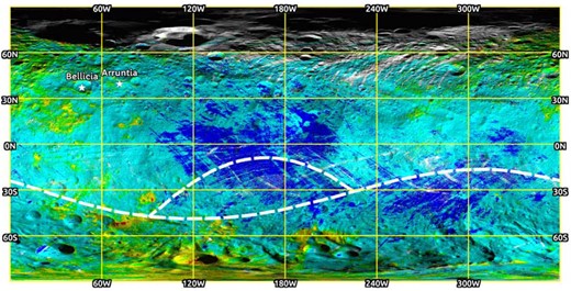
Map of lithologies found on the surface of (4) Vesta using the VIR instrument aboard the Dawn mission. Red colour is used to indicate diogenite, green corresponds to howardite, blue to eucrite. Yellow areas show regions with diogenite and howardite. Cyan areas show regions rich in eucrite and howardite. Two impact craters, Arruntia and Bellicia, which have been found to be rich in olivine, are also shown. The outlines of the two giant craters Rheasilvia and Veneneia, located close to the South Pole, are also noted (Ammannito et al. 2013a).
Vesta's spectrum has absorption features at 0.9 and 1.9 μm, indicative of Fe-bearing pyroxenes, similar to the spectra of HED meteorites (De Sanctis et al. 2012a). The mineralogy seems to have been strongly influenced by the huge impact that formed the Rheasilvia basin. Orthopyroxene-rich materials have been found in the deepest parts of the basin and within its walls. Large eucrite-rich regions are present at equatorial/mid-latitudes. Diogenitic lithology is exposed in a broad region extending from Rheasilvia to the Northern region (Ammannito et al. 2013b).
For the purposes of the present analysis, it is important to note that the global albedo map of Vesta obtained by Dawn shows large variations, and reveals the presence of different types of terrains (Li et al. 2013; Schroeder et al. 2013). It is also interesting that dark materials are sparsely present on the surface, with spectra often presenting an OH signature at 2.8 μm (De Sanctis et al. 2012b; McCord et al. 2012). Dark-rayed craters have been found, as well as buried dark materials which may suggest the delivery to Vesta of exogenic carbonaceous material (Reddy et al. 2012). No clear indication of phenomena of space weathering have been found on Vesta's surface (Pieters et al. 2012). Most surprisingly, however, some surface features seem to show evidence of processes related to the presence and possible flow of liquid water: gullies in the crater walls and pits in the crater floors (Scully et al. 2015). The presence of water, even if only transient, on the surface of Vesta, and the apparent lack of an olivine mantle were unexpected results. The origin of OH on Vesta may provide new insight into the delivery of hydrous materials in the asteroid main belt, and in the inner Solar system.
Dawn has evidenced a significant mineralogical variation of Vesta's crustal stratigraphy on local and global scales. Ejecta from large craters have distinct spectral behaviour, and materials exposed in the craters show distinct spectra on floors and rims. While these observations do not negate the earlier work based on the HED meteorites, they do add important new insight into the conditions under which Vesta formed and evolved.
3 POLARIMETRY OF ASTEROIDS
When the plane of polarization is parallel to the scattering plane Pr becomes negative, and this situation is named negative polarization. This usually occurs at phase angles between zero and about 20°. When the plane of polarization is perpendicular to the scattering plane the sign of Pr is positive, and we speak of positive polarization. Note that this is just a useful convention. The linear polarization is intrinsically a positive physical parameter. A sign of polarization is assigned in Solar system science just to concisely indicate both the degree of linear polarization and the orientation of the polarization plane.
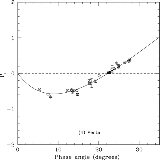
Polarization–phase curve of (4) Vesta. Full symbols correspond to a couple of measurements carried out at the Complejo Astronomico El Leoncito which have been published only recently by Gil-Hutton, Cellino & Bendjoya (2014). The other data points are taken from the PDS website.
It is important to note that the degree of polarization of the vast majority of the asteroids is found to be independent on other observing circumstances apart from the phase angle. Objects observed at the same phase angle, but at different epochs, give usually identical (within measurement uncertainties) values of linear polarization. One of the few exceptions is asteroid (4) Vesta, the subject of our present analysis, due to the dependence upon rotation of its degree of linear polarization. In this paper, we study this phenomenon resulting from available polarimetric light curves, each one obtained at a single (and generally different) value of phase angle.
4 AVAILABLE POLARIMETRIC DATA FOR VESTA AND NEW OBSERVATIONS
Being very bright, (4) Vesta has been extensively observed using all available techniques, including polarimetry, for many decades. We will not attempt here to include in our analysis an extensive use of the whole data set of single polarimetric observations of Vesta available in the literature. An updated phase–polarization curve of Vesta including all published measurements in the standard V filter is shown in Fig. 2. The shallow depth of the negative polarization branch, and the gentle slope h of the linear increase of linear polarization around the inversion angle are diagnostic of an object having a medium–high albedo. More in details, the inversion angle of Vesta is found to be around 23 deg of phase. The polarimetric slope h of Vesta has been found to have a value of about 0.0623 ± 0.0001 deg−1 (Cellino et al. 2015). According to the known relation between polarimetric slope and geometric albedo, this corresponds to a geometric albedo of the order of 0.30, the exact value depending on the adopted choice of the calibration coefficients of the slope–albedo relation. The albedo value found by thermal radiometry using IRAS data is significantly higher: 0.37 ± 0.02 (Tedesco et al. 2002), but this was based on one single observation, only. From Dawn data, it turns out that, apart from small-scale features which can exhibit more extreme variations, over large hemispheric regions the average geometric albedo may vary between values slightly lower than 0.29 up to values larger than 0.33 at the wavelength of 0.7 μm. In this paper, apart from some considerations that will be discussed in Section 6, our main goal is not to analyse the phase–polarization curve of Vesta shown in Fig. 2. The general variation of the degree of linear polarization at different phase angles concerns us mostly for another reason, namely that we can expect to get a stronger evidence of the existence of subtle, rotation dependent variations of polarization only when the measurements that we have at disposal have a good SNR. In turn, this most likely occurs at epochs when the linear polarization is intrinsically higher, rather than at epochs when the overall degree of polarization is much lower, namely, close to zero phase, or to the inversion angle.
What is most important for the purposes of the present investigation, is the variation of the linear polarization of Vesta as a function of rotation. For this reason, we focus our analysis on a small number of available polarimetric light curves obtained over the years by different authors. Due to the problems that we had in retrieving the original records of the timing of each measurement in this limited sample of available data (see discussion below), we did not even try to repeat this exercise in the case of the large number of single measurements obtained in other epochs (the ones shown in Fig. 2). Another reason is that in many cases these polarimetric data, as published by the observers, were plausibly nightly averages of several single measurements, obtained over time spans covering large fractions of Vesta's rotation.
The first simultaneous measurements of photometric and polarimetric light curves of Vesta (Degewij et al. 1979; Dollfus & Zellner 1979; Lupishko et al. 1988) revealed a clear correlation between the mostly sinusoidal photometric light curve of this asteroid, and the corresponding simultaneous variation of linear polarization. In particular, the degree of polarization was found to increase for decreasing brightness, and vice versa. Due to the known relation between albedo and polarization (the so-called Umov effect), this could be interpreted as an indication of the presence of large-scale albedo variations over the surface of Vesta.
The first difficulty that we encountered in our investigation, is the fact that there are not many polarimetric light curves. Paradoxically, it turns out that, after the first pioneering measurements in the late 1970s, for a long time there was not any published record of new polarimetric light curves of Vesta, apart from a couple of cases.
The first polarization light curves of Vesta were obtained on 1977 February 13 and 14, and 1978 July 24, 25 and 26. The 1977 data were obtained with a 1-m University of Arizona telescope and the 1978 with a 1.51-m University of Arizona telescope. The results of these observations were mentioned by Dollfus & Zellner (1979) and Degewij et al. (1979), but the original data were not available elsewhere, and from the plots published in the two above-mentioned papers it was not possible to retrieve the original instants of observation with sufficient accuracy. Fortunately, one of us (EFT) was able to recover the original records of these observations (that he had personally made), and we are therefore able to use them in our analysis. The 1978 curve is of good quality, and clearly exhibits a sinusoidal variation that is synchronous with rotation. The 1977 curve is unfortunately more noisy, and does not display a clear variation.
Another couple of more recent polarimetric light curves are available in the literature. They were obtained on 1986 September 7, and published by Lupishko et al. (1988). For this 1986 data series, the original instants of each measurement have been retrieved by one of us (INB). This polarimetric light curve is of very good quality, and exhibits a clearly sinusoidal variation of polarization, which is synchronous with Vesta's rotation.
Another polarimetric light curve was obtained on 1988 Feb 16, 20 and 22 by Manara & Broglia (1989). The original data, in particular the timing of each measurement, could not be derived from the plot shown in that paper. The original results of the measurements have been now recovered by one of us (AM). Unfortunately, these 1988 data are rather noisy, and the qualitative agreement of these data with a sinusoidal variation synchronous with the period of rotation found by Manara & Broglia (1989) is much less sharp than in the case of the 1978 and 1986 curves.
To these, we also add now a new polarimetric light curve obtained during the night between 2011 September 25 and 26 using the 2.15-m telescope of the El Leoncito Observatory (Argentina). Unfortunately, these data were obtained at a phase angle (around 21 deg) very close to the inversion angle of Vesta, and as a consequence the overall degree of linear polarization of Vesta at that epoch was quite low, and, being close to zero, the polarization jumped randomly between positive and negative values. What is worse, the error bars of these data are quite big due to relatively poor observing conditions, meaning that we cannot base any detailed analysis on these measurements, only, but we may only use them in conjunction with the other available data. We may also note that we obtained further observing time at the El Leoncito Observatory in 2013 to obtain a new polarimetric light curve, but even in this case we were not lucky and the observing run was lost due to bad weather.
All the above-mentioned polarimetric light curves were based on data taken during one single night of observation, or over a few nights. With only one exception, the phase angle did not vary significantly during each polarimetric light curve. In the case of the 1977 and 1978 curves, the maximum difference in phase angle was less than one degree over the time covered by the observations. The maximum difference in phase angle in the case of the 1988 data is 2.4 deg. Though not very large, it is possible that some noise characterizing the composite 1988 polarimetric light curve could be partly due to differences in phase angle. The 1986 and 2011 data were obtained over single nights, with negligible variations of the phase angle.
Unfortunately, we could not retrieve from the data at our disposal the nominal errors to be assigned to each single polarimetric measurement. For this reason, all the treatment described in the next sections does not include any statistical weighting of individual data according to their error bars. Only in the case of the 2011 data we had individual errors of single polarimetric measurements. However, for sake of homogeneity and taking into account that there were not huge differences among the nominal (and fairly large) errors in the 2011 polarimetric light curve, we decided to treat these data in the same way as the others, namely without assignment of different statistical weights.
We are aware that in the framework of our analysis it is important to find some criterion to evaluate the confidence that we should assign to the different data sets at our disposal. The lack of nominal uncertainties to be assigned to each polarimetric measurement makes this task difficult, and would force us in any case to assign an identical error bar to the measurements included in each of our polarimetric light curves. The problem is therefore to find some criterion to allow us to establish some ranking among our different data sets. What we want to analyse is the variation of linear polarization at different rotational phases of Vesta, and we know that the degree of linear polarization varies according to the phase angle at the epoch of each observation, as shown in Fig. 2. It is therefore reasonable to expect that the detection of subtle changes of polarization should be easier at epochs when the degree of polarization is intrinsically higher (we could not expect to measure any variation when the degree of polarization is close to zero, even with excellent data). This is the best criterion we could find. Other possible approaches based, for instance, on the inverse of the variance of the data in our data sets would not be suitable, because this would lead us to assign paradoxically a lower reliability to polarimetric light curves for which the signal we want to detect, a variation of linear polarization, is strongest. Knowing that the highest degree of polarization of Vesta occurs at phase angles close to 8°–10° (see Fig. 2), we can conclude that, in general terms, the best data at our disposal are the polarimetric light curves of 1978 and 1986. The 1988 data consist of measurements covering an interval of phase angles, and only some of them are as favourable as those in 1986. The fact of putting together data obtained over a fairly long interval of time, however, makes a priori our 1988 data less reliable. The superior reliability of the 1978 and 1986 data is also confirmed by their overall trend, as shown in Fig. 3.
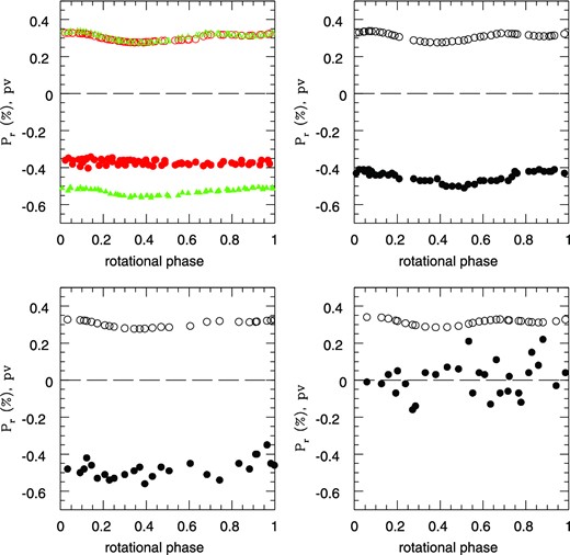
The ‘polarimetric light curves’ used in the present analysis, namely the plots of Pr versus the computed rotational phase at each epoch of measurement (full symbols). Each plot shows also the average albedo of the region of the Vesta's surface visible at the corresponding epochs of observation, plotted against the corresponding rotational phase (open symbols). The albedo values show a sinusoidal variation around a value of about 0.30. Top-left: 1977 (red) and 1978 (green) data. Top-right: 1986 data. bottom-left: 1988 data. Bottom-right: 2011 data. Note that we plot the Pr parameter, namely the fraction of linear polarization with sign, and that nearly all the measurement were taken at phase angles corresponding to negative polarization. The general trend is an increasing of polarization for decreasing albedo, apart from the noisy 2011 data, which were taken close to the inversion angle, when the degree of polarization was close to zero.
All the polarimetric light curves considered in our work are given in Table A1 in the appendix, and they are shown in Fig. 3, together with the corresponding average albedo of the surface of Vesta visible at the epoch of each single measurement, derived as described in the following section.
5 Linking remote observations to local regions of Vesta's surface
The first part of the work consisted of a computation of the coordinates of the sub-Earth point on the surface of Vesta, corresponding to the epoch of each available observation. For this computation, we used spice routines and kernels with information like the sidereal rotation period and the orientation of the spin axis updated after the Dawn measurement. We can therefore compute with satisfactory accuracy the position of the sub-Earth point even for epochs corresponding to the oldest observations in our sample. Observing Vesta over times of the order of one rotational cycle means that the sub-Earth point remains practically constant in latitude, whereas the longitude varies as the time passes. For the computation, we used the Claudia prime meridian reference system (Russell et al. 2012).
Dawn data include a huge amount of information. In this paper we focus our attention on data of the local topography, albedo, and height with respect to the average best-fitting ellipsoid shape of Vesta. The height is also related to the slope of the terrain, though in a non-straightforward way, in the sense that surface slopes (more or less steep) must be present to produce the extreme values of (positive or negative) height. Knowing the location of the sub-Earth point, namely the intersection of the line of sight from the observer with Vesta's surface, we know the hemisphere of Vesta that was visible at the epoch of each measurement. This is shown in Fig. 4. In this figure, for each available polarization light curve, we plot, superimposed to the Vesta lithological map already shown in Fig. 1, the coordinates of the sub-Earth point corresponding to each observation epoch (each ‘point’ of each polarization light curve). To retrieve the values, we have first computed for each polarimetric light curve the average value of linear polarization, and we have then assigned a colour code according to the difference between each single measurement and the average value. In this way, we overcome some problems in comparing the behaviour of different curves, since each one was obtained at a different phase angle, and exhibits, correspondingly, a different value of average polarization. In the plots, increasingly darker colours are used to indicate increasing absolute values of linear polarization, and lighter colours correspond to decreasing absolute values of polarization. The whole interval of variation is generally of the order of 4–5 per cent, with the only one exception of the noisy 2011 data, as shown in Fig. 3. It is easy to see that the 1977 and 1988 data were obtained with the sub-Earth point located at very similar latitude (around 20°) in the Northern hemisphere. Among them, the 1977 data do not exhibit a clear trend of variation against longitude, as we already saw in Fig. 3. The best-quality data are those of 1978 and 1986 data, which were obtained at similar values of latitude of the sub-Earth point, at about −10° in the Southern hemisphere. The 2011 data correspond to a larger negative latitude of about −22°. As mentioned above, these observations were carried out at a phase angle close to the inversion angle, where the degree of polarization drops to zero. It is therefore not surprising that the 2011 data do not display any significant trend.
The compositional map of Vesta shown in Fig. 1, with superimposed locations of the sub-Earth points at the epochs of the polarimetric light curves at our disposal. Different symbol shapes are used for different polarimetric light curves. For each curve, which runs along Vesta parallels, different values of linear polarization with respect to the average value for each curve, are indicated by using a scale of colours (from white for lowest polarization, to deep red for highest polarization, see text). The horizontal strips of data represent, from north to south (top to bottom) the 1988, 1977, 1978, 1986, 2011 polarimetric light curves, respectively.
In Fig. 5, we repeat this exercise, but we plot the averages of all available polarimetric data corresponding to sub-Earth points found in different intervals (30° in width) of longitude on Vesta. In this way, we want to better display the general trend of polarization versus longitude. More precisely, for each point belonging to each polarimetric light curve, we plot the difference of measured polarization with respect to the average value of its curve. In each interval of longitudes we make a weighted average of these values. The weights were chosen according to the average value of polarization of each light curve, because in this way we weight more the polarimetric light curves for which the average polarization is stronger (making it easier to detect any modulation of polarization). This choice has also the advantage to assign nearly zero statistical weight to the very noisy 2011 data, obtained when the average polarization was close to zero. Moreover, a low weight is also assigned to the low-quality 1977 data, which exhibit a lower degree of polarization with respect to the 1978 and 1986 curves, the best data at our disposal as already discussed above. In the figure, the resulting points are plotted at zero latitude, which is approximately the average value of the latitude of the sub-Earth point in our data set. As in the previous figure, we indicate by means of lighter colour the measurements for which the polarization was lower than the average, whereas we use darker colours in the opposite case. As for the size of the circles, we used an angular radius of 30°, corresponding to the adopted intervals of local longitude.
The same as Fig. 4, but here we plot the weighted averages of all the differences of polarization with respect to the average value of each curve, and we plot all data belonging to different intervals of longitude having a width of 30° (see text).
Note that in this and the following figures in this section we plot the absolute value of Pr, which corresponds to the measured fraction of linear polarization. In all cases but a few 2011 data, the measurements were obtained in the branch of negative polarization.
The purpose of our analysis is to see whether the disc-integrated degree of linear polarization of Vesta is systematically higher or lower depending on the area visible at different epochs. Looking at Figs 4 and 5, we confirm an overall variation of linear polarization having a roughly sinusoidal variation over 360° of longitude. It is clear that, even taking into account all necessary caveats due to the noise affecting the measurements, there is a wide region, covering approximately 180° in longitude, and extending between 80° W and about 260° W (or slightly less) in the Northern hemisphere, in which the fraction of linear polarization tends to be higher than average. This region includes a large area of Vesta where the eucrite mineral is found to be most dominant (see Fig. 1).
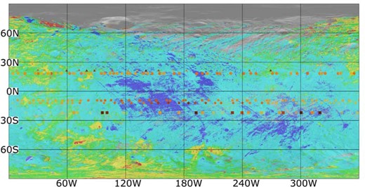
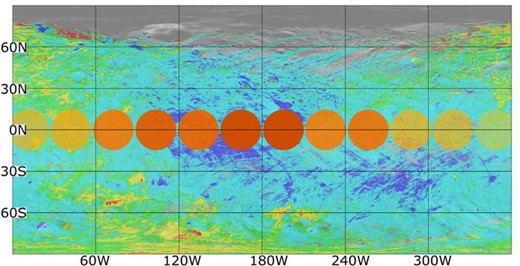
Due to the fact that the fraction of linear polarization of scattered light is known to be strictly linked to albedo, it is interesting to interpret our Vesta data in terms of surface albedo, based on the evidence obtained by Dawn measurements. This is done in Fig. 6, in which the polarimetric data are plotted as in Fig. 4, but using as the background the Dawn albedo map of Vesta. We note that the Dawn albedo values used in our analysis have been obtained using clear filter data, the quantum efficiency of the CCD having its maximum at a wavelength around 0.7 μm (Schroeder et al. 2013), whereas all the ground-based polarimetric data we use were obtained in the Johnson V-band (0.55 μm). This is not important for the main purposes of our analysis, because the differences in the linear polarization in this small wavelength interval are generally very small (Belskaya et al. 2009; Bagnulo, Cellino & Sterzik 2015). Some limited noise may arise, however, when we will combine Dawn and ground-based albedo values obtained from V-band polarimetry in Section 6.

As discussed in previous sections, the surface of Vesta is clearly not homogeneous in albedo. This is easily visible by looking at Fig. 6, where a large, darker than average region is apparent and covers a zone which is found to largely correspond to higher than average polarization values, as already seen in Fig. 4.
Since ground-based observations were disc-integrated, we are led to compute the average value of the albedo in the portion of the surface seen by the observers at each epoch of observation. Using Dawn data, we computed the average value of albedo over areas included in increasingly larger circles centred on the sub-Earth points of all polarimetric measurements. We considered circles having angular radii of 20°, 40° and 60°, respectively, and we realized that in all cases there is a quick convergence of the resulting value of average albedo as the radius of the considered area increases, from the lower to the highest value of considered radius. Typical values in all circumstances differ by no more than 0.015 in average albedo going from the narrowest to the widest considered area. This convinced us that it is not necessary to consider larger areas around the sub-Earth point, what is useful from the point of view of necessary computing time. We used therefore the average albedo values obtained over angular radii of 60° from the sub-Earth points. The effect due to the terminator, that one should in principle take into account when considering larger angular radii, around 90°, also tends to be negligible and hence was disregarded. We are aware that our approach is very simple, but we are confident that the results that we obtain are reliable, since the contribution of zones increasingly far from the sub-Earth point tend to become increasingly weaker in disc-integrated data (the projection varying as the cosine of the angle between the normal to the surface and the direction to the observer). Looking at Fig. 6, and at Fig. 7, where we plot the averaged values of polarization in intervals of longitude 30° wide, as already done in Fig. 5, it is apparent that the highest values of linear polarization tend to be reached when the sub-Earth point was preferentially located close to the large region of low albedo on the Vesta's surface. This trend tends to be sharper for the series of observations carried out in 1978, 1986 and 1988, corresponding to different latitudes of the sub-Earth point. In Fig. 10, we show an albedo–polarization plot based on all the recorded points of our best polarimetric light curves, namely those of 1978 and 1986. A general trend of increasing polarization for decreasing albedo can be clearly seen. This behaviour is in agreement with the known relation (Umov law), between albedo and linear polarization, the latter being generally higher for light scattered by darker surfaces. In this respect, the data displayed in Fig. 10 nicely confirm that Vesta generally obeys the Umov law. If we consider only the best data at our disposal, those of 1978 obtained at phase angles of 11|$_{.}^{\circ}$|1 and 11|$_{.}^{\circ}$|6, we derive the following relation between the degree of linear polarization Pr and geometric albedo pV: |Pr| = (−0.790 ± 0.177) pV + (0.773 ± 0.003). The 1986 data, obtained at slightly different phase angle (13|$_{.}^{\circ}$|2), give similar values for the coefficients, but with much larger error bars.

By looking at Figs 6 and 7, however, we see that there are deviations from a purely albedo-dependent trend, with relatively large absolute values of polarization corresponding also to data obtained when the sub-Earth points were slightly W of the low-albedo region, mainly in the case of polarimetric light curves obtained when the sub-Earth points were located at the highest values of N latitude.
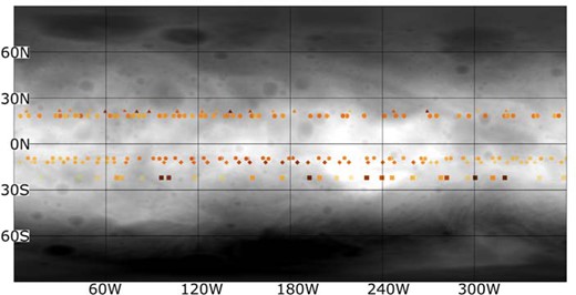
To have a deeper understanding of the situation, it is useful to consider also other Vesta surface data obtained by Dawn. One of the features to be taken into account is the elevation of the surface, which varies in different regions, being generally higher on equatorial regions. If one looks at Figs 8 and 9, where individual and average values of polarization are plotted against the background of an elevation map of Vesta, it is possible to see that relatively high values of polarization seem to be obtained also when the sub-Earth points were located above the region of highest elevation. This region appears as the brightest area in Figs 8 and 9. In general terms, the regions immediately surrounding locations of maximum height above (or below) the average level, must have terrain slopes needed to reach the extreme values of elevation, although it is clear that there is a large variety of possible slope trends. It is also reasonable to suppose that the regions at highest elevations should be covered by thinner-than-average layers of regolith, whereas the deepest regions could be expected to host the deepest layers of regolith. Both local slope and regolith depth can influence the state of polarization. We also note that in the region located just south of the area of highest elevation close to the equator, there is another zone, running SE–NW, in which the eucrite mineral tends again to dominate the surface composition (see Fig. 1). This is interesting, because the larger Eastern region of low average albedo in the Northern hemisphere, where the polarization is found to be high, also corresponds to a region of the surface where the spectroscopic signature of eucrite tends to be predominant (as seen in Fig. 1). It is difficult to say whether this link between high polarization and eucritic composition is directly related to the material composition itself, or to other properties as local surface slope, size of the regolith grains, depth of the regolith. In Fig. 11, we focus on the two best polarization light curves that we have at our disposal, those obtained in 1978 and in 1986, and for each point of them, we plot and compare the longitude–polarization, longitude–average albedo and longitude–average tangential component of gravity, where ‘average’ means that we made, as before, an average of the values found in a region within a circle having a radius of 60° surrounding each sub-Earth point. We computed the tangential component of gravity by using a detailed representation of the shape of Vesta derived from Dawn data (Gaskell 2012), approximated by a grid of triangular facets having sizes of about 700 m. The tangential component for each triangular facet was computed by knowing the distribution of mass in the interior of Vesta, taken from Ermakov et al. (2014), and by making for each triangular facet a numerical computation of the tangential component of the gravitational force, by using a large number (about 80 000) of points uniformly distributed in core, mantle and crust. The resulting value found for each facet was then averaged over all the facets included in the area surrounding each sub-Earth point. This gives an approximation of the average slope of the terrain in each area considered. Though not being a rigorous computation of the local terrain slope, this is a reasonable approximation useful for statistical purposes. Let us refer to this parameter in what follows, for sake of simplicity, as the ‘gravitational slope’. In principle, a steep slope should correspond to zones where surface regolith may be expected to be relatively not very deep (since it tends to move down following the slope).

Because the 1978 and 1986 curves were obtained at very similar values of the latitude of the sub-Earth point, it is not surprising that the trends of the plots shown in Fig. 11 tend to be very similar for the 1978 and 1986 data. The difference in the degree of linear polarization are due to the difference in phase angle characterizing the two data sets. If we look at Fig. 11, and we compare the morphology of the curves shown in each of the three plots, we can see some interesting facts. First, the longitude–albedo and longitude–polarization plots appear to be anticorrelated, as expected, as shown in Fig. 10, but this anticorrelation is not seen everywhere. In particular, a secondary drop of the albedo starting around 250° in longitude, seems not to have any influence on polarization, particularly in the case of the 1978 polarization light curve. The 1986 data also show a decrease of the degree of linear polarization at longitudes beyond 250°, in spite of the fact that albedo is also decreasing. Note that the behaviour of polarization in this limited range of longitudes corresponds to a region of Fig. 10, between about 0.31 and 0.325 in albedo, where the polarization–albedo data are apparently more scattered. Secondly, the polarization seems to show an overall correlation with the behaviour of the gravitational slope. This correlation seems to be sharper in the case of the 1986 curve, since it extends up to the longitudes where the gravitational slope tends to raise again, after reaching a minimum around 315° in longitude. At longitudes larger than about 250°, it seems that the correlation of polarization with gravitational slope is stronger than the anticorrelation with the albedo. We note that both albedo and compositional variations with longitude are essentially identical between the 1978 and 1986 data sets. Therefore, more traditional explanations for polarization variability cannot be invoked to explain what we see in Fig. 11 at high longitude values. It is therefore interesting to note that this region is the one reaching the maximum elevation (see Fig. 8). This suggests that the gravitational slope, which is rapidly decreasing beyond 250° in longitude, corresponds to a region of rapid change of the average terrain slope after reaching a maximum of elevation.
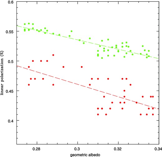
Albedo–linear polarization plot for each point of the 1978 (green) and 1986 (red) polarization curves. The corresponding linear best-fitting solutions are also shown for each curve.
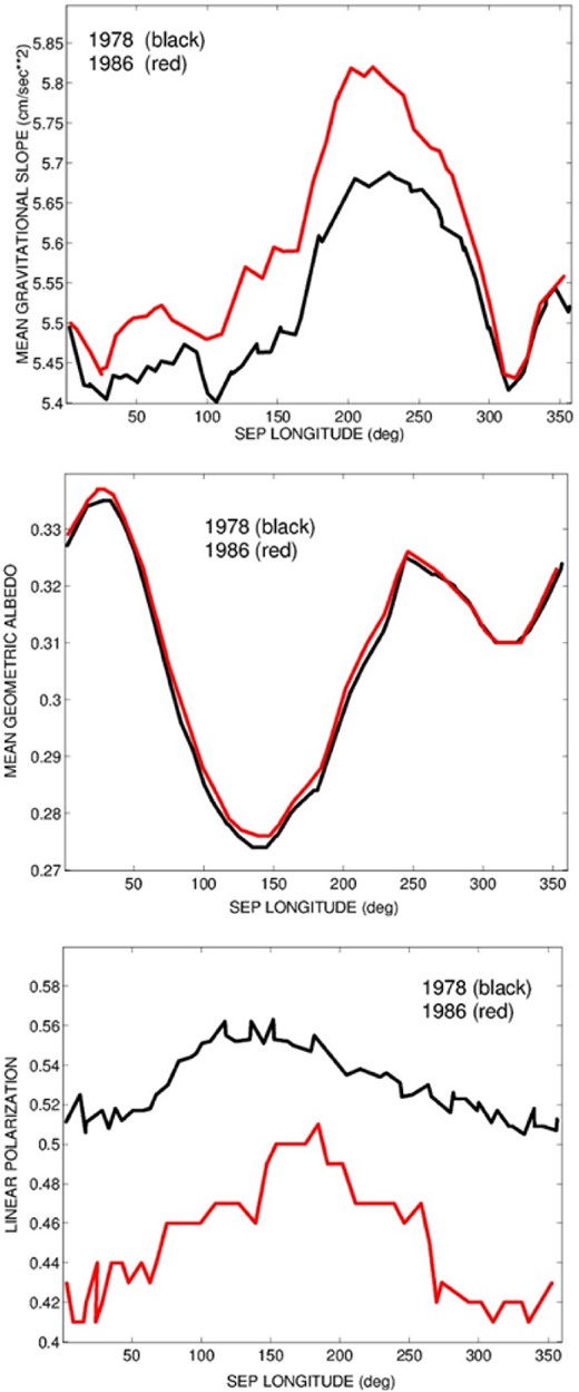
From top to bottom: average tangential gravity component (see text), average albedo and measured linear polarization, respectively, plotted against Vesta longitude, for each point of the 1978 (black) and 1986 (red) polarization curves.
Summarizing, it seems that the data at our disposal generally confirm the well-known link between albedo and polarization. At the same time, the situation seems to be more complicated, with other surface properties, including elevation and surface slope, playing some important role. It is also important to note that, in terms of composition, the highest values of polarization tend to be reached when the sub-Earth point is located in regions characterized by the strongest spectral features of eucritic material. These regions tend to coincide, but not completely, with the regions of lowest albedo.
6 TOWARDS A NEW ASSESSMENT OF THE SLOPE–ALBEDO RELATION
Having polarization measurements corresponding to observations of regions of Vesta having different values of average albedo, allows us to perform several interesting exercises. In particular, we can regroup our data by subdividing them in different subsamples corresponding to observations of areas of different albedo. These subsamples merge together data belonging to the different polarimetric light curves at our disposal, which were obtained at different values of phase angle. The phase angle coverage is suitable for the derivation of the polarization slope (see Section 3). We can produce a number of different phase–polarization curves corresponding to polarimetric measurements of regions of the surface for which we know a priori the albedo. The purpose of this exercise is therefore to test whether we can confirm some well-known general results of asteroid polarimetry, namely and foremost the relation between the geometric albedo pV and the polarimetric slope.
In our analysis, we split our data into four albedo classes: pV < 0.29, 0.29 ≤ pV < 0.31, 0.31 ≤ pV < 0.33, and pV > 0.33, respectively. The resulting phase–polarization curves are shown in Fig. 12. In this figure, we plot also the best-fitting linear representations obtained by a least-squares procedure in which we used only data obtained at phase angles above 13°, where the overall trend of the phase–polarization curves is linear. In computing these linear fits, we used average values for all data obtained at the same value of phase angle (within 0|$_{.}^{\circ}$|1). This is important, because this tends to mitigate the problem posed by our 2011 data, obtained close to the polarization inversion angle, which are very noisy, and vary up and down in an apparently random way around zero polarization. These 2011 data are important to build the polarimetric slopes, and our averaging procedure makes our results less dependent on their intrinsic noise.
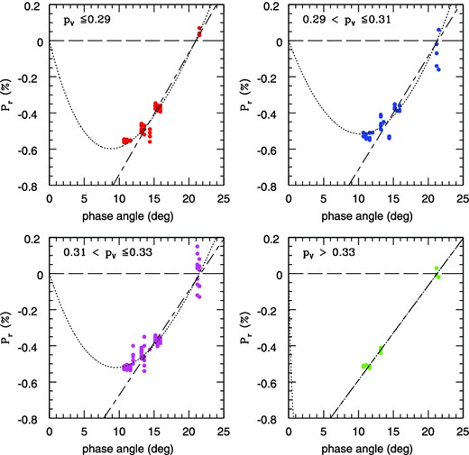
Phase–polarization curves of Vesta corresponding to the different values of average albedo of the visible regions visible at the epochs of different polarization measurements. The dotted curve represent for each phase–polarization curve a best fit of the data using the relation Pr = A(e−α/B − 1) + C · α, where α is the phase angle. We also plot for each case the linear fit obtained considering only the observations obtained at phase angles ≥13°.
In Fig. 12, we show also a general best fit of the data for each albedo class, using the exponential–linear relation mentioned in Section 3, and applied to all data points available in each albedo class, with no smoothing or phase limits. As can be seen, our data, though covering only a limited interval of phase angles, are still sufficient to derive a decent representation of the general variation of polarization as a function of phase angle.
In principle, we expect to obtain steeper polarimetric slopes when considering data corresponding to darker regions of Vesta. Even beyond expectations, considering the non-ideal quality of many of our data, the results very nicely confirm the predictions, as shown in Table 1, in which we list for each of our four subsamples, the average albedo of the regions of Vesta associated with the different polarimetric measurements, the resulting polarimetric slope h, and also the value of the inversion angle αinv found from the linear best fit of the data.
Average albedo, polarimetric slope and inversion angle for each of the four data subsamples considered in our analysis.
| pV | h | αinv |
|---|---|---|
| 0.282 ± 0.014 | 0.0669 ± 0.0087 | 21.1 |
| 0.301 ± 0.019 | 0.0622 ± 0.0122 | 21.4 |
| 0.320 ± 0.018 | 0.0571 ± 0.0141 | 22.0 |
| 0.335 ± 0.007 | 0.0514 ± 0.0153 | 21.6 |
| pV | h | αinv |
|---|---|---|
| 0.282 ± 0.014 | 0.0669 ± 0.0087 | 21.1 |
| 0.301 ± 0.019 | 0.0622 ± 0.0122 | 21.4 |
| 0.320 ± 0.018 | 0.0571 ± 0.0141 | 22.0 |
| 0.335 ± 0.007 | 0.0514 ± 0.0153 | 21.6 |
In Fig. 13, we show the resulting best fit of the slope–albedo law (equation 1) using our Vesta data (black dots). In the same figure, we also show, using green symbols, the slope–polarization data recently used by Cellino et al. (2015) to derive an updated best fit of the slope–albedo relation. These data correspond to objects belonging to a list published by Shevchenko & Tedesco (2006), which includes asteroids for which we have extremely accurate determination of the size and good knowledge of the absolute magnitude, from which it is possible to derive correspondingly reliable values of the geometric albedo. In particular, Cellino et al. (2015) computed two distinct linear best fits of available data: one using all the objects of the Shevchenko & Tedesco (2006) sample for which we have accurate polarimetric slopes, and another limiting the analysis to all and only the calibration asteroids having geometric albedo larger than 0.08. The reason is that it has long been known that the slope–albedo relation tends to saturate at low albedo, and this fact was confirmed by the results of the Cellino et al. (2015) analysis. In Fig. 13, we plot (in green) only the linear best fit (in log–log scale) resulting from excluding low-albedo objects. These objects (four asteroids, having albedo <0.08) are plotted in the figure, but they were not used in the computation of the linear best fit.
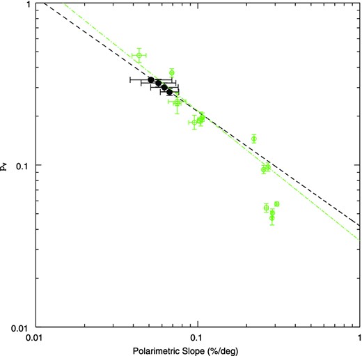
The new derived values of geometric albedo versus polarimetric slope resulting from our analysis of Vesta data (black symbols) plotted together with the slope–polarization data calibration recently derived by Cellino et al. (2015, green symbols). Limiting our analysis to our Vesta data we derive a linear best fit of the slope–albedo law, represented as the black, dashed line. This new calibration is in good agreement with the recent calibration of the slope–albedo relation obtained by Cellino et al. (2015) for asteroids having albedo larger than 0.08 (green, dash–dotted line).
We can make two comments: first, it is remarkable how the four Vesta data tend to be well aligned in the expected way, i.e. with increasing polarimetric slope for decreasing albedo. Secondly, the linear best fit of the four Vesta points, shown in black in Fig. 13, nicely agrees with the general calibration of the slope–albedo relation found by Cellino et al. (2015) using a larger data set of asteroids having moderate or high albedo. Adding the new Vesta data to the full data set would tend to slightly decrease the slope of the linear best fit. This is interesting, because a steep slope–albedo relation would lead to predict high, and, possibly in some cases, exceedingly high, values of albedo for asteroids displaying shallow polarimetric slopes, as noted by Cellino et al. (2015).
7 CONCLUSIONS
We have analysed all available polarimetric light curves of the asteroid (4) Vesta. By computing the regions of the surface that were visible at the epochs of each polarimetric measurement, according to the detailed analysis of Vesta's surface performed by the Dawn mission, we obtain for the first time a link between disc-integrated polarimetric measurements and the local properties of the visible surface of an asteroid. We confirm the relation between albedo and polarization, which gives rise in the case of Vesta to a sinusoidal variation of polarization, due to a region of low albedo covering about 180° deg in longitude. We find, however, that albedo alone may be not sufficient to completely justify the observed polarimetric behaviour. Some effect due to surface slope and/or mineralogical composition is suggested by the polarimetric data, although this deserves confirmation that can hopefully come in the future by new, high-quality observations.
The single polarimetric measurements belonging to different polarimetric light curves can be analysed by splitting them into subsets corresponding to observations of regions of Vesta's surface characterized by different average albedo values. By doing so, we were able to compute four distinct polarimetric slopes, which nicely fit the traditional form of the slope–albedo relation given by equation (1). These values suggest a modification of the linear best fit obtained using currently available data for calibration asteroids of different albedo. In particular, Vesta data are in excellent agreement with the slope–albedo relation that is obtained by excluding from the analysis asteroids having albedos lower than about 0.08.
We thank the Referee, S. Wiktorowicz, for his careful review, that led to a substantial improvement of this work. This project was funded by the Italian INAF, in the framework of the programme PRIN-INAF 2011. RGH gratefully acknowledges financial support by CONICET through PIP 114-201101-00358.
The phase angle is the angle between the directions to the sun and to the observer, as seen from the object.
REFERENCES
APPENDIX A
The polarimetric light curves adopted in this work. Each line refers to one single measurement. The columns give the latitude and longitude of the sub-Earth point at the epoch of observation, the value of Pr, the average albedo of the visible hemisphere, the phase angle α and the year of observation, respectively.
| LatSE | LongSE | Pr | 〈pV〉 | α | Year |
|---|---|---|---|---|---|
| (deg) | (deg) | (per cent) | (deg) | ||
| 18.4 | 139.7 | −0.370 | 0.277 | 15.2 | 1977 |
| 18.4 | 112.6 | −0.360 | 0.278 | 15.2 | 1977 |
| 18.4 | 100.2 | −0.361 | 0.284 | 15.2 | 1977 |
| 18.4 | 80.0 | −0.352 | 0.293 | 15.2 | 1977 |
| 18.4 | 42.9 | −0.355 | 0.322 | 15.2 | 1977 |
| 18.4 | 351.3 | −0.379 | 0.323 | 15.2 | 1977 |
| 18.4 | 337.6 | −0.360 | 0.318 | 15.2 | 1977 |
| 18.4 | 322.2 | −0.373 | 0.314 | 15.2 | 1977 |
| 18.4 | 304.5 | −0.379 | 0.313 | 15.2 | 1977 |
| 18.4 | 273.2 | −0.368 | 0.318 | 15.2 | 1977 |
| 18.4 | 247.3 | −0.376 | 0.316 | 15.2 | 1977 |
| 18.4 | 227.1 | −0.370 | 0.295 | 15.2 | 1977 |
| 18.4 | 213.6 | −0.378 | 0.291 | 15.2 | 1977 |
| 18.4 | 198.4 | −0.378 | 0.289 | 15.2 | 1977 |
| 18.4 | 175.2 | −0.361 | 0.285 | 15.2 | 1977 |
| 18.4 | 160.0 | −0.357 | 0.283 | 15.2 | 1977 |
| 18.3 | 143.5 | −0.358 | 0.278 | 15.2 | 1977 |
| 18.3 | 122.9 | −0.362 | 0.277 | 15.2 | 1977 |
| 18.3 | 105.7 | −0.360 | 0.281 | 15.2 | 1977 |
| 18.3 | 86.8 | −0.346 | 0.290 | 15.2 | 1977 |
| 18.3 | 68.4 | −0.354 | 0.301 | 15.2 | 1977 |
| 18.3 | 50.8 | −0.342 | 0.317 | 15.2 | 1977 |
| 18.3 | 44.2 | −0.349 | 0.321 | 15.2 | 1977 |
| 18.3 | 30.5 | −0.356 | 0.326 | 15.2 | 1977 |
| 18.3 | 13.2 | −0.348 | 0.327 | 15.2 | 1977 |
| 18.3 | 175.4 | −0.376 | 0.285 | 15.5 | 1977 |
| 18.3 | 158.1 | −0.359 | 0.282 | 15.5 | 1977 |
| 18.3 | 140.1 | −0.368 | 0.277 | 15.5 | 1977 |
| 18.3 | 125.7 | −0.381 | 0.277 | 15.5 | 1977 |
| 18.3 | 109.1 | −0.387 | 0.279 | 15.5 | 1977 |
| 18.3 | 96.7 | −0.386 | 0.285 | 15.5 | 1977 |
| 18.3 | 76.7 | −0.388 | 0.296 | 15.5 | 1977 |
| 18.3 | 64.9 | −0.388 | 0.304 | 15.5 | 1977 |
| 18.3 | 46.3 | −0.403 | 0.320 | 15.5 | 1977 |
| 18.3 | 33.2 | −0.394 | 0.325 | 15.5 | 1977 |
| 18.3 | 20.1 | −0.381 | 0.327 | 15.5 | 1977 |
| 18.3 | 318.7 | −0.374 | 0.313 | 15.5 | 1977 |
| 18.3 | 304.2 | −0.360 | 0.313 | 15.5 | 1977 |
| 18.3 | 287.7 | −0.374 | 0.318 | 15.5 | 1977 |
| 18.3 | 273.9 | −0.367 | 0.318 | 15.5 | 1977 |
| 18.2 | 203.2 | −0.374 | 0.290 | 15.9 | 1977 |
| 18.2 | 170.0 | −0.388 | 0.285 | 15.9 | 1977 |
| 18.2 | 155.4 | −0.393 | 0.281 | 15.9 | 1977 |
| 18.2 | 138.4 | −0.382 | 0.277 | 15.9 | 1977 |
| 18.2 | 124.1 | −0.369 | 0.277 | 15.9 | 1977 |
| 18.2 | 106.1 | −0.379 | 0.280 | 15.9 | 1977 |
| 18.2 | 87.0 | −0.368 | 0.290 | 15.9 | 1977 |
| 18.2 | 56.9 | −0.357 | 0.311 | 15.9 | 1977 |
| 18.2 | 36.3 | −0.353 | 0.324 | 15.9 | 1977 |
| 18.2 | 20.4 | −0.361 | 0.327 | 15.9 | 1977 |
| 18.2 | 8.0 | −0.360 | 0.327 | 15.9 | 1977 |
| 18.2 | 348.7 | −0.360 | 0.321 | 15.9 | 1977 |
| 18.2 | 335.2 | −0.385 | 0.317 | 15.9 | 1977 |
| 18.2 | 316.6 | −0.384 | 0.313 | 15.9 | 1977 |
| 18.2 | 293.9 | −0.382 | 0.317 | 15.9 | 1977 |
| 18.2 | 269.1 | −0.384 | 0.318 | 15.9 | 1977 |
| 18.2 | 252.6 | −0.386 | 0.318 | 15.9 | 1977 |
| 18.2 | 240.1 | −0.390 | 0.310 | 15.9 | 1977 |
| 18.2 | 216.1 | −0.384 | 0.292 | 15.9 | 1977 |
| 18.2 | 203.8 | −0.379 | 0.290 | 15.9 | 1977 |
| 18.2 | 192.7 | −0.386 | 0.287 | 15.9 | 1977 |
| 18.2 | 147.9 | −0.385 | 0.279 | 15.9 | 1977 |
| 18.2 | 131.1 | −0.366 | 0.277 | 15.9 | 1977 |
| 18.2 | 117.4 | −0.359 | 0.277 | 15.9 | 1977 |
| 18.2 | 97.9 | −0.377 | 0.285 | 15.9 | 1977 |
| 18.2 | 83.7 | −0.357 | 0.291 | 15.9 | 1977 |
| 18.2 | 69.9 | −0.361 | 0.300 | 15.9 | 1977 |
| 18.2 | 37.4 | −0.372 | 0.324 | 15.9 | 1977 |
| −9.4 | 166.1 | −0.550 | 0.281 | 10.7 | 1978 |
| −9.4 | 151.9 | −0.563 | 0.276 | 10.7 | 1978 |
| −9.4 | 135.1 | −0.553 | 0.274 | 10.7 | 1978 |
| −9.4 | 117.1 | −0.562 | 0.278 | 10.7 | 1978 |
| −9.4 | 96.5 | −0.546 | 0.288 | 10.7 | 1978 |
| −9.4 | 76.0 | −0.530 | 0.303 | 10.7 | 1978 |
| −9.4 | 57.8 | −0.517 | 0.320 | 10.7 | 1978 |
| −9.4 | 38.2 | −0.518 | 0.333 | 10.7 | 1978 |
| −9.4 | 16.9 | −0.511 | 0.334 | 10.7 | 1978 |
| −9.4 | −3.4 | −0.513 | 0.324 | 10.7 | 1978 |
| −9.3 | −20.0 | −0.518 | 0.315 | 10.7 | 1978 |
| −9.3 | −38.2 | −0.509 | 0.310 | 10.7 | 1978 |
| −9.3 | −60.0 | −0.521 | 0.313 | 10.7 | 1978 |
| −9.3 | −80.4 | −0.516 | 0.320 | 10.7 | 1978 |
| −9.3 | −94.0 | −0.524 | 0.322 | 10.7 | 1978 |
| −9.3 | −116.6 | −0.531 | 0.324 | 10.7 | 1978 |
| −9.2 | 92.6 | −0.544 | 0.291 | 11.1 | 1978 |
| −9.2 | 67.5 | −0.525 | 0.311 | 11.1 | 1978 |
| −9.2 | 50.8 | −0.517 | 0.326 | 11.1 | 1978 |
| −9.2 | 33.4 | −0.508 | 0.335 | 11.1 | 1978 |
| −9.2 | 16.7 | −0.506 | 0.334 | 11.1 | 1978 |
| −9.2 | 2.4 | −0.511 | 0.327 | 11.1 | 1978 |
| −9.2 | −13.5 | −0.509 | 0.318 | 11.1 | 1978 |
| −9.2 | −27.1 | −0.505 | 0.312 | 11.1 | 1978 |
| −9.2 | −46.6 | −0.517 | 0.310 | 11.1 | 1978 |
| −9.2 | −61.0 | −0.517 | 0.313 | 11.1 | 1978 |
| −9.2 | −77.6 | −0.523 | 0.319 | 11.1 | 1978 |
| −9.2 | −96.4 | −0.530 | 0.322 | 11.1 | 1978 |
| −9.2 | −115.4 | −0.524 | 0.325 | 11.1 | 1978 |
| −9.2 | −131.1 | −0.534 | 0.312 | 11.1 | 1978 |
| −9.2 | −155.3 | −0.535 | 0.301 | 11.1 | 1978 |
| −9.2 | 179.1 | −0.547 | 0.284 | 11.1 | 1978 |
| −9.2 | 152.7 | −0.553 | 0.276 | 11.1 | 1978 |
| −9.2 | 136.1 | −0.562 | 0.274 | 11.1 | 1978 |
| −9.2 | 117.9 | −0.555 | 0.278 | 11.1 | 1978 |
| −9.2 | 100.5 | −0.551 | 0.285 | 11.1 | 1978 |
| −9.2 | 83.8 | −0.542 | 0.296 | 11.1 | 1978 |
| −9.0 | −78.3 | −0.526 | 0.319 | 11.6 | 1978 |
| −9.0 | −107.8 | −0.525 | 0.324 | 11.6 | 1978 |
| −9.0 | −126.6 | −0.536 | 0.315 | 11.6 | 1978 |
| −9.0 | −145.4 | −0.538 | 0.306 | 11.6 | 1978 |
| −9.0 | −162.0 | −0.550 | 0.297 | 11.6 | 1978 |
| −9.0 | −178.5 | −0.555 | 0.284 | 11.6 | 1978 |
| −9.0 | 162.5 | −0.552 | 0.280 | 11.6 | 1978 |
| −9.0 | 145.1 | −0.551 | 0.274 | 11.6 | 1978 |
| −9.0 | 124.7 | −0.552 | 0.276 | 11.6 | 1978 |
| −9.0 | 106.6 | −0.552 | 0.282 | 11.6 | 1978 |
| −9.0 | 63.3 | −0.518 | 0.315 | 11.6 | 1978 |
| −9.0 | 42.8 | −0.512 | 0.331 | 11.6 | 1978 |
| −9.0 | 28.6 | −0.517 | 0.335 | 11.6 | 1978 |
| −9.0 | 12.7 | −0.525 | 0.332 | 11.6 | 1978 |
| −9.0 | −4.1 | −0.507 | 0.323 | 11.6 | 1978 |
| −9.0 | −19.9 | −0.509 | 0.315 | 11.6 | 1978 |
| −9.0 | −35.7 | −0.509 | 0.310 | 11.6 | 1978 |
| −9.0 | −50.8 | −0.511 | 0.310 | 11.6 | 1978 |
| −9.0 | −69.6 | −0.523 | 0.317 | 11.6 | 1978 |
| −9.0 | −93.8 | −0.524 | 0.322 | 11.6 | 1978 |
| −11.8 | 25.2 | −0.440 | 0.337 | 13.2 | 1986 |
| −11.8 | 17.2 | −0.420 | 0.335 | 13.2 | 1986 |
| −11.8 | 3.0 | −0.430 | 0.329 | 13.2 | 1986 |
| −11.8 | −7.1 | −0.430 | 0.323 | 13.2 | 1986 |
| −11.8 | −29.0 | −0.420 | 0.312 | 13.2 | 1986 |
| −11.8 | −24.0 | −0.410 | 0.314 | 13.2 | 1986 |
| −11.8 | −32.7 | −0.420 | 0.310 | 13.2 | 1986 |
| −11.8 | −41.5 | −0.420 | 0.310 | 13.2 | 1986 |
| −11.8 | −49.6 | −0.410 | 0.310 | 13.2 | 1986 |
| −11.8 | −58.3 | −0.420 | 0.312 | 13.2 | 1986 |
| −11.8 | −67.1 | −0.420 | 0.316 | 13.2 | 1986 |
| −11.8 | −90.3 | −0.420 | 0.322 | 13.2 | 1986 |
| −11.8 | −86.6 | −0.430 | 0.321 | 13.2 | 1986 |
| −11.8 | −95.4 | −0.450 | 0.323 | 13.2 | 1986 |
| −11.8 | −101.5 | −0.470 | 0.324 | 13.2 | 1986 |
| −11.8 | −113.6 | −0.460 | 0.326 | 13.2 | 1986 |
| −11.8 | −121.0 | −0.470 | 0.322 | 13.2 | 1986 |
| −11.8 | −130.4 | −0.470 | 0.315 | 13.2 | 1986 |
| −11.8 | −142.6 | −0.470 | 0.310 | 13.2 | 1986 |
| −11.8 | −148.6 | −0.470 | 0.307 | 13.2 | 1986 |
| −11.8 | −158.1 | −0.490 | 0.302 | 13.2 | 1986 |
| −11.8 | −168.9 | −0.490 | 0.293 | 13.2 | 1986 |
| −11.8 | −175.6 | −0.510 | 0.288 | 13.2 | 1986 |
| −11.8 | 175.0 | −0.500 | 0.285 | 13.2 | 1986 |
| −11.8 | 164.2 | −0.500 | 0.282 | 13.2 | 1986 |
| −11.8 | 154.1 | −0.500 | 0.278 | 13.2 | 1986 |
| −11.8 | 147.3 | −0.490 | 0.276 | 13.2 | 1986 |
| −11.8 | 139.2 | −0.460 | 0.276 | 13.2 | 1986 |
| −11.8 | 127.1 | −0.470 | 0.277 | 13.2 | 1986 |
| −11.8 | 118.3 | −0.470 | 0.279 | 13.2 | 1986 |
| −11.8 | 110.3 | −0.470 | 0.283 | 13.2 | 1986 |
| −11.8 | 99.5 | −0.460 | 0.288 | 13.2 | 1986 |
| −11.8 | 75.2 | −0.460 | 0.306 | 13.2 | 1986 |
| −11.8 | 67.8 | −0.440 | 0.313 | 13.2 | 1986 |
| −11.8 | 63.1 | −0.430 | 0.317 | 13.2 | 1986 |
| −11.8 | 57.0 | −0.440 | 0.323 | 13.2 | 1986 |
| −11.8 | 47.6 | −0.430 | 0.329 | 13.2 | 1986 |
| −11.8 | 42.9 | −0.440 | 0.332 | 13.2 | 1986 |
| −11.8 | 35.4 | −0.440 | 0.336 | 13.2 | 1986 |
| −11.8 | 28.7 | −0.420 | 0.337 | 13.2 | 1986 |
| −11.8 | 24.0 | −0.410 | 0.337 | 13.2 | 1986 |
| −11.8 | 15.2 | −0.410 | 0.334 | 13.2 | 1986 |
| −11.8 | 7.8 | −0.410 | 0.331 | 13.2 | 1986 |
| 21.6 | 74.5 | −0.510 | 0.296 | 12.0 | 1988 |
| 21.6 | 52.0 | −0.460 | 0.315 | 12.0 | 1988 |
| 21.6 | 39.6 | −0.480 | 0.322 | 12.0 | 1988 |
| 21.6 | 32.9 | −0.500 | 0.324 | 12.0 | 1988 |
| 21.6 | −6.4 | −0.450 | 0.323 | 12.0 | 1988 |
| 21.6 | −30.0 | −0.400 | 0.316 | 12.0 | 1988 |
| 21.6 | −42.4 | −0.480 | 0.313 | 12.0 | 1988 |
| 21.6 | −60.3 | −0.450 | 0.315 | 12.0 | 1988 |
| 21.3 | −177.5 | −0.490 | 0.285 | 13.6 | 1988 |
| 21.3 | 169.0 | −0.470 | 0.287 | 13.6 | 1988 |
| 21.3 | 154.4 | −0.520 | 0.282 | 13.6 | 1988 |
| 21.3 | 133.1 | −0.470 | 0.277 | 13.6 | 1988 |
| 21.3 | 11.8 | −0.480 | 0.327 | 13.6 | 1988 |
| 21.3 | −0.6 | −0.460 | 0.325 | 13.6 | 1988 |
| 21.3 | −13.0 | −0.350 | 0.321 | 13.6 | 1988 |
| 21.3 | −32.0 | −0.400 | 0.315 | 13.6 | 1988 |
| 21.3 | −92.7 | −0.540 | 0.319 | 13.6 | 1988 |
| 21.3 | −114.0 | −0.510 | 0.315 | 13.6 | 1988 |
| 21.3 | −142.1 | −0.450 | 0.292 | 13.6 | 1988 |
| 21.2 | 141.6 | −0.560 | 0.278 | 14.4 | 1988 |
| 21.2 | 123.7 | −0.490 | 0.277 | 14.4 | 1988 |
| 21.2 | 107.9 | −0.510 | 0.280 | 14.4 | 1988 |
| 21.2 | 90.0 | −0.530 | 0.288 | 14.4 | 1988 |
| 21.2 | 82.1 | −0.540 | 0.292 | 14.4 | 1988 |
| 21.2 | 61.9 | −0.530 | 0.306 | 14.4 | 1988 |
| 21.2 | 43.9 | −0.420 | 0.320 | 14.4 | 1988 |
| −22.1 | 102.5 | −0.140 | 0.296 | 21.2 | 2011 |
| −22.1 | 85.8 | −0.020 | 0.307 | 21.2 | 2011 |
| −22.1 | 72.5 | 0.050 | 0.319 | 21.2 | 2011 |
| −22.1 | 57.0 | 0.030 | 0.332 | 21.2 | 2011 |
| −22.1 | 20.9 | −0.010 | 0.340 | 21.2 | 2011 |
| −22.1 | −5.4 | 0.040 | 0.327 | 21.2 | 2011 |
| −22.1 | −21.1 | −0.030 | 0.318 | 21.2 | 2011 |
| −22.1 | −43.2 | 0.220 | 0.312 | 21.2 | 2011 |
| −22.1 | −62.0 | 0.150 | 0.313 | 21.2 | 2011 |
| −22.1 | −80.1 | −0.120 | 0.319 | 21.2 | 2011 |
| −22.1 | −102.0 | −0.060 | 0.324 | 21.2 | 2011 |
| −22.1 | −121.6 | 0.110 | 0.327 | 21.2 | 2011 |
| −22.1 | −141.1 | 0.030 | 0.320 | 21.2 | 2011 |
| −22.1 | −161.3 | −0.070 | 0.309 | 21.2 | 2011 |
| −22.1 | −50.9 | 0.080 | 0.311 | 21.5 | 2011 |
| −22.1 | −67.1 | 0.040 | 0.315 | 21.5 | 2011 |
| −22.1 | −84.0 | −0.070 | 0.320 | 21.5 | 2011 |
| −22.1 | −99.8 | 0.020 | 0.323 | 21.5 | 2011 |
| −22.1 | −115.2 | −0.070 | 0.328 | 21.5 | 2011 |
| −22.1 | −131.3 | −0.130 | 0.324 | 21.5 | 2011 |
| −22.1 | −150.5 | 0.040 | 0.316 | 21.5 | 2011 |
| −22.1 | −167.9 | 0.210 | 0.304 | 21.5 | 2011 |
| −22.1 | 174.9 | 0.060 | 0.292 | 21.5 | 2011 |
| −22.1 | 155.8 | 0.070 | 0.286 | 21.5 | 2011 |
| −22.1 | 136.6 | 0.030 | 0.285 | 21.5 | 2011 |
| −22.1 | 119.0 | 0.040 | 0.288 | 21.5 | 2011 |
| −22.1 | 97.7 | −0.160 | 0.299 | 21.5 | 2011 |
| −22.1 | 69.5 | −0.070 | 0.322 | 21.5 | 2011 |
| −22.1 | 45.4 | −0.020 | 0.338 | 21.5 | 2011 |
