


Abstract
Feedback from active galactic nuclei (AGN) has often been invoked both in simulations and in interpreting observations for regulating star formation and quenching cooling flows in massive galaxies. AGN activity can, however, also overpressurize the dense star-forming regions of galaxies and thus enhance star formation, leading to a positive feedback effect. To understand this pressurization better, we investigate the effect of an ambient external pressure on gas fragmentation and triggering of starburst activity by means of hydrodynamical simulations. We find that moderate levels of overpressurization of the galaxy boost the global star formation rate of the galaxy by an order of magnitude, turn stable discs unstable, and lead to significant fragmentation of the gas content of the galaxy, similar to what is observed in high-redshift galaxies.
1 INTRODUCTION
Supermassive black holes are found at the centres of most, if not all, massive galaxies (e.g. Magorrian et al. 1998; Hu 2008; Kormendy, Bender & Cornell 2011). Throughout cosmic history, they are thought to play an important role in regulating the baryonic mass content of massive galaxies through feedback from active galactic nuclei (AGN) by releasing a fraction of the rest-mass accreted energy back into the galactic gas and altering the star formation rate (SFR) in the galaxy.
AGN can exert either negative or positive feedback on their surroundings. The former describes cases where the AGN inhibits star formation by heating and dispersing the gas in the galaxy, while the latter describes the possibility that an AGN may trigger star formation. Negative AGN feedback can operate in quasar-mode from radiation at high accretion rates, or radio-mode from AGN jets at predominantly low accretion rates (Churazov et al. 2005; Russell et al. 2013). It is still unclear how efficiently AGN feedback delivers energy (through heating; e.g. Silk & Rees 1998) and momentum (through physical pushing; King 2003) to the galaxy's gas and what mode of feedback dominates. Both semi-analytical (e.g. Bower et al. 2006; Croton et al. 2006) and hydrodynamical cosmological simulations (e.g. Di Matteo, Springel & Hernquist 2005; Sijacki et al. 2007; Di Matteo et al. 2008; Booth & Schaye 2009; Dubois et al. 2010) have shown that negative AGN feedback is an important ingredient in the formation and evolution of massive galaxies, in particular in shaping the observed high-end tail of the galaxy mass function, and the low SFRs in massive galaxies. Moreover, observations show that cooling flows in the hot circumgalactic and intracluster media can be suppressed by the energy transferred by AGN jets (Bîrzan et al. 2004; Dunn, Fabian & Taylor 2005), again negatively impacting star formation.
Although AGN feedback has been extensively studied in observations and through cosmological simulations, the impact on the host galaxy and the precise mechanism of the communication of the AGN with the galaxy's interstellar medium (ISM) is far from being understood. It is not clear why jet feedback, which is thought to heat cold gas, should have a similar effect on the multiphase ISM. It has been argued that a jet that propagates through an inhomogeneous ISM may also trigger or enhance star formation in a galaxy (i.e. positive feedback). Begelman & Cioffi (1989) and Rees (1989) proposed that the radio jet activity triggers star formation and might serve as an explanation for the alignment of radio and optical structures in high-redshift radio galaxies. Radio jet-induced star formation has also been considered as a source powering luminous starbursts (Silk 2005). Ishibashi & Fabian (2012) provide a theoretical framework linking AGN feedback triggering of star formation in the host galaxy to the oversized evolution of massive galaxies over cosmic time. Furthermore, negative and positive feedbacks are not necessarily contradictory (Silk 2013; Zubovas et al. 2013a,b; Zinn et al. 2013; Cresci et al. 2015): AGN activity may both quench and induce star formation in different parts of the host galaxy and on different time-scales.
Observationally, this positive feedback scenario is directly supported by only a few local (Croft et al. 2006; Inskip et al. 2008; Salomé, Salomé & Combes 2015) and high-redshift (Dey et al. 1997; Bicknell et al. 2000; Rauch et al. 2013) observations. There are, however, also indirect links between jets and star formation which suggest possible positive feedback from AGN (McCarthy, van Breugel & Kapahi 1991; McCarthy 1993; Klamer et al. 2004; Balmaverde, Baldi & Capetti 2008; Podigachoski et al. 2015; Swinbank et al. 2015).
More recently, high resolution (highRes) hydrodynamical simulations of a jet including a multiphase ISM have become feasible (Sutherland & Bicknell 2007; Antonuccio-Delogu & Silk 2008, 2010; Gaibler, Khochfar & Krause 2011; Wagner & Bicknell 2011; Gaibler et al. 2012). These studies have shown that a clumpy interstellar structure results in a different interaction between the jet and the gas than was assumed from simulations with a homogeneous ISM. It can be generally noted that an inhomogeneous ISM affects not only the jet evolution, but also the morphology of the host galaxy itself. Simulations by Tortora et al. (2009) extended the studies and generalized the simulations of Antonuccio-Delogu & Silk (2008) studying the interaction of a powerful jet in 2D, two-phase ISM. Tortora et al. (2009) have shown that star formation can initially be slightly increased (10–20 per cent) followed by a much stronger quenching (more than 50 per cent) within a time-scale of a few million years. They argue that the rapid decrease of the SFR after its initial enhancement is a consequence of both the high temperatures as well as the reduced cloud mass once the jet cocoon has propagated within the medium. Kelvin–Helmholtz instabilities reduce the mass of the clouds and, assuming a Kennicutt–Schmidt (KS) law, thereby reduce the SFR. It should, however, be noted that the 2D approach results in a very different temperature and pressure evolution as compared to a 3D simulation. Wagner & Bicknell (2011) studied the interaction of a relativistic jet interacting with a two-phase ISM at the galaxy's centre with a resolution of 1 kpc. They found that the transfer of energy and momentum to the ISM may inhibit star formation through the dispersal of gas, but their simulations do not contain a star formation model. It could be argued, though, that because of the short ( ≲ 1 Myr) simulation time-scale, the impact of cooling is very weak and they therefore might underestimate the SFR.
Gaibler et al. (2012) simulated a powerful AGN jet within a massive gaseous, clumpy disc (however they neglected gravity). Their simulations show the formation of a blast wave in the central region of the disc because the densities in the ISM are high compared to the densities of the simulated jet. The blast wave results in the formation of a cavity in the disc centre pushing the gas outwards and compressing the gas within the disc at the cavity boundary, generating rings of compressed gas within the disc. The blast wave is unable to propagate further outwards in the galactic plane due to the large obstructing mass in the disc. However, it can propagate vertically out of the disc, where the bow shock reaches out to lower gas densities of the circumgalactic gas, after ∼4 Myr, and where the propagation is thus much easier. The out-of-plane laterally-expanding cocoon further expands right along the galaxy boundary and results in the entire galaxy being surrounded by enhanced thermal pressure compacting the whole galactic disc from the outside. The expansion within the galaxy eventually stalls due to the high column density. Additionally, the disc is also pressurized by the ram pressure of the backflow that is created when the shocked plasma streams out of the high-pressure hotspot at the end of the jet (see Fig. 1). This backflow has a strong turbulent component in addition to an ordered motion towards the disc plane. Nevertheless, the vortices still move around and drive pressure towards the disc. Hence, the pressurization originates both from the thermal pressure of the cocoon and the backflow originating from the jet's high-pressure hotspot region. The thermal pressure should somewhat dominate, as the turbulence is measured to be in the subsonic or transonic regime. Dugan et al. (2014) also showed that the jet activity causes a significant change of the SFR by enhancing star formation, with inside-out propagation in the galaxy.
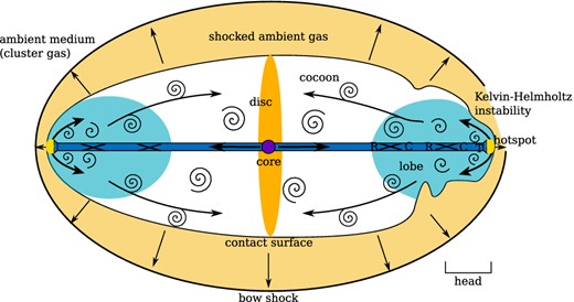
Schematic representation of the hydrodynamics of a disc galaxy with AGN jets. The beam (blue) emerges from the core containing the AGN. The jet plasma passes through regions of rarefraction (R) and compression (C) at internal shocks until it strongly decelerates at the terminal shock (T). The shocked plasma streams out of the hotspot high-pressure region (yellow) and forms a backflow. Vortices are generated and advected with the flow, inflating the cocoon (white inner region and light blue region). The outer parts of the cocoon, where radio-emitting electrons did not yet cool down, are visible as ‘lobes’. The overpressured cocoon drives a bow shock outwards into the ambient medium, forming a thick shell of shocked ambient gas. At this evolutionary stage, the bow shock has already overrun disc of the host galaxy. The picture is 90 deg rotated to the setup in the simulations.
Although the physical understanding of star formation is still limited and debated (Padoan & Nordlund 2011), it can be assumed that a pressurized disc can trigger gravitational instabilities, compress the galaxy's clouds, and push the densities within the disc above the critical density for star formation, thus resulting in an increased SFR. This picture is further supported by a few observations of well-resolved star-forming molecular clouds (Keto, Ho & Lo 2005; Rosolowsky & Blitz 2005) and by detailed simulation of the ISM (e.g. Slyz et al. 2005; Zubovas, Sabulis & Naujalis 2014).
While the simulations of Gaibler et al. (2012) resolved the jet interaction and the expansion of the blast wave more realistically, they were unable to examine the long-term effects of this pressurization and were lacking the necessary physics for these time-scales, most importantly gravity. Motivated by the observed pressurization of the disc from the outside found in their hydrodynamical simulations of AGN jet feedback, we have investigated the isolated effects of this extra pressure on a galaxy disc in an academic model, but on a much longer time-scale, by running hydrodynamical simulations with self-gravity, without AGN jets, but with simple prescriptions for external pressure such as that which may be caused by the jet cocoon. In a first study (Bieri et al. 2015), we simulated disc galaxies of one-tenth the total mass of the Milky Way, varying their initial gas fraction. We found that with a given level of external pressure, the disc fragments into numerous clumps, causing enhanced star formation. In this paper, we study the effects of external pressure in more detail, by considering different geometries and levels of external pressure, as well as studying the effects of supernova (SN) feedback and mass resolution.
In Section 2, we describe our suite of hydrodynamical simulations. Our results are presented in Section 3 and summarized in Section 4.
2 SIMULATION SET-UP
2.1 Basic simulation scheme
Our simulations begin with a galaxy made of a disc of gas and stars, a stellar bulge and a dark matter (DM) halo. We allow this galaxy to relax to an equilibrium configuration (with a reasonable disc thickness) over the rotation time of the disc at its half-mass radius. This first phase is performed without gas cooling, or star formation or feedback, in order to evacuate spurious waves emitted from the imperfect equilibrium of the initial conditions. After this first relaxation phase, we turn on the external pressure, gas cooling, star formation, and also feedback from supernovae (SNe), as described below.
The initial condition method introduced by Springel & Hernquist (2005) is used to generate the DM particles with an NFW (Navarro, Frenk & White 1997) density profile and a concentration parameter of c = 10. The virial velocity of the DM particles is set to be v200 = 70 km s− 1, which corresponds to a virial radius of R200 ≈ 96 kpc and a virial mass of |$M_{200} \approx 1.1 \times 10^{11}\, \rm \mathrm{M}_{\odot }$|. A Hubble constant of H0 = 73 km s− 1 Mpc− 1 is assumed. The star particles as well as the gas are distributed in a rotationally supported exponential disc with a scalelength of 3.44 kpc and scaleheight 0.2 kpc, and a spherical, non-rotating bulge with a Hernquist profile (Hernquist 1990) of scale radius 0.2 kpc. We use 106 DM particles with a mass resolution of 1.23 × 10⁵ M⊙ to sample the DM halo, and 5.625 × 10⁵ star particles sampling the disc of which 6.25 × 10⁴ star particles are used to sample the bulge. The stellar mass resolution is |$1.57 \times 10^{4}\, \rm \mathrm{M}_{\odot }$| for the 10 per cent gas fraction simulation (hereafter, gasLow) whereas for the 50 per cent gas fraction simulation (hereafter, gasHigh) the mass resolution is |$8.73 \times 10^{3}\, \rm \mathrm{M}_{\odot }$|. The relevant galaxy parameters are shown in Table 1.
Galaxy parameters: scale radius (rs), gas fraction (fg), total stellar mass (M*), and total gas mass in the disc (Mgas).
| Identifier | rs | fg | M* | Mgas |
|---|---|---|---|---|
| (kpc) | (per cent) | (109 M⊙) | (109 M⊙) | |
| gasLow | 3.4 | 10 | 8.1 | 0.9 |
| gasHigh | 3.4 | 50 | 4.6 | 4.4 |
| Identifier | rs | fg | M* | Mgas |
|---|---|---|---|---|
| (kpc) | (per cent) | (109 M⊙) | (109 M⊙) | |
| gasLow | 3.4 | 10 | 8.1 | 0.9 |
| gasHigh | 3.4 | 50 | 4.6 | 4.4 |
The gas density is truncated in the surface of a cylinder of radius rcut = 12 kpc (from the disc axis) and of height hcut = 2.5 kpc (above and below the disc). Beyond this cylinder, the density is set to be that of the circumgalactic medium (CGM), which is modelled with a constant hydrogen number density of nCGM = 10− 3 H cm− 3. The pressure and temperature profiles outside the disc are calculated assuming spherical hydrostatic equilibrium. For the relaxation phase, the simulations are run for one rotation period of the half-baryonic mass radius (5 kpc) of the galaxy, i.e. ≈ 0.5 Gyr.
The simulations are run with the ramses adaptive mesh refinement code (Teyssier 2002). Particles motions are evolved through the gravitational force with an adaptive particle mesh solver using a cloud-in-cell interpolation, together with the mass contribution of the gas component. The evolution of the gas is followed with a second-order unsplit Godunov scheme. We use the HLLC Riemann solver (Toro, Spruce & Speares 1994) with MinMod total variation diminishing scheme to reconstruct the interpolated variables from their cell-centred values. The box size is 655 kpc with a coarse level of 7, and a maximum refinement level of 14 corresponding to a Δx = 40 pc minimum cell size for most of the simulations. We used isolated boundary conditions for the Poisson solver and zero-gradient boundary conditions for the hydro solver. Given that the box size is ∼50 times larger than the galaxy radius, the galaxy is not affected by possible effects at the boundaries of the simulation box. For convergence studies, we perform a higher resolution run with a spatial resolution of Δx = 10 pc (maximum level of refinement 16). The refinement is triggered with a quasi-Lagrangian criterion: if the gas mass within a cell is larger than |$8 \times 10^{7}\, \rm \mathrm{M}_{\odot }$| or if more than 8 DM particles are within the cell a new refinement level is triggered.
2.2 Application of external pressure
After adiabatic relaxation (no gas cooling), the origin of time is reset to 0 and the base simulations are run further in time with the subgrid modelling of gas cooling, star formation and feedback, and with an enhanced and uniform pressure outside the disc (pressure simulations) for another ≈ 420 Myr. The pressure enhancement is applied at an instant starting at t = 0. This instant pressure increase is justified since the bow shock observed in the simulations of Gaibler et al. (2012) manages to pressurize the entire gaseous disc within a time-frame of only a few Myr. The pressure is enhanced by increasing the internal energy of gas cells according to two different criterions (i.e. two different configurations): either outside the sphere of radius r1 = 12 kpc (hereafter, p_spher), or else where the gas number density is lower than 0.014 H cm− 3 (i.e. right outside the disc component, hereafter, p_dens or equivalently gasHigh_d). The radius r1 is chosen to be the cutoff radius from the initial condition setup, whereas the densities for the p_dens simulations are chosen to be the radially averaged density at r1.
Primarily, the p_spher and p_dens models represent different numerical implementations and give an idea of the range of possible outcomes. However, the two different models also mimic the two different possible pressurizations of the disc due to the ram pressure (p_spher) from the backflow from the jet's high-pressure hotspot and the thermal pressure (p_dens) of the cocoon. This is illustrated in Fig. 1. In the p_spher simulation, the bow shock pressurizing the disc is assumed to be quasi-isotropic. The effect of isotropy of external pressure is compared with a simulation of a non-isotropic bipolar pressure increase in Appendix A.
For the case of external pressure in disc geometry (p_dens), we increase the pressure, only at time t = 0, at a value of pa Pmax wherever the gas density is below 0.014 H cm− 3. This gas density corresponds to a height of 1.1 kpc above and below the plane along the minor axis of the disc (R = 0).
In the simulations of Gaibler et al. (2012), the bow shock that pressurizes the disc reaches a maximum pressure of P ≃ 8 × 10− 11 Pa. This justifies our chosen pressure enhancement where the maximum pressure increase for the gasHigh (pa10) and gasLow (pa7) simulation corresponds to P ≃ 9.8 × 10− 12 Pa and P ≃ 3.2 × 10− 11 Pa, respectively.
The pressure profiles for one of the p_spher simulations (run pa3) before and after the pressure enhancement as well as its evolution over the simulation time are shown in Fig. 2. We can see that at 2.4 Myr, right after the restart of the simulation, the pressure smoothly rises from ∼ 10− 13 Pa at the centre up to 10− 11 Pa at a distance r = 13.5 kpc. At later times, this pressure enhancement propagates within the central region of the halo and connects to the galaxy.
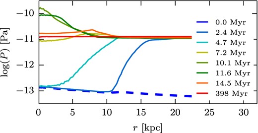
Mean pressure versus radius at different times (see legend) for the pa3 run of the gasHigh_fb set. The dashed line shows the pressure profile before the onset of external pressure. The pressures are averaged within spherical shells.
The relevant physical parameters for the pressure simulations are summarized in Table 2.
Physical parameters of runs: gas fraction (0.1 for gasLow and 0.5 for gasHigh), pressure amplification (pa), run with no-feedback (nf), run with feedback (fb), spatial resolution (Δx), and pressure geometry
| Identifier | Gas | pa | nf/fb | Δx | Geometry |
|---|---|---|---|---|---|
| fraction | (pc) | ||||
| pa01 ≡ nP | 0.1 | |$\checkmark$|/ |$\checkmark$| | 40 | ||
| pa04 | 0.4 | |$\checkmark$|/ |$\checkmark$| | 40 | ||
| pa08 | 0.8 | |$\checkmark$|/ |$\checkmark$| | 40 | ||
| pa1.2 | 1.2 | |$\checkmark$|/ |$\checkmark$| | 40 | ||
| pa1.5 | gasLow | 1.5 | |$\checkmark$|/ |$\checkmark$| | 40 | p_spher |
| pa3 | 3 | |$\checkmark$|/ |$\checkmark$| | 40 | ||
| pa5 | 5 | |$\checkmark$|/ |$\checkmark$| | 40 | ||
| pa7 | 7 | |$\checkmark$|/ |$\checkmark$| | 40 | ||
| pa01 ≡ nP | 0.1 | |$\checkmark$|/ |$\checkmark$| | 40 | ||
| pa01_hR ≡ nP_hR | 0.1 | x / |$\checkmark$| | 10 | ||
| pa02 | 0.2 | |$\checkmark$|/ |$\checkmark$| | 40 | ||
| pa04 | 0.4 | |$\checkmark$|/ |$\checkmark$| | 40 | ||
| pa08 | 0.8 | |$\checkmark$|/ |$\checkmark$| | 40 | ||
| pa1.2 | 1.2 | |$\checkmark$|/ |$\checkmark$| | 40 | ||
| pa1.5 | gasHigh | 1.5 | |$\checkmark$|/ |$\checkmark$| | 40 | p_spher |
| pa2 | 2 | |$\checkmark$|/ |$\checkmark$| | 40 | ||
| pa3 | 3 | |$\checkmark$|/ |$\checkmark$| | 40 | ||
| pa3_hR | 3 | x / |$\checkmark$| | 10 | ||
| pa5 | 5 | |$\checkmark$|/ |$\checkmark$| | 40 | ||
| pa7 | 7 | |$\checkmark$|/ |$\checkmark$| | 40 | ||
| pa8 | 7 | |$\checkmark$|/ |$\checkmark$| | 40 | ||
| pa10 | 10 | |$\checkmark$|/ |$\checkmark$| | 40 | ||
| pa01_d ≡ nP | 0.1 | |$\checkmark$|/ |$\checkmark$| | 40 | ||
| pa02_d | 0.2 | |$\checkmark$|/ |$\checkmark$| | 40 | ||
| pa03_d | 0.3 | |$\checkmark$|/ |$\checkmark$| | 40 | ||
| pa04_d | 0.4 | |$\checkmark$|/ |$\checkmark$| | 40 | ||
| pa08_d | 0.8 | |$\checkmark$|/ |$\checkmark$| | 40 | ||
| pa1.2_d | 1.2 | |$\checkmark$|/ |$\checkmark$| | 40 | ||
| pa1.5_d | gasHigh | 1.5 | |$\checkmark$|/ |$\checkmark$| | 40 | p_dens |
| pa2_d | 2 | |$\checkmark$|/ |$\checkmark$| | 40 | ||
| pa3_d | 3 | |$\checkmark$|/ |$\checkmark$| | 40 | ||
| pa5_d | 5 | |$\checkmark$|/ |$\checkmark$| | 40 | ||
| pa7_d | 7 | |$\checkmark$|/ |$\checkmark$| | 40 | ||
| pa10_d | 10 | |$\checkmark$|/ |$\checkmark$| | 40 |
3 RESULTS
In this section, we present our simulation results considering different isolated disc simulations with various pressure boosts outside the disc. We analyse our simulations regarding disc fragmentation, star formation, clump properties, and the galaxy's mass budget. We then compare our simulations with a simple theoretical implementation regarding the growth of the SFR and show that it scales approximately as a power just below unity of the external pressure. Finally, we calculate the KS relation and find that our toy model for AGN-induced overpressurization leads to the galaxies lying higher in the starburst region of the KS relation.
The effects of external pressure turn out to be similar whether or not SN feedback is included in the simulations. We will therefore only present, in this section, the results of the stellar feedback simulations. A comparison between the no-feedback and feedback simulations is provided in Appendix B.
3.1 Qualitative differences
Figs 3 and 4 show maps of the gas density for selected runs at different times, for the gasLow_fb and gasHigh_fb as well as gasHigh_d_fb runs, respectively, and for two cases without external pressure boost nP and with extra pressure pa3. Comparing the nP runs, we observe that the gas is clumpier in the gasHigh_fb simulation than in the gasLow_fb run. We will show in Section 3.2 that this is a simple consequence of the Toomre instability. The increased pressure leads to accelerated clump formation for the gasLow_fb, gasHigh_fb, gasHigh_d_fb simulations, and a clumpier ISM in all cases. Generally less gas between clumps in the enhanced pressure runs, in all the gasLow_fb, gasHigh_fb, and gasHigh_d_fb cases can be seen.
Gas density maps (mass-weighted) of two of the gasLow_fb simulations without enhancement of the external pressure nP (top row), and with enhancement of the external pressure pa3 (bottom row). The different columns show different times as labelled. Each panel shows both face-on (40 × 40 kpc, upper part) and edge-on (40 × 20 kpc, lower part) views. One can see that an increased pressure outside the galaxy leads to accelerated clump formation and less gas between the clumps.

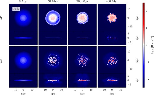
Gas density map (mass-weighted) for a selection of the gasHigh_fb and gasHigh_d_fb simulations, for no pressure enhancement (top), and for a pressure enhancement of pa3 (middle for gasHigh_fb and bottom for gasHigh_d_fb). The density scale is as in Fig. 3. An increased pressure outside the galaxy leads to accelerated clump formation and less gas between the clumps. The morphological structure of the two simulations with two different ways to increase the pressure (gasHigh_fb, and gasHigh_d_fb) is slightly different, but only in the outskirts of the galaxy. The edge-on view shows a mass outflow for all the simulations.
In Fig. 4, one can compare the two different ways to increase the pressure (p_spher, p_dens). The morphological structure of the two simulations gasHigh_fb and gasHigh_d_fb is slightly different. Fewer clumps are seen in the gasHigh_fb run than in the gasHigh_d_fb run. It seems, however, that the clumps are only missing in the outskirts of the gasHigh_fb galaxy, whereas a similar amount of clumps can be detected in the centre. The edge-on views indicate that in the gasHigh_fb simulations, a large amount of mass flows out of the galaxy due to the pressure increase, while in the gasHigh_d_fb simulations the mass outflow seems to be less extended. We will quantify the mass outflows in the different runs in Section 3.5.
3.2 Disc fragmentation
Since the star formation recipe depends on the local gas density (see equation 1), we expect enhanced star formation when more clumps are formed (as the gas gets more concentrated), assuming that the clumps have sufficient mass. Therefore, if an increased pressure leads to increased fragmentation and hence increased clump formation, we expect star formation to be positively enhanced when external pressure is applied to the galaxy. We first consider the fragmentation by counting the high-density clumps. We detect the clumps in the simulation by running the clump finder described by Bleuler & Teyssier (2014). This method identifies all peaks and their highest saddle points above a given threshold (21 H cm− 3). A clump is recognized as an individual entity when the peak-to-saddle ratio is greater than 1.5; otherwise the density peak is merged with the neighbour peak with which it shares the highest saddle point.
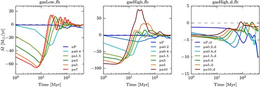
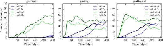
The visual impression of increased clump formation when external pressure is applied on the galaxy (Figs 3 and 4), is confirmed when looking at the number of clumps as a function of time. Fig. 5 shows the number of clumps as a function of time for the gasLow_fb (left-hand panel), gasHigh_fb (middle panel), and gasHigh_d_fb (right-hand panel) simulations, respectively.
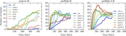
Time evolution of the number of clumps for a selection of simulations with SN feedback: gasLow_fb (left), gasHigh_fb (middle), and gasHigh_d_fb (right) simulations. The lines are smoothed with a Blackman–Harris window with a width of |$2 \sqrt{{\rm len(array)}}$|, where len(array) is the number of points. The clumps were extracted with the Bleuler & Teyssier (2014) algorithm, with a density threshold of 21 H cm−3 and a peak-to-saddle threshold of 1.5. The maps show that an increased pressure leads to increased clump formation and the increase in clump number is dependent on the pressure applied on to the galaxy. Beyond a certain pressure enhancement, the number of clumps decreases or remains very similar for higher pressure runs.
In the gasLow_fb run, the number of clumps is constantly increasing with time, regardless of the amount of external pressure. Clump formation starts earlier in the runs with external pressure. However, the number of clumps at a given time is not a monotonic function of external pressure: at low external pressure (up to pa3), the number of clumps at given time increases with increasing pressure, while the reverse trend occurs for external pressures above 3 Pmax.
The general effect that more clumps are formed in the simulations with external pressure is similar for the gasHigh_fb and gasHigh_d_fb runs. Similar to the gasLow_fb simulation, the number of clumps increases with increasing pressure up to a certain pressure (pa5) and then decreases again for the gasHigh_fb simulation and stays at the same level for the gasHigh_d_fb simulation. For the lower pressure as well as the non-pressure simulations, the number of clumps increases with time. However, for higher pressure simulations, the number of clumps reaches a plateau at late times. For the gasHigh_fb runs, the initial rise in the number of clumps is fastest for the pa3, pa5 and pa7 cases, but in the pa3 case the number of clumps reaches its plateau at a later time, hence at a higher level.
The time evolution of the number of clumps for the gasHigh_d_fb simulation is roughly similar to the gasHigh_fb simulation. At early times, the rise in number of clumps is fastest for the high-pressure runs. The number of clumps keep rising with time for the lower pressure enhancements, while it reaches a maximum for the higher pressure enhancements. The time when the number of clumps reaches its plateau is also shortest for higher external pressures. After 300 Myr, there is no clear trend in number of clumps versus external pressure for the higher pressure runs. The increase of clump number is therefore highly dependent on the pressure applied on the galaxy. However, beyond a certain pressure enhancement (pa5_d), the number of clumps remains very similar for higher pressure runs. After ≈ 300 Myr the number of clumps is roughly independent of external pressure for the gasHigh_fb and gasHigh_d_fb simulations.
In the gasLow_fb run with no external pressure, only a single clump in the entire disc is formed, at late times (350 Myr), when the gas has sufficiently collapsed to reach the clump gas density threshold. On the contrary, in the gasHigh_fb run, the number of clumps increases up to ≃ 35, even without any forcing by the external pressure.
The difference between the gas-poor and gas-rich galaxies, before the external pressure is applied, is that the gaseous disc is Toomre-stable against small-scale fragmentation in the gas-poor case: the mean Toomre parameter 〈Q〉 = 〈cs κ/(πG Σgas)〉 = 3.29 > 1; on the other hand, the gas-rich disc is Toomre-unstable (〈Q〉 = 0.72 < 1). Here, Σgas is the surface density, cs is the sound speed, and κ is the epicyclic frequency (measuring the shear of the rotating disc). Therefore the gasLow_fb simulations demonstrate that fragmentation of the galactic disc can be driven by the forcing of an external pressure, even though the disc is initially Toomre-stable.
3.3 Star formation history
In Section 3.2, we have seen that an increased pressure enhancement leads to an increased number of clumps up to a certain value of pressure and then a typically lower number of clumps thereafter. Since the gas density threshold of clump detection is set to be above that for star formation, one expects that the star formation history should evolve in a similar fashion to the evolution of the number of clumps.
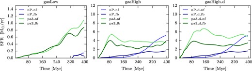
Fig. 6 shows that the star formation histories of the different runs indeed resemble the time evolution of the number of clumps previously shown in Fig. 5. In particular, at early times in the runs with gasHigh higher pressures lead to higher SFRs. But with high pressures, the SFR saturates earlier. In the gasHigh_fb runs, the maximum SFRs in the high-pressure runs are lower than in the other runs, while in the gasHigh_d_fb runs, the maximum level of SFR is reached for the three highest pressures, while the SFRs at later times (300 Myr) are roughly independent of the external pressure.
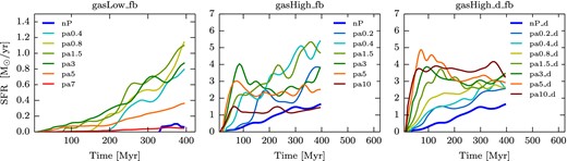
SFR for a selection of the simulations with SN feedback: gasLow_fb (left), gasHigh_fb (middle), and gasHigh_d_fb (right) simulations. The lines are smoothed as in Fig. 5. This figure shows that higher pressures lead to higher SFRs. For the higher pressure enhancement simulations, the SFR reaches a maximum or plateau at later times for the gasHigh_fb, and gasHigh_d_fb simulations. After a certain pressure increase, the SFR decreases or stays at the same level for all the simulations and hence the runs with intermediate pressure generally produce the highest SFR at all times.
In the gasLow_fb runs, while the nP case leads to star formation only after a long time delay (330 Myr), the highest pressures, although leading to immediate but small levels of star formation, are unable to generate substantial star formation from the earliest times. The runs with intermediate pressures produce the highest SFR at all times. We will show in the next sections that this is due to the low mass-outflow of the intermediate pressure simulations that allows the clumps to increase in density. Conversely, larger external pressures lead to such strong pressure waves that the gas is removed from the galaxy. This prevents the formation of large clumps and tends to suppress the star formation.
The effect of the external pressure on the SFR is even more significant when looking at the gasHigh_fb simulations (middle panel of Fig. 6). The SFR of the no-pressure simulation slowly increases after a certain time, whereas the SFR increases faster when pressure is applied: it reaches a maximum at a certain rate and more or less maintains this rate for the remaining of the simulation. Towards the end of the simulation, the SFR of the no-pressure simulation catches up, again similarly to the clump number behaviour. The SFR for the gasHigh_d_fb simulation (right-hand panel of Fig. 6) behaves quantitatively similar to the gasHigh_fb simulation. One can see that the SFR in these simulations reaches the maximum or plateau at later times than in the corresponding gasHigh_fb simulations. The rapid rise of the SFR reaches increasingly higher levels of peak SFR with higher external pressure up to pa5_d, while pa10_d reaches a slightly lower maximum SFR.
The left-hand panels of Fig. 6 show that the SFRs of the gasLow simulations start with a significant time delay, and the maximum enhancement of the SFR relative to the nP run is highest (∼12) at the end of the simulation (after 400 Myr). On the other hand, the corresponding SFR enhancements for the higher gas fraction simulations (middle and right-hand panels of Fig. 6) are lower (∼ 3.5 for gasHigh and ∼1.5 for gasHigh_d) at the end of the simulation (after 400 Myr) than at the beginning (∼40 for gasHigh and ∼70 for gasHigh_d at ∼80 Myr) of the simulation. External pressure thus first produces a significantly higher SFR in comparison to the simulation with no external pressure. But the duration of this large SFR enhancement for the gasHigh and gasHigh_d simulations is shorter than that of the gasLow simulation. The free fall time of the higher density gas is shorter than the free fall time of the low-density gas which leads to the gas collapsing early on, whereas a delay is expected for the lower gas fraction disc.
3.4 Clump properties
Star formation requires a significant supply of cold gas as well as the fragmentation of the disc into clumps that carry a sufficient amount of gas to form stars. On the other hand, one can argue with the Jeans and Toomre instability arguments if indeed an increased pressure outside the galaxy that later increases the pressure inside the galaxy leads to higher densities, as well as a possible expulsion of disc gas depending on the momentum carried by the pressure wave coming into the disc. The competition between higher densities and mass outflow will influence the amount of gas within the clumps.
For the gas-rich disc simulations, we saw (Fig. 5) that, at the very beginning, when the pressure wave comes into the galaxy, the number of clumps is highest for the highest pressure. While the clumps are more numerous with the highest pressures, it is worthwhile knowing whether their masses are affected by the external pressure.
Fig. 7 shows the modulation of the average clump mass rises with external pressure at three times of the simulations. At early times (top panel), the clump masses for the gasHigh simulations (gasHigh, centre panel, and gasHigh_d, right-hand panel) are higher the greater the external pressure. At later times (middle and bottom panel), the clump masses are roughly independent of the external pressure applied, probably because the disc gas has been either already accreted on to the clumps or expelled out of the galaxy (see discussion below), leaving no more diffuse gas available for accretion on to the clumps. The time at which the diffuse gas is either consumed on to the clumps or expelled must happen earlier for the higher external pressure simulations as the fragmentation happened earlier for these simulations. This explains the different times when the SFR reaches a plateau, occurring earlier the higher the pressure. In the gasHigh_fb runs at high external pressures, fragmentation is not the only cause of SFR (since there is a maximum pressure enhancement beyond which the SFR is lower), meaning that the gas supply is more critical, and not always available despite the high gas fraction. This suggests that the mass flow out of the galaxy also plays an important role. And indeed, the mass outflow is very efficient for pa7 and pa10 after 30 Myr. We will discuss this in detail in Section 3.5, below.
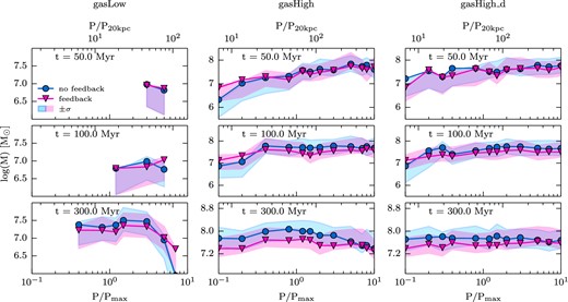
Average clump mass for the gasLow_fb (left), gasHigh_fb (middle), and gasHigh_d_fb (right) simulations. The blue line with round markers correspond to the no-feedback simulations, whereas the pink line with triangles corresponds to the feedback simulations. The shaded green/blue area shows the area of mass containing ±σ of the density PDF for the no-feedback/feedback simulations. In the bottom and top of each subfigure, the x-axis shows the P/Pmax and P/P20 kpc values, respectively, where Pmax is the maximum pressure inside the disc and P20 kpc is the averaged pressure at 20 kpc. At the beginning of the simulation, the clump masses for the gasHigh simulations are higher the greater the pressure for the gasHigh simulations. At later times, the clump masses are roughly independent of the external pressure. For the gasLow simulation, the clump mass does not increase with higher external pressure but rather decreases or stays at approximately the same level.
In the p_dens simulations, there is a maximum pressure enhancement (pa5_d) beyond which the SFR remains at approximately the same level without decreasing. As we will see in Section 3.5, mass outflows are also absent. The high gas fraction leads therefore to higher density enhancement by external pressure, hence both number of clumps and SFR are highest when the external pressure is high. However, there only is a limited amount of gas available in the galaxy. One can assume that the limited gas supply is insufficient for more star formation, so the SFR remains at the same level independently of the pressure enhancement.
Fig. 7 shows that, for the gasLow simulations (gasLow, left-hand panel), the clump mass does not increase with greater external pressure, but rather decreases at early times (top panel). At later times, the clump mass is roughly independent of the pressure up to pa3, beyond which the clump mass decreases. This is the same pressure enhancement which leads to the highest SFR. As we will see in Section 3.5, the gasLow galaxies suffer from strong gas outflows that reduce the supply of gas available for clump buildup, leading in turn to smaller clump masses within the galaxy.
In Fig. 7, the difference in clump masses for the feedback and no-feedback simulations can also be seen for all the simulations. At early times, there is no significant difference between the no-feedback and feedback simulations. At later times, the difference in clump masses becomes more apparent for both the high gas fraction and gasLow simulations. One can see that the clump masses for the feedback simulations are lower at the end of the simulation than for the no-feedback simulations, independent of the pressure increase. Because the feedback increases the porosity of the ISM that in turn counteracts the formation of clumps (Silk 2001), the observed smaller clump masses for the feedback simulations are expected. This difference is more dominant in the gasHigh simulation as can be seen in the left-hand panel of Fig. 7. The similar mean clump masses in the feedback and no-feedback runs at the beginning of the simulation appears to be a consequence of the implementation of the SNe in the simulation. As discussed above, an SN explosion occurs 10 Myr after the birth of the star particle. The first stars form shortly before 50 Myr and one would therefore not expect to see a large difference between the feedback and no-feedback simulations. At 100 Myr, some stars exploded into SNe, but only constitute a small fraction of all stars, hence the small difference between the feedback and no-feedback simulations at this stage.
It is interesting to look at the probability density function (PDF) at different times of the simulations in order to better understand the observed SFR behaviour. The PDF can be seen in Fig. 8 for two different times for a selection of the gasLow (left), gasHigh (middle), and gasHigh_d (right) simulations. Increasing external pressure allows one to reach higher gas densities faster, which is in agreement with the SFR behaviour we have seen previously. For the gasHigh simulations, the nP simulation slowly catches up with the overpressure simulations similar to the SFR behaviour. For the gasLow simulation, the no-pressure simulations never attain the densities reached by the moderate pressure enhancement simulations. The high-pressure simulation (pa7) also never reaches high gas densities, which is due to the removal of gas within the galaxy, as we will discuss in Section 3.5, below. It can be seen in Fig. 8 that over the course of the simulation a high-density power law with a slope between −7/4 (or even steeper) and −3/2 develops, especially for the high gas fraction simulations. A comparable power-law range has been found in observations (e.g. Kainulainen et al. 2009, Lombardi, Lada & Alves 2010) and simulations including gravity and turbulence (e.g. Kritsuk et al. 2011) where they argue that the origin of the power-law tail is due to self-similar collapse solutions.
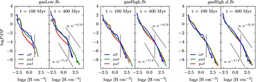
Density PDF at different times for a selection of the gasLow_fb (left), gasHigh_fb (middle) and gasHigh_d_fb (right) simulations. The threshold (14 H cm− 3) for star formation is plotted as a grey vertical line. One can see that greater external pressure allows the galaxy to reach higher densities on a faster time-scale. The nP simulation slowly catches up with the overpressure simulations for the gasHigh, whereas this is not the case for the gasLow simulation. For the gasLow simulation, the high-pressure simulation (pa7) never reaches the high densities. As indicated with the grey power-law lines one can see that over the course of the simulation a slope between −3/2 and −7/4 (or even steeper) develops at high densities. This is in agreement with simulations including gravity and turbulence done for instance by Kritsuk, Norman & Wagner (2011).
3.5 The galaxy's mass budget
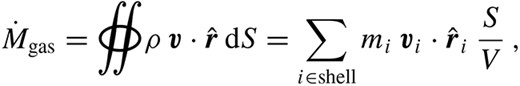
The mass flow rate (MFR) as well as the total amount of newly formed stars plus dense gas should provide us a better understanding of the star formation history described above. In particular, one would like to understand why there seems to be an optimal external pressure enhancement for star formation, beyond which the SFR ends up at lower values.
Time evolution of the MFR for selected runs from the gasLow_fb (left), gasHigh_fb (middle) and gasHigh_d_fb (right) simulations. Negative (positive) values of the mass outflow rate denote a net mass inflow (outflow). One can see a difference in the MFR between the different ways pressure is put on the galaxy (gasHigh_fb, gasHigh_d_fb). Due to the pressure gradient in the p_spher simulations, the pressure wave coming into the galaxy carries a lot of momentum that leads to a mass inflow followed by a mass outflow for the higher pressure simulations. This mass outflow is negligible for the p_dens simulations due to the pressure wave carrying very little momentum. For the most extreme case, the expelled mass reaches 80 per cent of the initial gas mass for the highest external pressure simulation of gasHigh_fb.
In all three sets of simulations, external pressure leads to mass inflow at early times. This early mass inflow is large but different for the different ways pressure is applied on to the galaxy. In the p_spher simulations, the pressure is applied outside the galaxy in a low-density medium leading the pressure to have a larger negative pressure gradient than in the p_dens simulations where the pressure is applied close to the galaxy and therefore in a higher density environment. The pressure gradient leads to a force acting inwards that leads to the force sweeping the gas inside the yet unaffected low-density regions of the CGM. This allows the pressure wave of the p_spher simulations to carry more mass and momentum from the ambient hot medium in comparison to the pressure wave of the p_dens simulations.
This explains the larger mass inflow observed in the p_spher simulations (left and middle panels of Fig. 9) compared to that at the start of the p_dens simulation. With its larger momentum, the mass inflow of the p_spher pressure wave is followed by a short period of mass outflow (for both low and high gas fractions). This reflecting wave is the analogy of a 1D experiment of a shocked wind (the inflowing gas swept by the extra-pressure wave) on to a reflective boundary (the high-density gas of the galaxy). This mass outflow is negligible for the gasHigh_d_fb simulations, since the pressure wave carries very little momentum.
For the p_spher simulation sets, higher external pressures lead to stronger maximum inflows at early times and to stronger maximum outflows at later times. In addition, in the simulations with high external pressures (pa7 and pa10), the mass outflow that follows the mass inflow occurs very rapidly (in less than 20 Myr). After these two phases of important mass inflow/outflow, the MFR oscillates around zero for both the gasLow_fb and gasHigh_fb simulations with pa < 5. In contrast, in the gasHigh_d_fb simulations, the MFR depends little on the external pressure.
We stress, however, that the pressure and no-pressure p_dens simulations do not differ significantly and that, overall, there is little net mass flow. This most likely explains why the SFR of the p_dens simulations is smoother and less noisy when compared to the p_spher simulations of the same gas fraction (gasHigh).
In order to understand the galaxy's mass budget better, we look at the time evolution of the total mass of newly formed stars plus dense (n > 0.1 H cm− 3) gas. Mtot = Mtot,starsN + Mtot,gasD is shown relative to the initial galaxy gas mass (total not just dense), Mtot,gas0 (see Table 1) shown in the top panel of Fig. 10. Mtot,starsN and Mtot,gasD are shown in the middle and bottom panels, respectively. The initial value of Mtot/Mtot,gas0 is below unity at t = 0 since the gas density in the galaxy is not everywhere above n > 0.1 H cm− 3, especially in the outskirts of the disc and for the gasLow galaxy. In the absence of extra external pressure (nP runs), the ratio Mtot/Mtot,gas0 quickly moves significantly beyond unity as the gas cooling allows to reach the gas densities above n > 0.1 H cm− 3. The gas cooling also takes place in the CGM that feeds the galaxy with some extra gas. The extra mass of gas from the mass inflow and from the gas cooling adds more significantly to the low gas fraction galaxy because of its lower initial gas mass, which explains why the increase in SFR is more significant in the gasLow runs than in the gasHigh runs. Comparing the top panel with the middle and bottom panels, one sees that dominates the total mass budget of the disc for the low gas fraction simulations. For the higher gas fraction simulations, the mass of stars plays a role for the low external pressure simulations. For the p_dens simulations the fraction of stars affects the SFR at late times in the simulation.
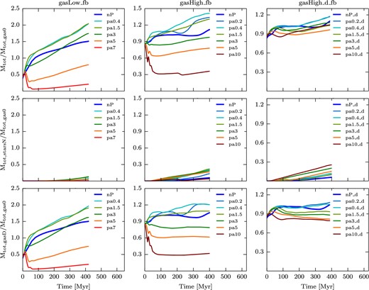
Time evolution of the mass in newly formed stars plus dense gas (n > 0.1 H cm− 3) (top), newly formed stars (middle), and dense gas (bottom) relative to the initial gas mass for a selection of the simulations with SN feedback: gasLow_fb (left), gasHigh_fb (middle), and gasHigh_d_fb (right) simulations. The lines are smoothed as in Fig. 5. Due to the mass inflow shown in Fig. 9, at the beginning of the simulation more mass can end up in the galaxy. This extra mass of gas is more significant for the gasLow galaxy for both the no-pressure and low-pressure enhancement simulations. For high-pressure enhancement in the gasLow simulation, the incoming pressure wave significantly disperses the galactic gas. The evolution of Mtot is similar for the gasHigh_fb simulation albeit with less mass variation. For the gasHigh_d_fb simulations, no significant mass variation within the galaxy due to pressurization is observed. Comparing the top, middle and bottom panels, one sees that for the low gas fraction simulations, gas dominates the total mass budget of the galaxy. For the higher gas fraction simulations, the mass of the stars plays a role for the low-pressure enhancement simulations.
For the gasLow simulations, intermediate regimes of forced external pressure (from pa0.4 to pa3) also show values of Mtot/Mtot,gas0 above 1 with values comparable to the nP run. Therefore, the increase in SFR (an order of magnitude above nP) is to be attributed to the extra compression of the ISM and exploration of larger gas densities with shorter collapsing time-scales (see Fig. 8). In contrast, higher pressurization values of the ISM (pa5 and pa7) lead to strong gas removal due to the incoming pressure wave that manages to significantly disperse the galactic gas. Since the gas reservoir is reduced, the SFR is also suppressed compared to more intermediate regimes of pressurization, but the overall SFR is still larger than in the nP case, where gas fragmentation is not reached.
The evolution of Mtot/Mtot,gas0 in the p_sphergasHigh galaxy behaves similarly to that for the gasLow galaxy, although with lower mass variation. It starts below unity for all pressures, and decreases even more for the high pressure increases (pa5 and pa10), because of the large mass outflows observed for those runs. This shows that the large mass outflows associated with high pressures prevent star formation. On the other hand, Mtot/Mtot,gas0 keeps rising for the lower pressure enhancements, showing that because no large mass outflow is observed, more stars can be formed. The Mtot/Mtot,gas0 curve is higher when a small pressure is applied outside the galaxy compared with the no-pressure simulation. In the case of p_dens overpressurization, there is no significant (<20 per cent relative) mass variation in the galaxy. Thus, the early fragmentation due to the increased pressure drives the different SFR levels for the different pressure simulations.
3.6 The SFR
Fig. 11 illustrates how the SFRs of different pressure simulations compare with one another at different times. For the gasLow, gasHigh, and gasHigh_d simulation sets, the SFR increases with increasing external pressure until a maximum is reached and then decreases again or stays at a similar level as for the gasHigh_d simulations. Also, no significant difference in the SFR can be seen between the feedback and no-feedback simulations, indicating that the external pressure increase is the dominant effect driving the increased SFR.
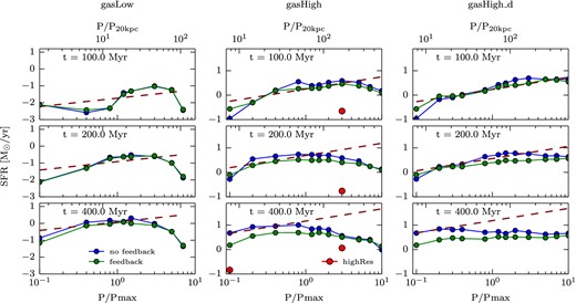
Time evolution of the SFR for all the gasLow_fb (left), gasHigh_fb (middle), and gasHigh_d_fb (right) simulations. Here, the no-feedback simulations are shown in blue and the feedback simulations are shown in green. The red points are the corresponding points from the highRes runs. The calculation of the SFR at a given time has been performed on the smoothed data. The SFR data are smoothed as in Fig. 5. The dark red dashed straight lines correspond to visual fits with a slope 9/10th to guide the eye. One can see that for higher gas fraction simulations, the SFR increases with external pressure and follows a power 9/10th of the external pressure. At later times, this is only true up until a certain external pressure. For the low gas fraction simulation, the SFR growth rate does not scale with power 9/10th of the external pressure.
In order to compare with the prediction explained below, a dark red dashed curve is plotted to guide the eye in Fig. 11 representing a power 9/10th fit of the SFR as a function of the external pressure applied on the galaxy. One sees that, for the gas-rich gasHigh and gasHigh_d simulations, the SFR follows a power 9/10th of the external pressure very well. At later times, the 9/10th power law is only fulfilled until the optimal pressure is reached. For the gasLow simulations, the SFR does not scale well with the 9/10th power of the external pressure. But as explained below, this was not unexpected.
The bright red points in Fig. 11 are the corresponding points from the highRes run. As can be seen in Appendix C, the formation of stars in the highRes run shows a delay compared to the lowRes run. This is due to the increase in star formation threshold for the higher resolution run. Because of this delay, one can also see a delayed behaviour of the SFR of the highRes run in Fig. 11. However, at later times, the highRes simulation shows a similar behaviour to the lowRes simulation.
The clumps, which have started forming at t = 0 because the disc is initially Toomre unstable (Fig. 12), are compressed when they are hit by the pressure wave. Since the disc gas does not cool significantly when the pressure wave hits the disc (the ratio of clump size to external sound speed is shorter than the clump cooling time), it is reasonable to assume adiabatic clump evolution. One then expects that density will rise as the power 1/γ of the pressure, hence, according to equation (5), |$\dot{\rho }_\ast \propto P_{\rm ext}^{3/(2\gamma )}$|. Therefore, for γ = 5/3, one finds |$\dot{\rho }_\ast \propto P_{\rm ext}^{9/10}$| for a given clump.
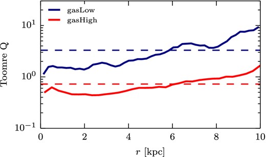
Local Toomre parameter for the relaxed disc at t = 0 for the gasLow and gasHigh simulations. The dashed line shows the mean Toomre parameter of the disc for the gasLow simulation 〈Q〉 = 3.29 > 1 and for the gasHigh simulation 〈Q〉 = 0.72 < 1. One therefore expects the gasHigh simulation to fragment independently of external pressure enhancement, whereas the gasLow simulations are not expected to fragment into many clumps. The fact that the pressur-enhanced simulations of the gasLow galaxies shows a significant increase in the number of clumps compared to no-pressure enhancement demonstrates that external pressure can stimulate the fragmentation of a disc even if it is Toomre-stable.
Finally, since most of the star formation happens within the dense regions it is safe to assume that most of the star formation happens within the clumps. We hence expect the total SFR of the disc to vary as |$P_{\rm ext}^{9/10}$| which matches the modulation of the SFR measured in our simulations with external pressure. After around 100/200 Myr, the assumption of adiabatic evolution is no longer valid, especially for the high-density clumps for which the temperature cools down faster and reaches the temperature floor Tfloor.
Admittedly, this approximation is crude because the clumps are still forming when the pressure wave hits the gasHigh and gasHigh_d discs. Also, our adiabatic approximation neglects the possible role of turbulence, for example induced by SN explosions (Silk 2001; Silk & Norman 2009; Silk 2013), in modulating the SFR in clumps. But we notice that, in our simulations, the relation between the disc SFR and the external pressure is only weakly affected by the presence of SNe (compare the no-feedback and feedback points in Fig. 11), which explains why the adiabatic evolution of clump densities appears to explain the modulation of disc SFR with external pressure of Fig. 11.
Hence, we expect that AGN-induced pressure should provide a boost of the SFR, independently of any possible increase in star formation efficiency, and initially roughly vary as the power 0.9 of the external pressure.
3.7 The KS relation
The KS law (Kennicutt 1998) relates the SFR per unit area as a power of the surface density of gas. This relation holds over several orders of magnitude in both quantities (Krumholz, Dekel & McKee 2012, and references therein), with the same normalization for global galaxies (including high-redshift ones; Genzel et al. 2010) and giant molecular clouds in the Milky Way (Heiderman et al. 2010; Lada, Lombardi & Alves 2010) and in the nearby M51 galaxy (Kennicutt et al. 2007). This demonstrates the remarkable universality of the SFR. At high redshift, starburst galaxies lie above the KS law for normal galaxies (Genzel et al. 2010). While the cause of this observed offset is not known, one may speculate that this increased SFR may be caused by positive AGN feedback.
Fig. 13 shows the KS relation at different times for several simulations for the three cases of gasLow_fb, gasHigh_fb, and gasHigh_d_fb with the observed relation from Daddi et al. (2010) overplotted. One can see that, over the course of 400 Myr, all runs lead to an increase in ΣSFR, by one to two dex, with much smaller variations (less than 0.3 dex) in Σgas. In particular, the runs with high gas fraction (with or without external pressure) show a decrease in Σgas. This decrease in gas surface density is related to the gas mass outflow at late times (Fig. 9) and to the consumption of gas by star formation. For the gasLow simulation, the evolution of Σgas is tied to the evolution of the total baryonic mass within the galaxy shown in Fig. 10. The light blue and green lines in Fig. 13 show the highRes simulations for the nP and pa3 set, respectively. One can see that the trends of the highRes simulation are very similar to the trends of the lowRes simulations, specifically at late times. Especially for the pa3 highRes simulation, one can see that higher gas densities are reached due to the higher resolution which allows the gas to collapse even further.
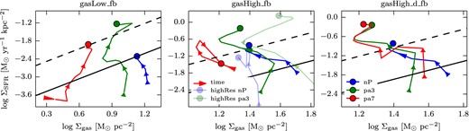
KS relation for selected runs (nP, pa3, pa7 with blue, green and red curves, respectively, with lighter colours for the runs with four times higher spatial resolution) from the gasLow_fb (left), gasHigh_fb (middle) and gasHigh_d_fb (right) simulations at 16 different times in colour. The evolution in time is shown with arrows. The 16 different times are equally spaced between tstart = 25 Myr and tend = 400 Myr. The circle shown corresponds to tend of the simulation with the corresponding colour. Data from Daddi et al. (2010) for the starburst (dashed line) and quiescent (solid line) sequences are overplotted for reference. For all the simulations, independently of the gas fraction, the simulations with external pressure lie closer to the starburst sequence than the no-pressure simulations. This shows that our toy model for AGN-induced star formation might be a possible explanation for explaining the increased number of starburst galaxies observed in the distant Universe.
For all the simulations independently of the gas fraction, the simulations with external pressure end up being pushed closer to or further beyond the starburst sequence than the corresponding simulations without external pressure. This trend is not changed for the highRes runs. Runs with external pressures leading to higher SFR also have a higher ΣSFR and therefore end up even closer to the starburst sequence. For instance, for the p_spher simulations, the pa7 run does not extend as far beyond the observed starburst sequence as the pa3 run, which reaches higher SFR for both the gasLow_fb and gasHigh_fb simulations (Figs 6 and 11). This is not as significant for the gasHigh_d_fb simulations as they do not experience a decrease of SFR but rather that the SFR stays at a certain level after a certain pressure increase (∼ pa5). We therefore see for this simulation set that the KS relations end in a very similar parameter space.
We conclude that this toy model for AGN-induced overpressurization plausibly leads to AGN-associated star-forming galaxies having enhanced specific SFRs, for example as suggested by recent observations, cf. (Zinn et al. 2013; Drouart et al. 2014).
4 CONCLUSIONS
It is a fascinating challenge to understand the extreme SFRs observed for some high-redshift galaxies, typically with luminous AGN and massive outflows: are these caused by higher contents of molecular gas or by a greater efficiency of star formation relative to this molecular gas content? Is turbulence sufficient to explain the high SFR values, or do we need recourse to a more exotic pathway that enhances SFRs even more? The latter option is motivated by the increasing evidence for the role of AGN in star formation, and in particular their role in a putative phase of positive feedback that accompanies or even precedes the commonly observed massive, star formation-quenching, outflows stimulated by AGN activity.
Using hydrodynamical simulations of isolated disc galaxies embedded in a hot overpressurized halo, we have been able to study the response of the galaxy SFR to the forcing exerted by this external gas pressure on to the disc. The pressure enhancement triggers instabilities leading to more fragmentation when compared to the no-pressure simulations (Figs 3 and 4). The enhanced fragmentation leads to the formation of more clumps (Fig. 5) as well as larger values of SFR (Fig. 6). This hints at a positive effect of the pressurization of the disc and therefore to positive feedback.
We observe a difference in the behaviour for the different ways in which the pressure is applied. In the simulations where external pressure is continuously applied beyond a certain radius (p_spher simulations), we observe an optimal pressure beyond which the number of clumps as well as the SFR is decreased. For the simulations where the pressure is instantaneously applied using a density threshold (overpressure applied closer to the galaxy disc), such an optimal pressure is not observed.
We have seen that the mass outflow plays a role in explaining this optimal pressure. In particular, for the gasHigh_fb simulations, a significant amount of gas gets expelled out of the galaxy, leaving little gas left to form stars and thereby lowering the SFR. The difference in SFR between the high and low external pressures for the gasLow_fb simulations is explained by the stagnation of the accumulation of mass in the clumps, which is again related to the large amount of gas that is removed by the incoming pressure wave. Our simulations have been tested with respect to the resolution and local presence or absence of SN explosions: the overpressurization of the disc still leads to a positive feedback effect (enhanced SFR).
We found that at given times of the p_spher simulations, the SFR (and its mean growth rate) vary as the power 9/10th of the applied pressure. We explain this by adapting the Schmidt law for the SFR as a function of 3D gas density for the inclusion of extra pressure caused by the AGN bow shock-driven radio lobe or wind, leading to compression times typically an order of magnitude shorter than the dynamical time, as argued by Silk & Norman (2009).
Though our setup of the extra pressure exerted by circumgalactic gas on to the galaxy is crudely modelled to mimic the pressure confinement by AGN activity, we are confident that such a mechanism could operate in more realistic configurations (see the jet simulations of Gaibler et al. 2012). We have demonstrated that such pressure confinement of the ISM drives the galaxy into an intense star formation regime, and could explain observations of star formation-enhanced galaxies in the presence of jet activity (Zinn et al. 2013). Cosmological simulations of pure AGN jet feedback in galaxy clusters (Dubois et al. 2010) have shown that it has a negative impact on the galaxy SFR on the long term, though these simulations were lacking spatial resolution in order to properly capture the small-scale fragmentation of the ISM. Our more global picture could suggest a two-stage mechanism for AGN feedback: a compression phase leading to a short burst of star formation, together with the expulsion or heating of the circumgalactic gas leading to a suppression of the gas accretion on to the galaxy and its star formation on longer time-scales. This remains to be verified with simulations of galaxies embedded in a cosmological environment with high spatial resolution and a self-consistent treatment of AGN feedback. We defer this study to future work.
YD and JS acknowledge support hosted by UPMC – Sorbonne Universités and JS for support at JHU by National Science Foundation grant OIA-1124403 and by the Templeton Foundation. RB has been supported in part by the Balzan foundation and the Institute Lagrange de Paris. This work has been partially supported by grant Spin(e) ANR-13-BS05- 0005 of the French ANR. The simulations have made use of the Horizon cluster. We specially thank S. Rouberol for technical support with the horizon cluster at IAP. We also thank M. D. Lehnert, M. Volonteri, A. Wagner, J. Coles and A. Cattaneo for valuable discussions. We finally thank the anonymous referee for his/her constructive comments that definitely improved this article.
REFERENCES
APPENDIX A: BIPOLAR PRESSURE INCREASE
To study the assumption of an isotropic pressure increase, we have performed a simulation of a non-isotropic bipolar pressure increase. For this the pressure has only been increased after a certain height (1.5 kpc) in the vertical direction of the galaxy, were the pressure has been kept at the normal value in the radial direction. The SFR of the bipolar and isotropic simulations is shown in Fig. A1. One can see that while the bipolar SFR oscillates more the general behaviour is not changed by the way pressure is applied on the galaxy.
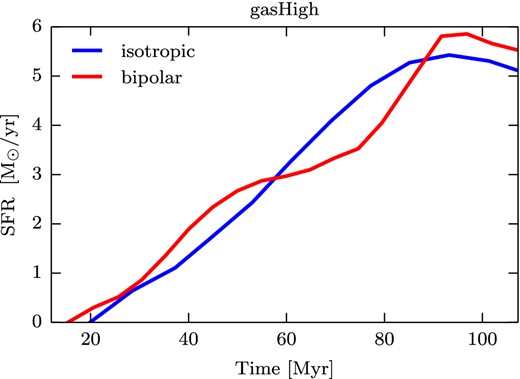
SFR as a function of time: in blue for the case where the pressure is applied isotropically (isotropic) and in red when the pressure is applied to the galaxy in a bipolar geometry (bipolar).
APPENDIX B: EFFECTS OF SUPERNOVA FEEDBACK
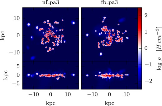
Here, we compare the feedback run with the no-feedback run. In Fig. B1, the gas density maps of the no-pressure enhancement simulations are shown for the no-feedback (nf, left-hand panel) and feedback (fb, right-hand panel) simulations. In Fig. B2, the comparison between fb and nf is shown for the pa3 simulations. We see that for the no-pressure simulations, the effect of SN explosions is to disrupt the ISM into smaller but more numerous clumps. In the edge-on-view, we can also see that the feedback simulation thickens the disc and enhances the mass outflow close to the galaxy. For the pressure simulation, no significant difference can be observed. It shows that the effect of external pressure is stronger than the effect of SN explosions.
In Fig. B3, we show the number of clumps as a function of time for a selection of the gasLow (left), gasHigh (middle), and gasHigh_d (right) simulations with (fb) or without (nf) SN feedback. In Fig. B4, we show the time evolution of the SFR for the same selection of runs. We see that the number of clumps is enhanced by the presence of SN explosions in all cases since the clumps are regularly destroyed by the SN activity (Dubois et al. 2015). SNe regulate the mass growth of the gas clumps, and since the most massive clumps are expected to capture the smaller clumps, SNe allow for the increase in the number of clumps, thereby reducing their average cross-section and mass (see Fig. 7). We also see that the SFR is higher for the no-feedback simulation compared to the feedback simulations as a consequence of the absence of a local regulating process within gas clumps.

Gas density maps (mass-weighted) of the gasHigh non-feedback (left) and feedback (right) simulations without enhancement of the external pressure (nP). The maps are taken at the end of the simulation (∼400 Myr). Each panel shows both face-on (40 × 40 kpc, upper part) and edge-on (40 × 20 kpc, lower part) views.
Similar as Fig. B1 but for the simulations with pressure enhancement pa3.
Time evolution of the number of clumps for a selection of the gasLow (left), gasHigh (middle), and gasHigh_d (right) gasHigh simulations. For each simulation set, the feedback (fb) and no-feedback (nf) runs are shown for comparison. They are indicated by the suffixes in the legend. The lines are smoothed as in Fig. 5.
Time evolution of SFR for a selection of the gasLow (left), gasHigh (middle), and gasHigh_d (right) simulations. For each simulation set, the feedback (fb) and no-feedback (nf) runs are shown for comparison. They are indicated by suffixes in the legend. The lines are smoothed as in Fig. 5.
Reassuringly, the effect of overpressurization of the disc on to the SFR enhancement is independent of the presence of SN explosions: it still leads to a positive feedback effect that SNe only marginally modulate.
APPENDIX C: CONVERGENCE STUDIES
In this section, we test how the results depend on the resolution of the simulation. We performed two highRes simulations for the gasHigh case, one with no external pressure (nP_hR) and the other with external pressure (pa3_hR). The higher resolution runs have been performed with a resolution of Δx = 10 kpc (compared to 40 kpc for the standard runs). We changed the density threshold for star formation (n0 = 224 H cm− 3) in the polytropic EoS as well as the dissipation time-scale of the non-thermal component for the SN feedback (Δx = 10 pc) with the resolution. The simulations were run for a similar time-scale ( ∼ 400 Myr) as the lower resolution (lowRes) simulations.
In Fig. C1, we show the comparison between the highRes and lowRes simulations. In the upper panel, the number of clumps is shown for the highRes and lowRes runs where for both simulations the same clump detection density threshold of 21 H cm− 3 and a peak-to-saddle threshold of 1.5 was chosen.
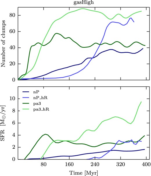
Time evolution of the number of clumps (upper panel) and SFR (lower panel) for the lowRes and highResgasHigh_fb simulations. The clumps were extracted using a gas density threshold of 21 H cm− 3.
Fig. C1 shows that, in both highRes and lowRes runs, clumps are formed at a faster rate when overpressure is applied on the galaxy. Comparing the two resolution runs, we see that the rates of clump formation for both resolutions are comparable at the start of the simulations, for both the pressure and no-pressure runs. While the lowRes run with external pressure (pa3) sees a sharp rise in its clump number at 25 Myr, the number of clumps in the highRes run with external pressure (pa3_hR) starts catching up after 50 Myr and soon (at 70 Myr) overtakes that of the pa3 run, to end up with nearly double the number of clumps. A similar effect is seen in the no-pressure runs: the number of clumps in the highRes simulation starts slowly, but overtakes that of the lowRes run (at 230 Myr) to also end up with nearly double the number of clumps.
Similar trends are seen in the star formation histories (lower panel of Fig. C1). For the no-pressure runs, the highRes one overtakes the other one in SFR at 280 Myr to end up with twice the SFR, while in the corresponding runs with external pressure, the highRes one has its SFR overtake that of the lowRes analogue at 150 Myr, end the highRes run ends up with over double the SFR of the lowRes one. The very slow rise of the SFRs in the highRes runs is the consequence of our choice of a higher density threshold for the highRes simulations, which is reached at later times. Once stars start to form, the SFR is greater in the pressure simulation than in the no-pressure simulation. The general effect that the pressurization leads to more star formation is therefore still the same.
