


Abstract
We present a catalogue of starless and protostellar clumps associated with infrared dark clouds (IRDCs) in a 40° wide region of the inner Galactic plane (|b| ≤ 1°). We have extracted the far-infrared (FIR) counterparts of 3493 IRDCs with known distance in the Galactic longitude range 15° ≤ l ≤ 55° and searched for the young clumps using Herschel infrared Galactic plane survey, the survey of the Galactic plane carried out with the Herschel satellite. Each clump is identified as a compact source detected at 160, 250 and 350 μm. The clumps have been classified as protostellar or starless, based on their emission (or lack of emission) at 70 μm. We identify 1723 clumps, 1056 (61 per cent) of which are protostellar and 667 (39 per cent) starless. These clumps are found within 764 different IRDCs, 375 (49 per cent) of which are only associated with protostellar clumps, 178 (23 per cent) only with starless clumps, and 211 (28 per cent) with both categories of clumps. The clumps have a median mass of ∼250 M⊙ and range up to >104 M⊙ in mass and up to 105 L⊙ in luminosity. The mass–radius distribution shows that almost 30 per cent of the starless clumps identified in this survey could form high-mass stars; however these massive clumps are confined in only ≃4 per cent of the IRDCs. Assuming a minimum mass surface density threshold for the formation of high-mass stars, the comparison of the numbers of massive starless clumps and those already containing embedded sources suggests an upper limit lifetime for the starless phase of ∼105 yr for clumps with a mass M > 500 M⊙.
1 INTRODUCTION
The star formation process begins in massive clouds with a reservoir of gas and dust sufficient to sustain the creation of a cluster of stars (e.g. Lada & Lada 2003), which in some clouds may eventually form high-mass stellar objects (e.g. Rathborne, Jackson & Simon 2006; Peretto & Fuller 2009, hereafter Paper I). Some of these dense, cold clouds which are not yet dominated by star formation absorb the IR emission of the background radiation and therefore can be observed as dark structures in the mid-IR images (infrared dark clouds, IRDCs; e.g. Simon et al. 2006). These relatively undisturbed clouds are favoured places to study the very early stages of star formation (Peretto & Fuller 2010; Battersby et al. 2011; Ragan et al. 2012; Paper I).
Within these clouds, the earliest stages are initially characterized by the formation of a starless, dense clump with a size of ≃1 pc. The cold dust envelope of these clumps emits in the far-IR (FIR)/sub-mm region of the spectrum, but are still IR-quiet at wavelengths ≤70 μm (Elia et al. 2010; Motte et al. 2010; Giannini et al. 2012). As a protostellar core and then protostar eventually forms within the gravitationally bound starless clumps (the pre-stellar clumps) it heats the surrounding envelope. The now protostellar clump becomes visible at wavelengths ≤70 μm and its bolometric luminosity increases, sustained by the warm inner core(s). As a consequence, the protostellar luminosity correlates well with the clump emission observed at 70 μm (Dunham et al. 2008).
Large surveys of the Galactic plane in the FIR-sub-mm region allow us to make a census of these clumps and the young stellar objects (YSOs) within them across the Galaxy. Such surveys provide the significant samples of sources required to understand the star formation mechanisms across a wide range of mass and luminosity regimes as well as identify rare and/or short-lived classes of objects. Several surveys have been carried out in the past few years at increasing sensitivity and spatial resolution in order to build a statistically significant sample of YSOs in the Galactic plane. The APEX Telescope Large Area Survey of the Galaxy (ATLASGAL; Schuller et al. 2009) and the Bolocam Galactic Plane Survey (BGPS; Aguirre et al. 2011) have mapped the inner Galactic plane in the sub-mm range, at 870 μm and 1.1 mm, respectively, allowing a census of the sub-mm thermal emission from high-mass regions. However, unprecedented opportunities to make a multi-wavelength FIR/sub-mm study of the sky arrived with the Herschel satellite (Pilbratt et al. 2010), opening a new window of our understanding of the cold Universe and, in this context, Galactic star formation. For example, the earliest phases of star formation associated with IRDCs have been studied with the EPoS Herschel key programme, for both low-mass (Launhardt et al. 2013) and high-mass objects (Ragan et al. 2012). This survey studied a sample of 12 low-mass and 45 high-mass regions, respectively, in order to characterize the temperature and column densities of the cores and clumps at different mass regimes.
A comprehensive Herschel mapping of the Galactic cold and dusty regions has been recently completed with the Herschel infrared Galactic plane survey (Hi-GAL; Molinari et al. 2010b), which has mapped the whole Galactic plane at latitudes |b| ≤ 1° and following the Galactic warp in the wavelength range 70 ≤ λ ≤ 500 μm.
The aim of this work is to produce a first extensive catalogue of young clumps embedded in IRDCs combining the Hi-GAL data with the most comprehensive catalogue of IRDCs to date (Paper I). This initial catalogue looks in a specific region of the inner Galactic plane, in the longitude range 15° ≤ l ≤ 55°, which encompasses ≃3500 IRDCs with known distance.
The paper is structured as: Section 2 describes the IRDCs data set extracted from Paper I and the Hi-GAL data used to extract the FIR/sub-mm IRDCs counterparts; the source extraction and the catalogues generation are described in Section 3. In this section we also briefly describe Hyper, a new algorithm used in this work and developed for source extraction and photometry in complex backgrounds and crowded fields (Traficante et al. 2015). In Section 4 we describe the statistical distributions of the starless and protostellar clumps properties. Finally, in Section 5 we draw up our conclusions about this first release of clumps in IRDCs.
2 IRDC DATA SET
The IRDCs survey produced in Paper I contains ≃11000 IRDCs identified in absorption against the warm background in the GLIMPSE 8 μm survey of the Galactic plane (Benjamin et al. 2003) delimited by |l| ≤ 65°, |b| ≤ 1°. The IRDCs have been identified as connected regions with column density higher than NH2 ≥ 1 × 1022 cm−2 and a diameter greater than 4 arcsec (Paper I).
We focused on a subsample of 3659 IRDCs observed in the region 15° ≤ l ≤ 55°, |b| ≤ 1°. This region has been selected for its overlap with the Galactic Ring Survey (GRS; Jackson et al. 2006). The GRS emission along the IRDCs line of sight (LOS) has been used to identify clouds and to estimate the IRDCs kinematic distances. The GRS survey mapped the 13CO J = 1–0 emission with the FCRAO 14-m telescope with an angular resolution of 46 arcsec and a spectral resolution of 0.212 km s−1 (Jackson et al. 2006). To obtain kinematic distances, we developed an automated procedure that extracts the 13CO spectrum towards the centre of each IRDC, identifies the number of velocity components in it, integrates each component in a 2 km s−1 interval around the central velocity, and then calculates the ratio map for each of the integrated intensity maps with the Herschel column density, smoothed at 46 arcsec resolution, centred at the IRDC position. We then select the velocity component for which the ratio map is the flattest, i.e. with a minimum dispersion. In some cases, no 13CO(1–0) components were found, and a −999 flag was returned for the velocity. We identified 166 clouds with a −999 flag, therefore our starting IRDC catalogue is composed of 3493 clouds. This procedure is simple, and rather easy to implement for such a large number of sources. Kinematical distances were then calculated using the Reid et al. (2009) Galactic rotation model, always assuming the clouds located at the near distance in case of a distance ambiguity.
2.1 IRDCs Hi-GAL counterparts
The Hi-GAL survey (Molinari et al. 2010b) has been carried out using both the PACS (Poglitsch et al. 2010) and SPIRE (Griffin et al. 2010) photometry instruments on-board Herschel (Pilbratt et al. 2010) in parallel mode, observing the sky at five wavelengths simultaneously (70 and 160 μm with PACS and 250, 350 and 500 μm with SPIRE). The maps have been reduced with the ROMAGAL pipeline (Traficante et al. 2011), an enhanced version of the standard Herschel pipeline specifically designed for Hi-GAL. A weighted post-processing on the maps has been applied to help with image artefact removal (Piazzo et al. 2011). The maps have been flux calibrated (by means of an offset subtraction) following the prescription of Bernard et al. (2010) and are expressed in MJy/sr. Due to the fast scan-speed and the co-addition on-board Herschel of eight samples at 70 μm and four samples at 160 μm, the measured PACS beams in the maps are slightly larger than the nominal ones. The Hi-GAL beams measured on the maps are 10.2 arcsec, 13.55 arcsec, 18.0 arcsec, 24.0 arcsec and 34.5 arcsec at 70, 160, 250, 350 and 500 μm, respectively. The map pixel size is 3.2 arcsec, 4.5 arcsec, 6.0 arcsec, 8.0 arcsec, 11.5 arcsec at 70, 160, 250, 350 and 500 μm, respectively (Traficante et al. 2011).
For each IRDC in our sample we selected the corresponding region in the Hi-GAL 70, 160, 250 and 350 μm maps. We do not include the 500 μm maps in the analysis due to the poor beam resolution compared to the other wavelengths.
Some of the IRDCs of our sample have been already identified in the Hi-GAL survey by Peretto et al. (2010). In this work the authors showed that the IRDC FIR extension is slightly bigger than their appearance at 8 and 24 μm. Therefore, for each IRDC, we isolate an Hi-GAL region which enlarged the 24 μm IRDC size by the equivalent of a 70 μm beam (10.2 arcsec) in each spatial direction. We assume that all the sources extracted between these extended boundaries belong at the same IRDC. Due to the boundaries extension and the proximity of some IRDCs, some sources can be associated with two different clouds. In these cases we associate each source with one IRDC randomly selected from the two clouds.
3 CLUMP EXTRACTION AND PHOTOMETRY
Source extraction and photometry is a well-known problem in astronomy, in particular in complex fields such as the Galactic plane. The high resolution and sensitivity of the new IR instruments have shown the complexity of the sites in which the newly born stars are located (such as the filamentary structures; e.g. Molinari et al. 2010a). In particular, the background variability can be significant in FIR Galactic plane data, especially at longer wavelengths (e.g. Molinari et al. 2010a; Peretto et al. 2010), and models must account for its high variations across each source. Furthermore the Galactic plane is dense and crowded and it is often the case that sources are partially blended together. The problem is further complicated in case of multi-wavelengths study since each band has a different spatial resolution and often single sources are resolved in multiple objects in the high-resolution maps.
Various approaches based on different techniques [e.g. Cutex, Molinari et al. (2011); getsources, Men'shchikov et al. (2012)] have been developed specifically for the new Herschel FIR data, in particular for the Galactic surveys. Cutex in particular is the standard source extraction algorithm used by the Hi-GAL team. It identifies the compact source in the second derivative image of the sky, and fits the sources with a 2D-Gaussian model. In this approach the physical source diameter, FWHMdec, also needed to constraint the source flux, is evaluated through the deconvolution of the HPBW with the FWHMλ of the source measured at each band and it is therefore wavelength-dependent (e.g. Elia et al. 2010; Molinari et al. 2011; Veneziani et al. 2013).
We decide to adopt a different approach and to estimate the flux consistently within the same volume of gas and dust at all wavelengths regardless of the different spatial resolutions. A similar approach has been adopted by Olmi et al. (2013) to study the ClMF in Hi-GAL fields.
For this purpose we used a new algorithm, Hyper (HYbrid Photometry and Extraction Routine), fully described in Traficante et al. (2015). It has been designed specifically to take into account the complexities generated by the new data sets such as the Galactic plane observations made with Herschel, in particular the high background variability and the source crowding. Hyper is based on a hybrid approach between the classical aperture photometry and a 2D-Gaussian modelling of the sources. In the case of multi-wavelength analysis, the region of integration is defined at a particular wavelength and the same region of the sky is used to integrate the flux at all wavelengths. In the following sections, along with the main results of this work we will describe the Hyper parameters tuned for this source extraction and photometry.
3.1 The source catalogues
The sources are initially identified at each wavelength separately on a modified high-pass filtered map using in sequence the find and gcnrtd IDL routines (Traficante et al. 2015). These routines fit a Gaussian model to recognize the peaks above a given threshold σt, defined as a multiple of the rms of the filtered map, σf. A reference threshold value for each Herschel wavelength, which minimizes the false positives and maximizes the identification of real sources, is provided in Traficante et al. (2015). However the source recovery for a given value of σt depends on variations of the (local) background, the source crowding and the cloud size, which differ from cloud to cloud (see also the discussion in Section 4.1.1). We tested several values of σt around the reference values discussed in Traficante et al. (2015) and after visual inspections of randomly selected IRDCs we set σt = [6.0,5.0,4.0,4.0]· σf at [70,160,250,350] μm, respectively. These thresholds are a conservative compromise between source recovery and false identifications. From our visual inspections, less than 1 per cent of the sources appear as false positives. The completeness of our catalogue based on this extraction is discussed in Section 4.1.1.
From this extraction we produced a catalogue of sources independently identified at each wavelength. Hyper identified 8220, 5393, 4967, 3413 sources at 70, 160, 250 and 350 μm, respectively. They are associated with 2070, 1640, 1621, 1246 IRDCs, respectively ≃59 per cent, ≃47 per cent, ≃46 per cent and ≃36 per cent of the whole sample. The high number of 70 μm sources compared to the other wavelengths is likely due to the high spatial resolution of the 70 μm data, which allows the resolution of close sources possibly unresolved at longer wavelengths. Conversely, the low spatial resolution of the 350 μm band blends sources resolved at shorter wavelengths. The longitude distribution of sources at 70, 160 and 350 μm is in Fig. 1. The 250 μm source distribution is very similar to that of the 160 μm sources and is not showed.
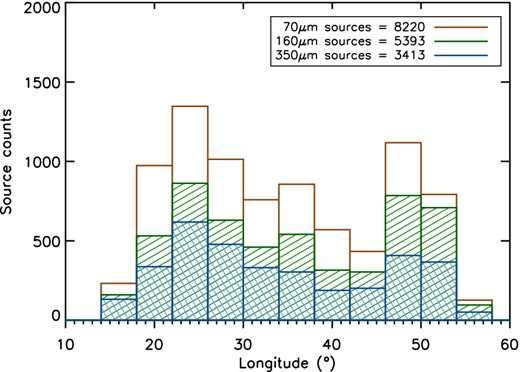
Longitude distribution of sources independently identified at 70 (brown), 160 (green) and 350 (blue) μm. The distribution of 250 μm sources is very similar to the 160 μm distribution and it is therefore not shown.
The multi-wavelength catalogues contain the photometry of the sources observed at all the specified wavelengths, as discussed in the following sections, starting from a reference wavelength used to identify the candidates. The reference wavelength is 160 μm, the highest resolution wavelength that is in common among protostellar and starless clumps. We initially generated a merged catalogue of 160, 250 and 350 μm sources to produce a list of starless and protostellar clump candidates in our selection of IRDCs. At the location of each 160 μm source, a 250 and/or 350 μm counterpart is associated if a source is identified within a radius equal to half the 160 μm beam, 6.7 arcsec. The merged catalogue contains 1723 clumps associated with 764 different IRDCs (≃22 per cent).
A fraction of IRDCs identified in Paper I may not have a counterpart in the Herschel wavelengths and may not be real clouds (e.g. Wilcock et al. 2012); however the small fraction of IRDCs with identified Herschel compact sources here is due to a combination of factors. First, the merged catalogue does not consider sources detected at only one or two wavelengths, nor objects detected at 160, 250 and 350 μm but with centroids separated by more than 6.7 arcsec from the 160 μm centroid. Secondly, most IRDCs smaller than ≃20 arcsec are too small to be associated with a compact Herschel sources. Note that in particular with this choice we are not including in the catalogues the sources observed at 250 and 350 μm with no counterparts at 160 μm. We identified ≃400 sources observed at 250 and 350 μm only. Some of these sources are potentially extremely young, their envelope so cold and/or diffuse that they do not emit above the background at wavelengths λ ≤ 160 μm. However, we cannot extract physical parameters for sources identified at only two wavelengths, therefore we restrict the analysis to the clumps already visible at 160 μm. A multi-wavelength analysis of these very cold clumps is the subject of a subsequent work.
An independent extraction run used to produce a list of 70 μm sources has been combined with the previous sample to produce two final catalogues:
Sources identified at 160, 250 and 350 μm but without counterparts at 70 μm. These sources are classified as starless clumps. The catalogue contains 667 clumps associated with 389 IRDCs. The IRDCs and source longitude distributions are shown in Figs 2 and 3, respectively.
Sources identified at 160, 250 and 350 μm with (at least) one counterpart at 70 μm. A 70 μm source is associated with each clump if its distance from the centroid of the 160 μm source is less or equal to half the 160 μm beam, 6.7 arcsec. These sources are classified as protostellar clumps. This catalogue contains 1056 sources associated with 586 IRDCs. The IRDC and source longitude distributions are shown in Figs 4 and 5, respectively.
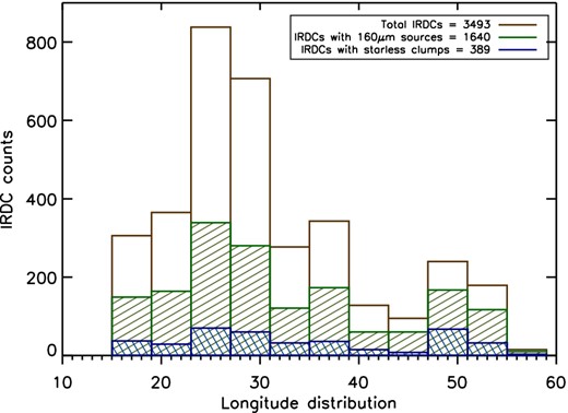
Longitude distribution in the range 15° ≤ l ≤ 55° of IRDCs with at least one starless clump (389, blue) together with the distribution of the IRDCs with at least one 160 μm detection (1640, green) and the distribution of the total number of IRDCs in our catalogue with known distances (3493, brown).
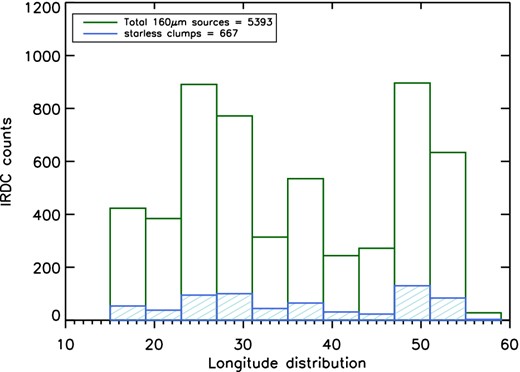
Longitude distribution of sources. In green the 160 μm sources (5393) and in azure the starless clumps (667).
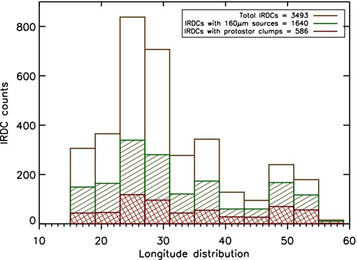
IRDCs longitude distribution of IRDCs with at least one protostellar clump (586, red). The other bars are as shown in Fig. 2.
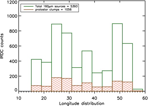
Longitude distribution of protostellar clumps in light red (1056). The other bar is as shown in Fig. 3.
In total, 211 clouds (≃6 per cent of the total) contain both starless and protostellar clumps.
Figs 1–5 show that the majority of the sources are located in the longitude range 25° ≤ l ≤ 30°, and a second peak in the source distribution occurs around l = 50°, for both starless and protostellar clumps. The longitude distribution of the clumps as a function of their distance is shown in Fig. 6. The clump distances are assumed equal to the distance of their parent IRDCs. The median distances are d = 4.2 kpc for both the starless and protostellar clumps.
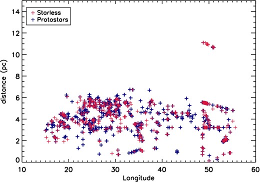
Starless and protostellar clump longitude distribution as a function of their parent IRDC distance. The two distributions look similar and there are no regions with a clear predominance of starless or protostellar clumps. The majority of the sources are located around 25° ≤ l ≤ 30° and l = 50°. The median distances of the two distributions are d = 4.21 kpc and d = 4.23 kpc for starless and protostellar clumps, respectively.
The distribution of clumps is sparse across the Galaxy with two LOS which contain the majority of the clumps and of the 160 μm sources. The region around 25° ≤ l ≤ 30° corresponds to sources mostly located at a distance d ≃ 5 kpc, which is where the LOS passes the tangent point across the Scutum-Crux arm [following the Russeil (2003) spiral Galaxy model]. Being close to the tangent point, the distance ambiguity is minimal for these sources and there are likely to be associated with the Scutum-Crux arm. The source distribution along this LOS is not dominated by starless or protostellar clumps. The peak around l = 50° corresponds to the tangent point of the Sagittarius-Carina arm, but passes also through the Perseus and the Norma-Cygnus arms. Some of the clumps in this region come from the furthest IRDCs present in our catalogue (see Fig. 6), located at ∼10 kpc and are likely to be associated with the Perseus arm. The peak at l = 50° in the source distribution is more evident in the starless clumps. Although some 70 μm sources could be too faint to be observed in the furthest clouds, the mean IRDCs distance around l = 50° is similar to the mean distance of the clouds around l = 30°, 5 kpc and 4.6 kpc respectively. Therefore, the peak at l = 50° in the starless distribution is likely to be a sign of younger star-forming region along this LOS compared to the Scutum-Crux region. The distribution in Fig. 6 indicates that the Hi-GAL sources are mainly located on the Galactic arms, although some are in interarms regions, as already noted by Russeil et al. (2011).
3.2 Photometry
The flux of each source is estimated by integrating the emission within the same elliptical region at all wavelengths. The semi-axes a and b of the elliptical aperture are equal to the FWHMG of the 2D-Gaussian fit to each source estimated at a reference wavelength, which can be different from the wavelength used to initially identify the clumps (Traficante et al. 2015). For the analysis here we set the reference wavelength to λ = 250 μm. The FWHMG of each fit can vary from a minimum of 1 · FWHMλ (18 arcsec at λ = 250 μm) up to 2 · FWHMλ (36 arcsec). This size at λ = 250 μm encompasses a region of at least 1.5 · FWHMλ at λ = 350 μm within the integration area. The range of allowed FWHMG has been chosen in order to account for point-like and slightly elongated compact sources and, at the same time, to avoid highly elongated fits likely contaminated by the underlying filaments aligned with some of the sources. The profile at λ = 250 μm also defines the source size as described in Section 4.1.
We note that within each elliptical aperture the clump could be resolved in multiple objects at 70 and 160 μm. In these cases, the closest source in the cluster is identified as the counterpart and we assign each clump the 70 and 160, μm flux arising from all the sources within the elliptical integration area. This choice is consistent with our approach of evaluating the flux within the same area, since the sources are blended within the beam at longer wavelengths and they all contribute to the observed emission. In the case of these resolved clusters, a specific keyword in the catalogue (‘cluster’) indicates the number of multiple sources observed at 70 and 160 μm within each integration area.
The source flux evaluation is done at each wavelength after the background emission is subtracted and, in case of blended sources, the flux arising from the companions is removed. Hyper evaluates the local background by selecting various square regions across each source and modelling the emission in each region with polynomial functions of different orders (from the zeroth up to the fourth). The fit which produces the lowest rms of the residuals is assumed as best fit and subtracted as background contribution.
Two (or more) sources are considered blended if their centroids are closer than a fixed distance. This distance is automatically evaluated by the algorithm and it is equal to twice the maximum allowed FWHMG (e.g. 72 arcsec), the maximum distance at which two elliptical apertures can be partially overlapped. Each source and its blended companions are fitted simultaneously with a multi-Gaussian function using the mpfit IDL routine (Markwardt 2009). The parameters of the fit are used to build 2D-Gaussian models of the companions which are then subtracted from the image. The flux of the companion-subtracted source is then evaluated as in the isolated source case. A detailed description of the background subtraction and source de-blending strategies can be found in Traficante et al. (2015). However the source fluxes still require to be corrected for two factors: the aperture and colour corrections.
3.2.1 Aperture corrections
Aperture corrections Ac are needed in aperture photometry to compensate for the flux distributed outside the integration area due to the convolution of the true sky signal with the instrumental beam, the PSF response. These corrections therefore depend on the beam at each different wavelength and, for point-like sources, can be estimated by measuring the source emission of reference sources with known flux. A further correction factor has to be applied for extended sources.
For PACS, the aperture corrections are known for circular apertures as function of aperture radius.1 The equivalent aperture radius req of each source, described in Section 4.1, is used to estimate the corresponding Ac.
For SPIRE, aperture corrections are known for circular apertures as function of aperture radius and source spectral index.2 The corrections are estimated at fixed aperture radii of 22 arcsec, 30 arcsec and 40 arcsec at 250, 350 and 500 μm, respectively. Our aperture radius depends on the 2D-Gaussian fit at λ = 250 μm to each source and it is fixed at each wavelength (Section 3.2). However, the range of allowed FWHMG is from 18 to 36 arcsec, therefore we decided to adopt the proposed corrections without further assumptions and assuming a spectral index of β = 2.0 (as discussed in Section 4).
3.2.2 Colour corrections
Colour corrections are needed to convert the flux density measured by PACS and SPIRE into the monochromatic flux density for each observed object, which depends on the intrinsic temperature and spectral energy distribution (SED) of the source. The colour corrections are available online for both PACS3 and SPIRE4 instruments. The colour corrections have been measured for different spectral indexes and blackbody (and greybody) temperatures for both PACS and SPIRE instruments. We adopted a fixed spectral index β = 2.0 (see Section 4). The PACS colour correction curves extrapolated for temperatures in the range 10 ≤ T ≤ 30 K for both the PACS 70 and 160 μm filters are shown in Fig. 7. In order to extrapolate the colour corrections for our sample, however, we need to know the greybody temperature in advance and this poses a circular problem (Pezzuto et al. 2012). So, we estimate the colour corrections following an iterative procedure. We first fixed the colour corrections assuming T = 15 K for both starless and protostellar clumps, in agreement with previous estimations of their envelope temperature (e.g. Veneziani et al. 2013). We obtained a first estimation of the greybody temperatures of our sources resulting in median temperature values of T = 14.37 K and T = 15.84 K for starless and protostellar clumps, respectively. These new values were then used to estimate the first iteration of the colour corrections from the curve in Fig. 7. The SEDs obtained with these new corrections give median temperature values of T = 15.52 K and 17.17 K for starless and protostellar clumps, respectively. Adopting the colour corrections for these temperatures resulted in median temperatures of T = 15.49 K and T = 17.13 K for starless and protostellar clumps, respectively, sufficiently close to the previous estimate, that no further iterate was carried out. The adopted colour corrections are 1.307 and 0.946 for starless and 1.223 and 0.955 for protostellar clumps at 70 and 160 μm, respectively. The SPIRE colour corrections do not vary significantly in the range 10–20 K at β = 2.0. Therefore, we adopted the publicly available values assuming T = 15 K for both starless and protostellar clumps. The values are 1.223 and 0.955 for the 250 and 350 μm fluxes, respectively.
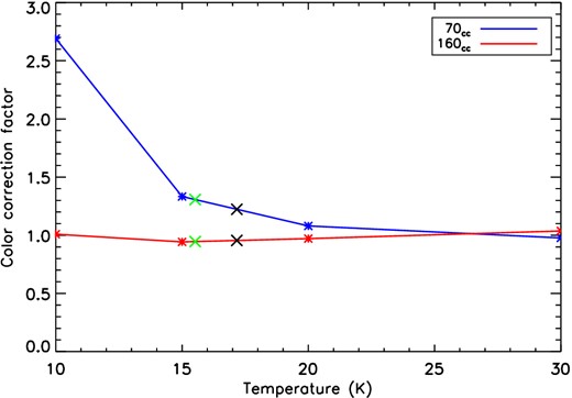
PACS colour correction curves for both the 70 and 160 μm filters, extrapolated from the colour correction values at T = 10, 15, 20 and 30 K described in the PICC-ME-TN-038 PACS report. The green and black crosses show the colour corrections applied for the starless and protostellar clumps flux distributions, respectively. Their values are 1.307 and 0.946 for starless and 1.223 and 0.955 for protostellar clumps at 70 and 160 μm respectively, corresponding to a temperature of T = 15.52 K and 17.17 K for starless and protostellar clumps, respectively.
3.2.3 Flux error
The quoted error for the flux in the PACS and SPIRE reference manuals is, after aperture and colour corrections, <5 per cent. This error has to be combined with the error associated with the Hyper photometry. The error quoted in the catalogues is the flux error estimated as the local sky rms per pixel multiplied for the number of pixels in the area over which the source flux is integrated (Traficante et al. 2015). In addition, the precision in recovering the source flux depends on the intensity of each source and the local background variability. For each source we assume a conservative error of 5 per cent of its flux associated with the aperture and colour corrections plus an error of 15 per cent from Hyper measurements. Hence each source flux has associated a conservative error of 20 per cent of its flux at every wavelength.
3.3 The clumps catalogues
An example of source extraction and photometry at the four considered wavelengths in the SDC23.271-0.263, catalogued as HGL23.271-0.263, is shown in Fig. 8. Hyper identified seven sources observed at 160, 250 and 350 μm simultaneously. Six sources have a 70 μm counterpart and are therefore classified as protostellar clumps, one is classified as starless clump. The 2D-Gaussian fits of the clumps evaluated at 250 μm are shown in green and blue for starless and protostellar clumps, respectively. The sources identified at 160 μm are indicated as black crosses in the 160 μm map.
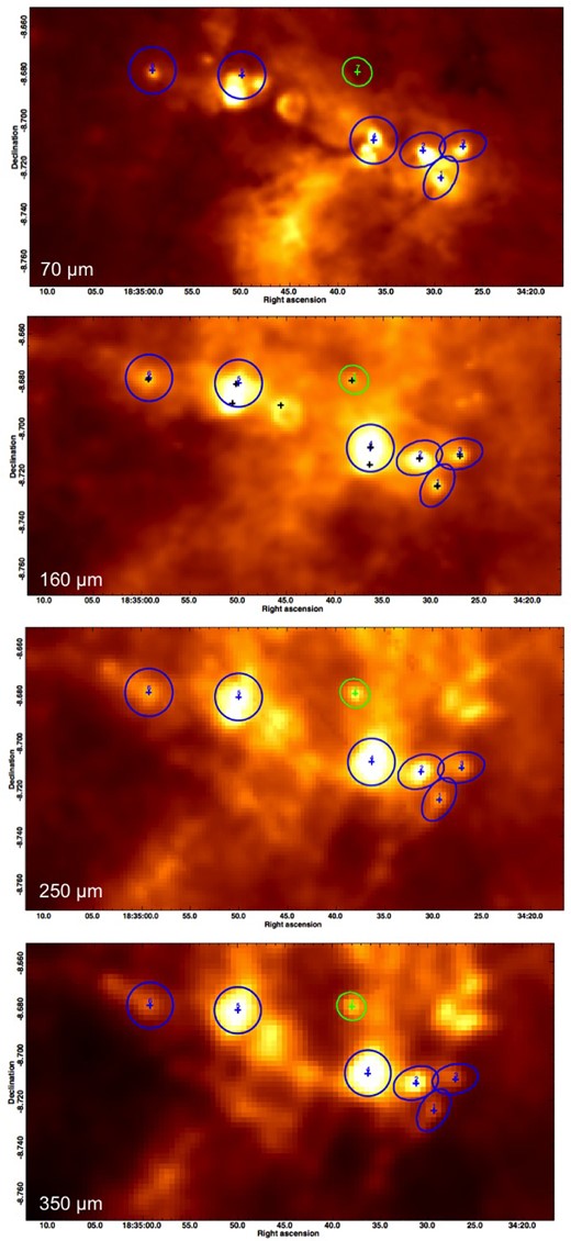
The FIR counterpart of the IRDC catalogued as HGL23.271-0.263. From top to the bottom: 70, 160, 250 and 350 μm images. The protostellar clumps are shown in blue and the starless clumps are shown in green. The ellipses correspond to the elliptical region, defined at 250 μm, used to estimate the source fluxes at all wavelengths. The black crosses in the 160 μm image show the sources initially identified in this map.
The catalogue parameters obtained for the sources extracted in HGL23.271-0.263 are listed in Table 1. The quantities reported for each source are: the IRDC name and the source identification number as extracted from Hyper (Columns 1 and 2), which corresponds to the number in the associated region file; the wavelength (Column 3); the source peak flux in MJy/sr and Jy, evaluated at the centroid pixel (Columns 4 and 5); the source-integrated flux (not corrected) and its associated error (Columns 6 and 7); the sky rms before and after the background subtraction (Columns 8 and 9); the polynomial order used to estimate the background (Column 10); the source semi-axes and the position angles as obtained from 2D-Gaussian fitting at the reference wavelength, 250 μm (Columns 11–13); the convergence status of the fit (Column 14). This status is 0 if the fitting routine converges, otherwise it assumes the value −1 if the source fit is too elongated (axes ratio ≥2.5) or −2 if the fitting routine did not converge. In both these cases the code forces the semi-axes to be equal to the average of the minimum and maximum FWHM possible values (i.e. 1.5 · FWHM250 μm); the position of the source centroids at each different wavelength, in both Galactic and Equatorial (J2000) coordinates (Columns 15–18); the distance between the 160 μm centroid and the centroids of the source counterparts at the other wavelengths (Column 19); the number of sources with their 2D-Gaussian profile overlapped and de-blended before the source flux integration (Column 20). The number of multiple sources resolved at wavelengths other than the 250 μm within the integration area (Column 21).
Output parameters for protostellar and starless clumps extracted in HGL23.271-0.263. The catalogues for protostellar (sources 1–6) and starless clumps (source 7) are separated by a blank line in this table. Column 1: IRDC name. Column 2: Hyper source number. Column 3: wavelength. Columns 4 and 5: source peak flux in MJy/sr and Jy. Columns 6 and 7: source-integrated flux and source flux error in Jy. This source flux is not corrected for aperture or colour corrections. The flux error is estimated from the local sky rms multiplied by the number of pixels in the area over which the source flux is integrated. Column 8 and 9: rms of the sky evaluated in the rectangular region used to model the background before and after the background subtraction, respectively. Column 10: polynomial order used to model the background. Columns 11 and 12: minor and maximum FWHM of the 2D-Gaussian fit. Column 13: Source Position Angle. Column 14: goodness of the 2D-Gaussian fit. Status is equal to 0 if the fit has regularly converged. Columns 15–18: source centroids Galactic and Equatorial coordinates (J2000). Column 19: distance from the source centroids in the reference wavelength and the source counterparts at the other wavelengths. Column 20: number of sources identified as companions and de-blended. Column 21: number of source counterparts at each wavelength. It normally is equal to 1 but it can be higher if the source is resolved in more than one counterpart in the high-resolution maps.
| Map | Sou. | Band | Peak fl. | Peak fl. | Flux | err|${\_}$|flux | sky|${\_}$|nob. | Sky | Ord. | FWHM | FWHM | PA | Status | Glon | Glat | RA | Dec | Dist. | Deb. | Clust |
|---|---|---|---|---|---|---|---|---|---|---|---|---|---|---|---|---|---|---|---|---|
| (μm) | (MJy/sr) | (Jy) | (Jy) | (Jy) | (Jy) | (Jy) | (arcsec) | (arcsec) | (°) | (°) | (°) | (°) | (°) | (arcsec) | ||||||
| 23.271-0.263 | 1 | 70 | 2249.96 | 0.54 | 16.60 | 2.21 | 0.213 | 0.142 | 3 | 21.91 | 36.07 | 149.14 | 0 | 23.242 | −0.240 | 278.623 | −8.726 | 3.35 | 2 | 1 |
| 23.271-0.263 | 1 | 160 | 2623.40 | 1.25 | 37.29 | 3.12 | 0.474 | 0.282 | 1 | 21.91 | 36.07 | 149.14 | 0 | 23.243 | −0.239 | 278.623 | −8.725 | 0.00 | 2 | 1 |
| 23.271-0.263 | 1 | 250 | 1102.27 | 0.93 | 24.60 | 4.16 | 0.734 | 0.501 | 1 | 21.91 | 36.07 | 149.14 | 0 | 23.243 | −0.239 | 278.622 | −8.724 | 1.39 | 2 | 1 |
| 23.271-0.263 | 1 | 350 | 435.34 | 0.65 | 14.70 | 5.08 | 0.949 | 0.815 | 1 | 21.91 | 36.07 | 149.14 | 0 | 23.243 | −0.240 | 278.623 | −8.725 | 3.11 | 2 | 1 |
| 23.271-0.263 | 2 | 70 | 12507.02 | 3.01 | 100.25 | 4.41 | 0.297 | 0.265 | 1 | 25.02 | 36.07 | 110.66 | 0 | 23.256 | −0.240 | 278.630 | −8.714 | 2.94 | 2 | 1 |
| 23.271-0.263 | 2 | 160 | 10611.79 | 5.05 | 114.53 | 4.45 | 0.520 | 0.377 | 4 | 25.02 | 36.07 | 110.66 | 0 | 23.257 | −0.240 | 278.630 | −8.713 | 0.00 | 2 | 1 |
| 23.271-0.263 | 2 | 250 | 4201.20 | 3.56 | 95.12 | 9.93 | 1.295 | 1.119 | 1 | 25.02 | 36.07 | 110.66 | 0 | 23.257 | −0.240 | 278.630 | −8.713 | 0.83 | 2 | 1 |
| 23.271-0.263 | 2 | 350 | 1572.63 | 2.37 | 64.42 | 5.86 | 1.031 | 0.881 | 1 | 25.02 | 36.07 | 110.66 | 0 | 23.257 | −0.240 | 278.630 | −8.712 | 1.75 | 2 | 1 |
| 23.271-0.263 | 3 | 70 | 3661.37 | 0.88 | 43.39 | 3.02 | 0.241 | 0.189 | 1 | 23.10 | 36.07 | 102.28 | 0 | 23.250 | −0.225 | 278.613 | −8.712 | 2.16 | 2 | 1 |
| 23.271-0.263 | 3 | 160 | 3240.27 | 1.54 | 70.44 | 4.08 | 0.345 | 0.359 | 1 | 23.10 | 36.07 | 102.28 | 0 | 23.250 | −0.225 | 278.613 | −8.712 | 0.00 | 2 | 1 |
| 23.271-0.263 | 3 | 250 | 1454.45 | 1.23 | 49.61 | 2.31 | 0.399 | 0.271 | 3 | 23.10 | 36.07 | 102.28 | 0 | 23.251 | −0.224 | 278.613 | −8.711 | 2.97 | 2 | 1 |
| 23.271-0.263 | 3 | 350 | 375.82 | 0.56 | 14.01 | 2.41 | 0.546 | 0.376 | 1 | 23.10 | 36.07 | 102.28 | 0 | 23.252 | −0.225 | 278.614 | −8.710 | 8.79 | 2 | 1 |
| 23.271-0.263 | 4 | 70 | 6063.55 | 1.46 | 89.55 | 5.59 | 0.283 | 0.280 | 2 | 36.07 | 36.07 | 252.40 | 0 | 23.271 | −0.256 | 278.651 | −8.707 | 2.39 | 0 | 4 |
| 23.271-0.263 | 4 | 160 | 13647.29 | 6.50 | 394.78 | 10.69 | 0.767 | 0.753 | 4 | 36.07 | 36.07 | 252.40 | 0 | 23.271 | −0.257 | 278.651 | −8.708 | 0.00 | 0 | 2 |
| 23.271-0.263 | 4 | 250 | 7821.71 | 6.62 | 298.13 | 9.59 | 0.945 | 0.900 | 3 | 36.07 | 36.07 | 252.40 | 0 | 23.271 | −0.257 | 278.651 | −8.708 | 1.27 | 0 | 1 |
| 23.271-0.263 | 4 | 350 | 3162.00 | 4.76 | 138.29 | 4.12 | 0.660 | 0.516 | 3 | 36.07 | 36.07 | 252.40 | 0 | 23.271 | −0.256 | 278.651 | −8.708 | 1.46 | 0 | 1 |
| 23.271-0.263 | 5 | 70 | 1848.66 | 0.44 | 132.85 | 7.69 | 0.451 | 0.385 | 1 | 36.07 | 36.07 | 230.89 | 0 | 23.321 | −0.298 | 278.711 | −8.682 | 8.72 | 0 | 2 |
| 23.271-0.263 | 5 | 160 | 4595.00 | 2.19 | 243.37 | 8.49 | 0.756 | 0.597 | 3 | 36.07 | 36.07 | 230.89 | 0 | 23.321 | −0.295 | 278.709 | −8.681 | 0.00 | 0 | 2 |
| 23.271-0.263 | 5 | 250 | 3167.15 | 2.68 | 161.36 | 6.69 | 0.782 | 0.628 | 4 | 36.07 | 36.07 | 230.89 | 0 | 23.321 | −0.294 | 278.708 | −8.681 | 3.63 | 0 | 1 |
| 23.271-0.263 | 5 | 350 | 1553.36 | 2.34 | 93.40 | 4.34 | 0.591 | 0.543 | 1 | 36.07 | 36.07 | 230.89 | 0 | 23.321 | −0.295 | 278.709 | −8.681 | 0.86 | 0 | 1 |
| 23.271-0.263 | 6 | 70 | 1610.35 | 0.39 | 21.64 | 1.18 | 0.084 | 0.059 | 4 | 36.07 | 36.07 | 117.66 | 0 | 23.339 | −0.327 | 278.746 | −8.680 | 4.49 | 0 | 1 |
| 23.271-0.263 | 6 | 160 | 2004.29 | 0.95 | 47.64 | 2.10 | 0.268 | 0.148 | 4 | 36.07 | 36.07 | 117.66 | 0 | 23.340 | −0.327 | 278.747 | −8.679 | 0.00 | 0 | 1 |
| 23.271-0.263 | 6 | 250 | 971.20 | 0.82 | 45.75 | 2.06 | 0.434 | 0.193 | 4 | 36.07 | 36.07 | 117.66 | 0 | 23.340 | −0.327 | 278.747 | −8.679 | 2.17 | 0 | 1 |
| 23.271-0.263 | 6 | 350 | 465.66 | 0.70 | 22.41 | 2.02 | 0.418 | 0.252 | 4 | 36.07 | 36.07 | 117.66 | 0 | 23.341 | −0.328 | 278.748 | −8.678 | 4.99 | 0 | 1 |
| 23.271-0.263 | 7 | 160 | 1392.66 | 0.66 | 13.40 | 1.02 | 0.243 | 0.116 | 1 | 21.17 | 23.21 | 232.83 | 0 | 23.300 | −0.251 | 278.659 | −8.679 | 0.00 | 0 | 1 |
| 23.271-0.263 | 7 | 250 | 1663.01 | 1.41 | 32.07 | 2.93 | 0.449 | 0.447 | 1 | 21.17 | 23.21 | 232.83 | 0 | 23.300 | −0.250 | 278.658 | −8.679 | 3.78 | 0 | 1 |
| 23.271-0.263 | 7 | 350 | 755.46 | 1.14 | 22.97 | 2.34 | 0.439 | 0.476 | 1 | 21.17 | 23.21 | 232.83 | 0 | 23.300 | −0.249 | 278.658 | −8.679 | 5.28 | 0 | 1 |
4 STARLESS AND PROTOSTELLAR CLUMPS ANALYSIS
For both starless and protostellar clumps we used the fluxes at 160, 250 and 350 μm to model the SED and estimate mass and dust temperature. The FIR luminosity is evaluated by integrating the flux in the range 70 ≤ λ ≤ 500 μm. The 500 μm is extrapolated from the SED fit in both the distributions, where the 70 μm flux is extrapolated from the fit for starless clumps and is obtained from the measured flux for protostellar clumps. The 70 μm flux (and that at shorter wavelengths) of the protostellar clumps is partly influenced by the warm core(s) in the centre (e.g. Dunham et al. 2008; Motte et al. 2010). A single-temperature greybody model cannot account for this second, warm component. Therefore, we do not include the 70 μm emission to estimate the protostellar clump dust temperature and mass.
We note that the temperature gradients across the whole IRDCs can be up to ≃10 K (Peretto et al. 2010), but it is negligible across the starless clumps. Furthermore, the differences in the starless clumps mass estimation assuming a single-temperature greybody model or with a detailed radiative transfer model is negligible (Wilcock et al. 2011). At the same time, the central regions of the protostellar clumps partially warmed-up by the central core(s) are not included in the model, therefore the model underestimates the protostellar clumps central temperature. As a consequence of equation (1), the model could overestimate the protostellar masses (see in Section 4.1). The adopted single clump-averaged temperature model is, however, a reasonable approximation to describe the emission arising from the cold, extended dust envelope of both types of objects. A more complete analysis of protostellar properties requires to model at least two different temperature components, using more sophisticated models (e.g. Robitaille et al. 2007) and using shorter wavelengths to constraint the warm component (e.g. Motte et al. 2010).
The best fit for the greybody model is evaluated with a chi-square minimization analysis using the mpfit IDL routine (Markwardt 2009). In order to restrict the analysis to the sources with good temperature, mass and luminosity estimates, only sources with fits with χ2 ≤ 10 are considered further. To further delimit the sample, we excluded few sources with χ2 ≤ 10 but with unrealistic temperature values (T ≥ 40 K), likely a consequence of constraining the SED with only three points. The majority of the sources have good fits however, and the final catalogue contains 649 out of a total of 667 starless clumps and 1030 out of 1056 protostellar clumps.
Fig. 9 shows the SEDs for the starless and protostellar clumps observed in HGL23.271-0.263. The plots for the protostellar clumps also show the emission at 70 μm, which is in excess of the SED fits in all cases. Each SED plot reports the best-fitting parameters, the distance of the source and the value of the χ2. These values are also reported in Table 2.
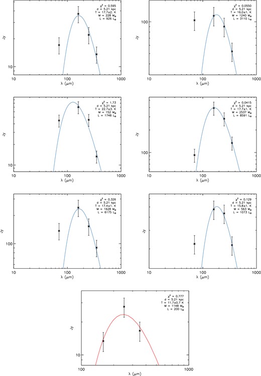
Fluxes at 70, 160, 250 and 350 μm and SEDs for the six protostellar (blue) clumps and the starless (bottom, red) clumps in HGL23.271-0.263. The spectral index is fixed to β = 2.0. The free parameters of the fit are the temperature and the mass, while the luminosity is obtained integrating the emission in the range 70 ≤ λ ≤ 500 μm. The χ2 value of the fit is also shown.
Temperature, mass and luminosity of the seven clumps identified in HGL23.271-0.263, six protostellar and one starless. Columns 1 and 2: IRDC name and source number. Column 3: protostellar or starless type. Columns 4–6: radius, mass and luminosity of each source. Columns 7 and 8: temperature and the associated error estimated with the mpfit routine. Column 9: χ2 value of the greybody fit. Column 10: source distance, equal to the parent IRDC distance.
| IRDC | Source | Type | R | M | L | T | T err | χ2 | Distance |
|---|---|---|---|---|---|---|---|---|---|
| (pc) | (M⊙) | (L⊙) | (K) | (K) | (kpc) | ||||
| 23.271-0.263 | 1 | Protostellar | 0.71 | 228 | 926 | 17.7 | 2.1 | 0.595 | 5.21 |
| 23.271-0.263 | 2 | Protostellar | 0.76 | 1240 | 3110 | 16.0 | 1.6 | 0.055 | 5.21 |
| 23.271-0.263 | 3 | Protostellar | 0.73 | 152 | 1748 | 22.7 | 3.1 | 1.730 | 5.21 |
| 23.271-0.263 | 4 | Protostellar | 0.91 | 2537 | 8591 | 17.7 | 1.9 | 0.042 | 5.21 |
| 23.271-0.263 | 5 | Protostellar | 0.91 | 1628 | 6175 | 17.4 | 1.9 | 0.326 | 5.21 |
| 23.271-0.263 | 6 | Protostellar | 0.91 | 563 | 1073 | 15.8 | 1.5 | 0.129 | 5.21 |
| 23.271-0.263 | 7 | Starless | 0.56 | 1148 | 200 | 11.7 | 0.7 | 0.777 | 5.21 |
4.1 Radius, temperature and mass distributions
We adopt a source size given by the equivalent radius req, defined as the radius of a circle with the same area, |$A=\pi r_{\rm eq}^2$|, as the elliptical region evaluated from the 250 μm source fit. Unlike previous work on Herschel data we do not assume the deconvolved radius to describe the source size, which is a description of the intrinsic shape of the source but it is wavelength-dependent (e.g. Motte et al. 2010; Giannini et al. 2012; Elia et al. 2013). Instead, |$r_{\rm eq}=\sqrt{A / \pi }$| describes the dimension of the region across which the flux is evaluated at all wavelengths.
The distribution of req for both starless and protostellar clumps is shown in Fig. 10. A Kolmogorov–Smirnov (KS) test shows that there is no evidence that the distributions are different. The median values of the two distributions are similar, |$\bar{r}_{\rm eq}\simeq 0.6$| pc. At the median distance of our sample of IRDCs (4.2 kpc; see Section 3.1) the SPIRE 250 μm beam is equivalent to ≃0.4 pc, therefore in most cases we cannot resolve single cores (r ≤ 0.1 pc; Bergin & Tafalla 2007). The apparent size threshold around R ≃ 1 pc is because the vast majority of the sources lie below ≃5.5 kpc and we set the maximum aperture radius, which defines the equivalent radius Req (see Section 4.1), to twice the FWHM250μm, 36 arcsec, which corresponds to Req ≃ 1 pc at d = 5.5 kpc. This choice of restricting the fit to twice the FWHM250μm is made to isolate compact structures embedded in the clouds and we expect the clumps to be relatively circular, with aspect ratios of less than 2 on average (e.g. Urquhart et al. 2014). The few sources with radii req ≥ 1 pc are associated with the furthest IRDCs of our catalogue, located around d ≃ 10 kpc in correspondence of the Perseus arm at l ≃ 50° (see Section 3.1).
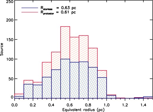
Equivalent radius distribution of the clumps identified in the catalogue for both starless (red) and protostellar (blue) clumps. The mean values are 0.61 pc and 0.63 pc for starless and protostellar clumps, respectively. The radii have been evaluated as the radii of circles with the same area of the ellipses estimated from the 2D-Gaussian fits at 250 μm, as explained in detail in the text.
The distribution of source temperature for both the starless and protostellar clumps is shown in Fig. 11. The median temperatures of the distributions are T ≃ 15.5 K and T ≃ 17.1 K for starless and protostellar clumps, respectively. These temperature distributions are in agreement with similar analysis of starless and protostars done with Hi-GAL both in the inner Galaxy (e.g. Veneziani et al. 2013) and in the outer Galaxy (e.g. Elia et al. 2013). The KS test shows that the probability that the two distributions are the same is <10−9, although it is clear that the protostellar clumps are only slightly warmer than starless clumps on average. Since the emission in the 160–350 μm spectral range arises from the dust envelope for both starless and protostellar clumps, this result implies that the protostellar envelope is only partially warmed-up by the central core(s), which may be an indication of the youth of the protostellar systems.
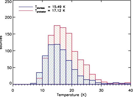
Temperature distribution of the 1723 clumps, starless (red) and protostellar (blue). The median values are T = 15.49 K and T = 17.12 K, respectively, suggesting that the cold dust envelopes are slightly warmed by the central core(s) in the protostellar clumps.
The mass distributions of the sources are shown in Fig. 12. The red vertical line defines Mcom = 105 M⊙ which indicates the mass completeness limit as explained in the next section. This limit lies below the turnover point which is around M ≃ 103 M⊙. The identified sources span a wide range of masses, from few solar masses up to few ≃104 M⊙ with average clump mass of ≃193 M⊙ and ≃272 M⊙ for starless and protostellar clumps, respectively. The distributions are similar for both starless and protostellar dumps, likely due to the fact that the envelope of these clumps is not substantially perturbed by the internal gravitational collapse which is occurring in the protostellar cores (Giannini et al. 2012). Some of these clumps are potentially the birth site of high-mass objects, as discussed in Sections 4.2 and 4.3.
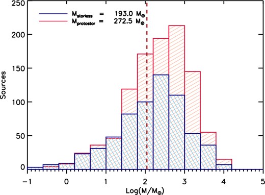
Mass distribution of the 1723 clumps, starless (blue) and protostellar (red). The dashed red line is the mass completeness, fixed at M = 105 M⊙. The mass range spans several order of magnitudes, from few solar masses up to few 104 M⊙. The median values are M = 194 M⊙ and M = 269 M⊙ for starless and protostellar clumps, respectively.
Some of the clumps in the sample have also been observed as part of the Herschel EPOS survey of high-mass star-forming IRDCs by Ragan et al. (2012). They found 496 protostellar cores and clumps simultaneously observed at 70, 100 and 160 μm associated with 45 IRDCs across the Galactic plane. Longer wavelengths were excluded from the analysis in order to preserve the high spatial resolution of the PACS data. In the Ragan et al. (2012) catalogue 64 protostellar clumps fall in the longitude range 15° ≤ l ≤ 55° and overlap with our sample. All these 64 sources were detected in our analysis at 70 μm, but only 35 of them have observable counterparts at 160, 250 and 350 μm and are part of the protostellar clump catalogue. In addition three sources have been identified as starless, since the 160 μm centroids are located more than 6.7 arcsec away from the 70 μm source (Section 3.1).
The properties of the two overlapping samples are not straightforward to compare, since the higher spatial resolution of the Ragan et al. (2012) sample allows them to model the properties of the inner part of the clumps, and in some cases of the single cores. Indeed, in our catalogue the dust temperature are, on average, 5 K colder and the mass are, on average, a factor of ≃8 higher compared to the Ragan et al. (2012) catalogue. The mean mass for the three clumps we identify as starless is M ≃ 2900 M⊙ whereas Ragan et al. (2012) find a mean of M ≃ 740 M⊙. Similarly for the 35 protostellar clumps, in our catalogue the mean mass is M ≃ 1350 M⊙ whereas Ragan et al. (2012) find M ≃ 215 M⊙. The inclusion of the 70 μm flux in the SED fitting by Ragan et al. (2012) significantly raises the temperature estimation which contributes to these mass differences. The sources have a mean temperature of 14.4 and 18.3 K for starless and 17.5 and 21.7 K for protostellar clumps, in our catalogue and in the Ragan et al. (2012) catalogue, respectively.
It is important to note that the mass (and mass surface density) values have significant uncertainties due to the assumed dust model. The opacity and the spectral index of the dust can vary among the different models by a factor of 2 or more (Ormel et al. 2011). High-resolution, multi-wavelength observations at sub-mm/mm wavelengths are required to better constraint the dust properties and hence the mass of each clump.
4.1.1 Mass completeness
The mass completeness of the catalogue is determined by the ability to recover faint sources in the presence of highly variable backgrounds, which vary from cloud to cloud by orders of magnitude. Also, we are extracting sources from thousands of relatively small clouds located at a range of distances, d, which will have masses ∝ d2 (see equation 1). Therefore a single completeness limit for the catalogue is poorly representative of the whole sample of clouds. Instead, a mass completeness needs to be evaluated locally for each cloud which accounts for the background confusion and the source distance.
In order to derive the local mass completeness for each cloud we compared the mean mass of the embedded clumps with the corresponding mean background-equivalent source mass Mbg of each cloud. For each clump we define the background-equivalent source as a point source with a flux equal to the clump background flux integrated in a circular region with a radius equal to the FWHM250 μm at all wavelengths (see Section 3.2). The clump background flux per pixel at each wavelength is defined as the average flux emission per pixel evaluated in a region surrounding each clump, with the clump masked and with a sigma-clipping procedure to avoid significant contamination from companion sources.
The background-equivalent source mass is then evaluated using the same SED fitting procedure described in the previous section and assuming for the background sources the same distance as their corresponding IRDC. The mean value of all the background-equivalent source masses in each cloud determines the local IRDC Mbg.
The mean mass of the background-equivalent sources compared with the sources in each IRDC is shown in Fig. 13. Sources with a mass up to Mbg are hidden in the background emission and unidentifiable in that specific cloud. Mbg sets a local mass completeness limit which accounts for the local background variation and the IRDC distance. There are a few tens of clouds with Mbg ≥ 102 M⊙ and, at the same time, several clouds for which sources with M ≤ 10 M⊙ are easily identifiable. On average the mean source mass is few times greater than the corresponding mean Mbg; however there are identified sources with masses close to the corresponding mean Mbg.
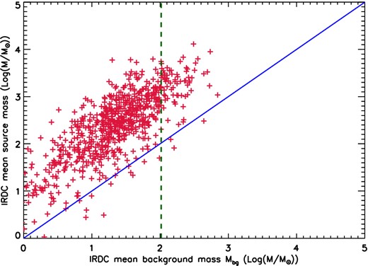
Distribution of the mean source mass per IRDC as a function of the Mbg. The blue line is the y = x line. The majority of the clumps have M ≥ Mbg.
To set an estimate of the mass sensitivity limit for the whole catalogue, we identify the mass value Mcom where 90 per cent of clouds have Mbg≤ Mcom (the green dashed line in Fig. 13). In other words, in 90 per cent of the clouds all sources with masses M > Mcom are detected. This mass value is Mcom ≃ 105 M⊙. We define this value as a mass completeness limit for the catalogues. The remaining 10 per cent of the clouds with Mbg above the limit are among the furthest in the catalogue, with a mean distance of 5.4 kpc (in comparison with the average distance of the whole catalogue, 4.2 kpc; see Section 3.1).
We stress that this mass completeness limit is strongly influenced by the IRDC distance and has to be taken ‘cum grano salis’, in general a local mass completeness should be used for each cloud. As showed in Fig. 14, the distribution of Mbg substantially changes if we divide the source sample in two subsets, one including all the sources located at d ≤ 4.2 kpc and one including all the sources located at d ≥ 4.2 kpc. Mcom(d ≤ 4.2) = 37 M⊙ and Mcom(d ≥ 4.2) = 167 M⊙ for the close and the far sample, respectively. To further demonstrate that the mass completeness is dominated by the diffuse emission and depends on the source distance, we estimated the mass of a background-equivalent source located at the mean distance of d = 4.2 kpc and with an emission at 160 μm arising from residual noise only (0.6 Jy/pixel; Traficante et al. 2011). Its mass is ≃10 M⊙ (the orange-dotted line in Fig. 14). For comparison, the average Mbg of all clouds located at ≃4.2 kpc is ≃30 M⊙, while ≃10 M⊙ is the mean Mbg of clouds located at ≃2.2 kpc.
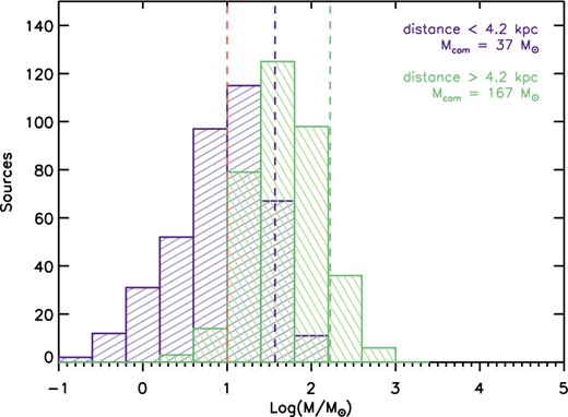
Mbg distribution for sources located at d ≤ 4.2 kpc (purple histogram) and at d ≥ 4.2 kpc (green histogram). Mcom, which defines the mass value above which all sources are identified in 90 per cent of the clouds, changes significantly with distance with values of Mcom = 37 M⊙ for the distribution of the closest sources and Mcom = 167 for the distribution of the more distant sources. The orange-dotted line shows for comparison the mass of a background-equivalent source located at the mean distance of d = 4.2 kpc and with an emission at 160 μm arising from residual noise only.
Finally, we note that the selection criteria of our sample of clouds (see Section 2), together with the local mass completeness discussed in this section, do not produce a complete sample of objects. Mcom gives a reference value which only defines that we recover sources with masses ≥Mcom in 90 per cent of the clouds and it is not related to the underlying intrinsic clump mass spectrum, for which a statistically complete sample would be required. As a consequence, for example, it is not clear whether the turnover point in the source mass distribution, around M ≃ 103 M⊙ (see Fig. 12), is meaningful beyond describing the actual distribution of clumps in the catalogue. The local mass completeness values for each cloud are available with the source catalogues.
4.2 Mass versus radius
In the past it has been suggested that IRDCs are favourable places for high-mass star formation (e.g. Carey et al. 1998). This suggestion has been corroborated by several observations of massive YSOs associated with IRDCs (e.g. Beltrán et al. 2013; Beuther et al. 2013; Peretto et al. 2013). However, IRDCs are also forming low-to-intermediate stars in regions devoid of high-mass stars (e.g. Sakai et al. 2013).
One way to determine if the clumps associated with the IRDCs are ongoing high-mass star formation is to look at the mass–radius distribution under the assumption that, in order to form high-mass stars, a large amount of material needs to be concentrated into a relatively small volume. Recently an empirical threshold for the formation of mass stars in IRDCs has been proposed. This threshold is, in its original formulation, m(r) > 870 M⊙ (r/pc)1.33 (Kauffmann & Pillai 2010, hereafter KP). This model accounts for single fragments within each star-forming region and it is well suited to be compared with our clumps catalogue. In Fig. 15 we show the mass–radius relationship for our catalogue of starless clumps, colour-coded for their dust envelope temperature. The light brown shaded area delimits the KP region above which massive stars can be formed. For comparison, the figure also shows Larson's third law as it appeared in its original formulation, m(r) > 460 M⊙ (r/pc)1.9 (green dashed line), which describes the universality of the scaling relation between mass and radius of molecular clouds (Larson 1981).
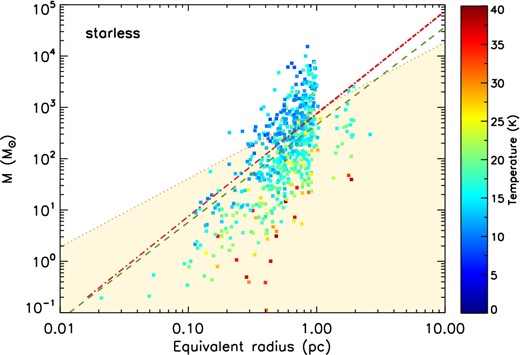
The mass of the starless clumps as a function of their equivalent radius, colour-coded for the temperature of the dust envelope. The mass increases with increasing equivalent radius. The unshaded area delimits the region of the high-mass star formation in IRDCs as determined by the KP empiric analysis. Almost one third of the starless clumps (171 out of 667) lie above this threshold. The line-dotted red line is the threshold adapted from Urquhart et al. (2014) who propose an empirical lower limit value for high-mass star formation equivalent to a constant mass surface density of Σ = 0.05 g cm−2. The green dashed line is the Larson (1981) universal scaling relation between mass and radius of molecular clouds, shown for comparison.
We identify 171 starless clumps above the KP threshold, distributed in 130 IRDCs. Interestingly by this criterion ≃26 per cent of the starless clumps are likely to form high-mass stars. These are situated in ≃33 per cent of the IRDCs with identified starless clumps (389; Section 3.1). At the same time, the clouds which encompass these high-mass starless clumps are only 4 per cent of the total clouds in our sample (3493; see Section 2). While the mass completeness limit influences the percentage of high-mass starless clumps, the number of clouds which embed these high-mass clumps is much less affected since it is unlikely that we are missing the most massive objects associated with the clouds. We can conclude that only a small fraction of IRDCs will potentially form high-mass stars, in agreement with the results of KP.
The dash–dotted red line in Fig. 15 defines the empirical threshold for high-mass star formation proposed by Urquhart et al. (2014). This threshold is based on the analysis of high-mass star-forming clumps identified in the ATLASGAL survey and corresponds to clumps with a constant mass surface density of Σ = 0.05 g cm−2. This threshold, however, sets less stringent constraints than the KP threshold for clumps with an equivalent radius of R ≤ 1 pc, which are the majority of the clumps in our survey. We discuss in the next section the mass surface density thresholds for high-mass star formation compared with our sample.
The mass–radius diagram for protostellar clumps is shown in Fig. 16. A direct comparison of the protostellar clump sample with the KP threshold is less meaningful however, since the mass estimation of protostellar clumps can be affected by mass-loss in jets or outflows, or mass segregated in the central core(s) as well as overestimating the mass as a result of using a single-temperature model and incompletely accounting for the heating by the central protostars. However, we find 456 protostellar clumps (≃43 per cent of the total) associated with 291 IRDCs (≃50 per cent of the IRDCs with embedded protostars, and ≃8 per cent of the total) above the KP threshold and so are capable of forming high-mass stars.
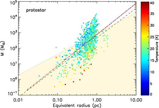
The mass of the protostellar clumps as a function of their equivalent radius, colour-coded for the temperature of the dust envelope. There are ≃43 per cent of the protostellar clumps (456 out of 1056) above the KP threshold.
The low percentage of IRDCs possibly forming high-mass stars does not exclude however that the majority of the high-mass star formation activity is associated with IRDCs. This issue can be addressed, for example, by comparing the star formation activity within the IRDCs and in a large sample of massive molecular clouds not associated with IRDCs, or tracing the star formation rate inside and outside IRDCs. Both these analyses are the main topic of a forthcoming work.
The temperature distribution in the diagrams shows that the colder clumps are the bigger and the more massive. For starless clumps this may be an indication of their evolutionary phase, with the smaller clumps having already started central accretion and likely being just at the verge of a protostar core formation, or maybe with a very young protostar already formed but still obscured at 70 μm. For protostellar clumps this is likely a consequence of the adopted model, since the single clump-averaged temperature is dominated by the extended cold dust envelope emission with less contribution from the warmer central regions as the clump size increases.
4.3 Mass and mass surface density
The environment of massive star formation can be also investigated through the mass surface density, Σ, versus mass diagram. The work of Krumholz & McKee (2008) suggested Σ = 1 g cm−2 as a mass surface density threshold required to prevent fragmentation into low-mass cores as a result of radiative feedback, thus allowing high-mass star formation. However, this threshold has a large scatter and the calculation does not include the contribution of magnetic fields, which can prevent fragmentation without imposing a minimum mass surface density (e.g. Butler & Tan 2012). Several high-mass clumps and cores are indeed observed with 0.1 ≤ Σ ≤ 0.5 g cm−2 (Butler & Tan 2012; Tan et al. 2013). One of the most massive cores observed in the inner Galaxy, associated with the IRDC SDC335, with a mass of ≃500 M⊙ in ≃0.05 pc (Peretto et al. 2013) reaches Σ ≃ 60 g cm−2. However the mass surface density of the embedding clump, with a mass of ≃2600 M⊙ in ≃1.2 pc (Peretto et al. 2013), is Σ ≃ 0.5 g cm−2. The dark cloud, with a mass of ≃5500 M⊙ within ≃2.4 pc, has a mean surface density of Σ ≃ 0.25 g cm−2. On average, high-mass star-forming regions associated with IRDCs are usually observed within 0.1 ≤ Σ ≤ 1 g cm−2 (Tan et al. 2014). As discussed in the previous section, a less stringent empirical threshold for high-mass star formation in clumps has been suggested by Urquhart et al. (2014) based on ATLASGAL clump studies and corresponds to Σ ≥ 0.05 g cm−2.
In Figs 17 and 18 we plot the mass surface density–mass diagrams for the starless and protostellar clumps respectively, colour-coded for the temperature of the dust envelope. The light-brown shaded area delimits the Σ ≥ 0.1 g cm−2 region. There are 144 starless and 308 protostellar clumps, respectively 22 per cent and 29 per cent of the two samples, within this region where massive star formation is possible. Adopting the Urquhart et al. (2014) threshold limit increases these numbers to 241 starless and 542 protostellar clumps (≃36 and ≃51 per cent of the respective samples). Following Tan et al. (2014), we also show straight lines corresponding to constant radius, constant escape speed and constant hydrogen number density. The apparent radius threshold at R ≃ 1 pc is due to our choice of the maximum aperture size of clumps and the distance distributions of clouds, as discussed in Section 4.1.
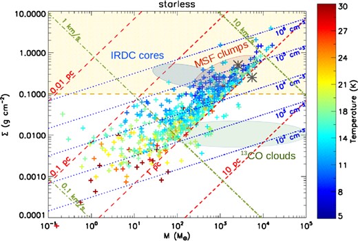
Mass surface density as a function of mass for starless clumps, colour coded for the temperature of the dust envelope. The light brown shaded area defines the region of sources with surface density Σ ≥ 0.1 g cm−2. The lines correspond to constant values of various parameters: red lines: constant radius; blue lines: constant H number density, analogous of constant free-fall time; green lines: constant escape velocity. Also shown are the regions corresponding to IRDC cores observed by Butler & Tan (2012, blue shaded area), the massive star formation clumps (and cores) observed by Mueller et al. (2002, red shaded area) and the 13CO molecular clouds from the catalogue of Roman-Duval et al. (2010, green shaded area). The dark grey asterisks show the location of the SDC335 central clump and cloud (Peretto et al. 2013).

Mass surface density as a function of mass for protostellar clumps, colour coded for the temperature of the dust envelope. The shaded areas and lines are as shown in Fig. 17.
The escape speed is vesc = (10/αvir)1/2σ, with αvir being the virial parameter and σ the velocity dispersion of the clump. Assuming a virial parameter αvir = 1 for gravitationally bounds clumps and an average velocity dispersion of σ = 1 km s−1 (e.g. Henshaw et al. 2013; Kauffmann, Pillai & Goldsmith 2013) the escape speed is vesc ≃ 3 km s−1. Therefore, for a typical high-mass star-forming clump with mass of M ≃ 1000 M⊙ (Tackenberg et al. 2012; Urquhart et al. 2014), the clump is bound if its mass surface density reaches Σ ≃ 0.1 g cm−2. Low values of viral parameters have been observed in region of high-mass star formation (e.g. Li et al. 2013; Tan et al. 2013). Assuming αvir = 0.5 the corresponding escape speed becomes vesc ≃ 4.5 km s−1 and a M ≃ 1000 M⊙ clump will be bound only if it reaches Σ ≃ 0.3 g cm−2 or, equivalently, if its mass is confined in a radius R ≃ 0.45 pc. We find 38 starless and 76 protostellar clumps with Σ ≥ 0.3 g cm−2, ≃ 6 per cent and ≃7 per cent of the two samples, respectively. We find only four starless and four protostellar clumps with Σ ≥ 1 g cm−2.
The hydrogen number density nH is analogous to constant free-fall time, following the relation tff = [3π/(32Gρ)]1/2, where ρ is the volume density of the clump. From the diagram we note that, setting the high-mass star formation threshold at Σ ≥ 0.3 g cm−2, the minimum hydrogen number density of high-mass star-forming clumps is nH = 105 cm−3. This value corresponds to a free-fall time of 1.4 × 10⁵ yr. Assuming as a lower limit for the mass surface density Σ ≥ 0.1 g cm−2 to form high-mass stars, from the diagram we deduce a minimum hydrogen number density of nH ≃ 1.5 × 104 cm−3, or a free-fall time of 3.6 × 10⁵ yr. With the surface density proposed by Urquhart et al. (2014), from our clumps distribution we deduced a minimum hydrogen number density of nH ≃ 8 × 103 cm−3, or a free-fall time of 5.0 × 10⁵ yr.
For comparison we highlighted the regions in the plots occupied by cores/clumps associated with a sample of 10 IRDCs selected by Butler & Tan (2012), the 51 massive star-forming clumps identified by Mueller et al. (2002) and the 13CO molecular clouds identified in Roman-Duval et al. (2010). The SDC335 central clump and cloud values are also shown in the plot with dark grey asterisks.
4.4 Luminosity
Fig. 19 shows the FIR luminosity distributions of the clumps. The median values of the luminosities are L = 83 L⊙ and L = 590 L⊙ for starless and protostellar clumps, respectively. This difference in the FIR luminosity is principally due to the emission arising from the warm core(s) in the protostars. In the starless clumps the luminosity of the dust envelope is the only contribution to the bolometric luminosity. On the other hand, the warm core(s) in the protostellar clumps contributes substantially to the integrated FIR luminosity. Depending on the evolutionary state of a protostar there can also be significant emission at 24 μm or shorter wavelengths. The estimated FIR luminosity is therefore a lower limit of the protostars bolometric luminosity (e.g. Giannini et al. 2012).
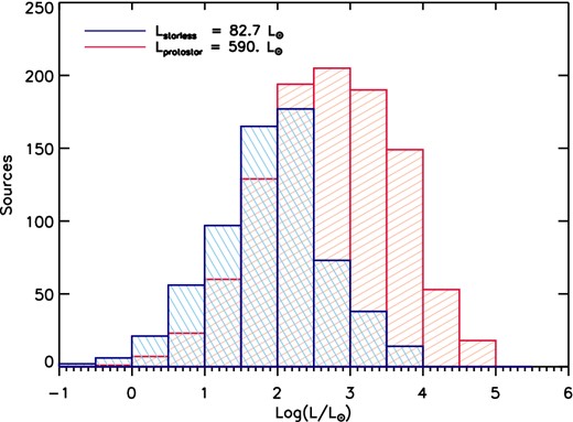
FIR luminosity distributions for the 1723 clumps, evaluated in the range 70 ≤ λ ≤ 500 μm as detailed in the text. The median values are L = 83 L⊙ and L = 590 L⊙ for starless and protostellar clumps, respectively. This difference is a direct consequence of the internal luminosity of the core(s) embedded in the protostellar clumps which are partly visible in the 70 μm emission.
We identified 71 protostellar clumps (≃7 per cent of the total) with L ≥ 104 L⊙. There are 52 starless clumps with L ≥ 103 L⊙, relatively high for starless clumps. The majority of them (30 out of 59) have a bolometric luminosity versus envelope mass (Lbol/Menv) ≤ 1, indicative of objects without warm cores. These are among the most massive starless clumps identified in this catalogue. The remaining 22 starless clumps with luminosity L ≥ 103 L⊙ and Lbol/Menv > 1 are either very young protostellar clumps or not confirmed starless, as from visual inspections some of them show them to be associated with particularly faint 70 μm sources not identified with our selection threshold (see Section 3.1) or associated with bright diffuse 70 μm emission.
4.5 Mass luminosity
A potentially useful tool to infer the evolutionary properties of the young clumps is the Lbol–Menv diagram. This diagram has been successfully used in the past to describe the evolutionary phases of low-mass objects (Saraceno et al. 1996), and subsequently extended to predict the evolutionary paths of high-mass objects (Molinari et al. 2008). A source evolves following specific tracks, depending on its initial mass and luminosity, and the model predicts the mass and luminosity of the object when it reaches the zero age main sequence (ZAMS). For high-mass objects the paths follow the two-phase model of McKee & Tan (2003). According to this model, when a cloud starts its gravitational collapse the mass slightly decreases due the accretion and molecular outflows, while the luminosity of the object increases significantly, sustained by the collapse. The source moves along almost vertical paths in the diagram. At the end of this phase the object is surrounded by an H ii region, the luminosity remains constant while the mass is expelled through radiation and molecular outflows. The object then follows an almost horizontal path, which will end when it becomes visible in the optical and almost all the envelope has been expelled. Accordingly to the evolutionary phase in the diagram, the high-mass objects are classified in analogy with the low-mass regime classification, from Class 0 to Class II prior to the ZAMS phase. This classification can be misleading though, and some caveats of this model have to be kept in mind, in particular when applied to our sample: (1) the transition from Class 0 to Class I and Class II sources in the low-mass regime is not sharp. Sources classified as Class 0 based on their NIR–MIR fluxes can instead be classified as Class I in the FIR (Hennemann et al. 2010; Elia et al. 2013); (2) the evolutionary tracks have been initially modelled for single cores, not for clumps and (3) in high-mass regions the observed clumps can contain multiple cores in different stages of evolution and the clump luminosity is likely dominated by the most evolved core(s). Nevertheless, the Lbol–Menv diagram has been used in the past to discuss the evolutionary tracks of YSOs with Herschel data in a wide range of different conditions, both for low-mass (e.g. Bontemps et al. 2010; Hennemann et al. 2010) and for intermediate-to-high mass regime (e.g. Elia et al. 2010; Veneziani et al. 2013).
The Lbol–Menv diagram for the starless clumps is shown in Fig. 20. The distribution is superimposed to the models of Saraceno et al. (1996) and Molinari et al. (2008), which shows the tracks for stars with final masses of 6.5, 8, 13.5, 18 and 35 M⊙ from left to right, respectively. The best log–log fit for Class I and Class 0 high-mass objects (Molinari et al. 2008) is also shown. The majority of the sources lie below the best log–log fit of Class 0 objects. Also, the distribution lies on average below the distribution of young high-mass clumps identified in Urquhart et al. (2014), which includes clumps at different stages of evolution but does not include starless ones. We find a mean Lbol/Menv ≃ 1.1, compared with a mean Lbol–Menv ≃ 10 of Urquhart et al. (2014), consistent with the majority of these starless clumps being in a very early stage of their evolution. Fig. 21 shows the Lbol–Menv diagram for the protostellar clumps. The distribution overlaps that of the starless clumps, proving little discrimination between the relative evolutionary stages of the sources. However the mean Lbol–Menv ≃ 6.6 is an indication of a more evolved phase and including measurements at shorter wavelengths will increase the luminosity of many sources (Section 4) and raise the distribution in the diagram. In addition, higher angular resolution measurements which can resolve the actual envelope mass (as opposed to the clump mass) associated with each protostar, will move the points to the left. Without these additional data, the high degree of overlap in the distributions limits the value of these plots for probing the evolutionary status of the sources.
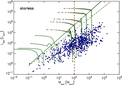
Lbol–Menv diagram for starless clumps superimposed with the model of Saraceno et al. (1996) and Molinari et al. (2008, green lines). The solid and dashed lines are the best log–log fit for Class I and Class 0 sources respectively, extrapolated in the high-mass regime by Molinari et al. (2008). The red vertical line is our mass completeness limit, M = 105 M⊙. The sources are sparse in the diagram but the majority are below the Class 0 fit, showing that they are in a very early stage of evolution.
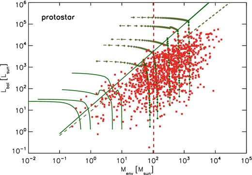
The same diagram as Fig. 20 but for protostellar clumps.
4.6 Clumps lifetime
Comparing the number of starless to protostellar clumps provides an estimate of the lifetime of the starless phase. This is of particular interest for those regions most likely to form high-mass stars, the most massive clumps with high surface densities. For clumps with a mass M > 500 M⊙ and a surface density Σ > 0.1 g cm−2 the ratio of the number of starless clumps to protostellar clumps is 0.46, which increases only slightly to 0.48 when considering clumps with a surface density Σ > 0.3 g cm−2. This suggests a lifetime for the starless phase of about half that of the protostellar phase. Adopting an estimate of few× 105 yr for the lifetime of the embedded phase of young massive stars (e.g. Davies et al. 2011), the starless phase duration would be ∼105 yr, in agreement with the lifetime estimation of starless clumps identified in the ATLASGAL survey (Tackenberg et al. 2012). Since some starless clumps may contain currently unidentified protostars as suggested by the high luminosity to mass ratio for some of the apparently starless clumps (Section 4.4), this lifetime represents an upper limit.
5 CONCLUSION
We have produced a catalogue of starless and protostellar clumps identified in a sample of 3493 IRDCs extracted from the Paper I catalogue in the region of the Galactic plane delimited by 15° ≤ l ≤ 55°, |b| ≤ 1°. Using the Herschel observations acquired as part of the Hi-GAL survey, we first identified the FIR counterparts of the IRDCs in the Hi-GAL data at 70, 160, 250 and 350 μm. The compact sources were extracted from the Hi-GAL IRDCs counterparts using Hyper, a new algorithm which combines the advantages of the aperture photometry with a minimal use of source modelling to take into account the high variable background and the source crowding (Traficante et al. 2015). The sources were initially identified at 160 μm and we found 5393 160 μm sources distributed in 1640 IRDCs (≃47 per cent of the initial sample). All the sources with a counterpart at 250 and 350 μm, but no counterpart(s) at 70 μm, are identified as starless. If at least one 70 μm counterpart is present, they are identified as protostellar clumps. We identified 1056 protostellar in 586 IRDCs (≃17 per cent) and 667 starless clumps in 389 IRDCs (≃11 per cent). There are 211 IRDCs which contain both starless and protostellar clumps.
Assuming for each source the distance of its parent cloud we evaluated the equivalent radius, temperature, mass and luminosity of the sources dust envelope, modelling the Hi-GAL fluxes in the range 160–350 μm with a single-temperature greybody model and a fixed spectral index of β = 2.0. The adopted model is a good approximation to describe the cold envelopes with only small temperature gradients across the clumps, but it does not account for the emission arising from the central, warmer regions of protostars. As a consequence it underestimates the average dust temperature (and therefore overestimates the mass) of the protostellar clumps. The mean equivalent radius is ≃0.6 pc for both the starless and protostellar objects, representative of clumps. This is probably driven by our limited capacity of resolving smaller clumps of cores. Indeed the mean distance of the clumps, 4.2 kpc, does not allow us to resolve objects smaller than ≃0.4 pc on average. The distributions of the source temperatures are different, as demonstrated by a KS test; however the mean temperature values differ for less than 2 K, T = 15.5 K and T = 17.1 K for starless and protostellar clumps, respectively. The mass distributions are also similar, with median values of 193 M⊙ and 272 M⊙, respectively, and extending up to ≃104 and ≃2 × 10⁴ M⊙ for the more massive starless and protostellar clumps, respectively. The similarities in temperature and mass indicate that the dust envelope of the protostellar clumps has been not yet warmed-up by the inner core(s) and it is relatively unaffected by the gravitational collapse occurring in the core(s). Both these conclusions indicate that the population of protostellar clumps observed in this sample of IRDCs is very young.
We demonstrated that, due to the heterogeneity of the cloud structures, the mass completeness has to be assumed locally for each cloud. We have, however, set a reference mass completeness of M = 105 M⊙ for the whole sample, which corresponds to the mass above which clumps can be detected in 90 per cent of the clouds.
The mass versus radius distribution of the starless clump is used to identify the clumps which may lead to high-mass stars, assuming the KP empiric threshold for high-mass star formation. We show that almost one third of the starless clumps (171 out of 667), distributed in 130 IRDCs (only 4 per cent of the whole sample), are above the high-mass stars threshold. In other words only a small fraction of the clouds are likely to form massive stars.
The environment of massive star formation has been further investigated through the mass versus surface density diagram. Assuming that high-mass star formation occurs in regions with Σ ≥ 0.1 g cm−2 (Butler & Tan 2012; Tan et al. 2014) we identify 144 starless and 308 protostellar clumps that will likely form high-mass stars. From the mass surface density diagram of the starless clumps we identify the maximum free-fall time of our sample of t ≃ 4.4 × 10⁵ yr. Fixing the mass surface density threshold to Σ ≥ 0.05 g cm−2, as proposed by Urquhart et al. (2014), this time rises to t ≃ 5.0 × 10⁵ yr. The numbers of massive (M ≥ 500 M⊙), high surface density starless clumps and those already containing embedded sources indicate an upper limit lifetime for the starless massive clump phase of ∼105 yr, similar to the free-fall time.
The FIR luminosity distributions differ with mean values of L = 83 L⊙ and L = 590 L⊙ for starless and protostellar clumps, respectively, principally because the protostellar clumps luminosity is highly influenced by the luminosity of the embedded core(s). A total of 71 protostellar clumps, ≃7 per cent of the sample, have FIR luminosity ≥104 L⊙. The FIR luminosity is a good approximation for the bolometric luminosity only for starless clumps, and we compared the starless Lbol– Menv diagram with the evolutionary models for low- and high-mass objects developed by Saraceno et al. (1996) and Molinari et al. (2008). The starless clumps distribution is sparse but most of the sources are below the line which describes the high-mass counterparts of low-mass Class 0 regime. Although a clear analogy with the low-mass classes classification is not straightforward in the high-mass regime, the mean Lbol/Menv ≃ 1.1 of the distribution shows that the starless clumps are in the very early stages of their evolution.
These catalogues provide a significant sample to identify interesting sources to study in detail the mechanisms involved in the early stages of star formation. Future work will extend the catalogue to the whole sample of IRDCs in the Galactic plane and will constraint the dust properties of these clumps, identifying counterparts at shorter wavelengths, as well as in the high-resolution sub-mm/mm surveys of the Galactic plane such as ATLASGAL and the BGPS.
The catalogues are freely available at the webpage http://www.irdarkclouds.org.
AT and GAF acknowledge the support from the STFC consolidated grant ST/L000768/1.
REFERENCES
