


Abstract
We present spectral and energy-dependent timing characteristics of the hard X-ray transient IGR J17497–2821 based on XMM–Newton observations performed five and nine days after its outburst on 2006 September 17. We find that the source spectra can be well described by a hard (Γ ∼ 1.50) power law and a weak multicolour disc blackbody with inner disc temperature kTin ∼ 0.2 keV. A broad iron Kα line with FWHM ∼ 27 000 km s−1, consistent with that arising from an accretion disc truncated at large radius, was also detected. The power density spectra of IGR J17497–2821, derived from the high-resolution (30 μs) timing-mode XMM–Newton observations, are characterized by broad-band noise components that are well modelled by three Lorentzians. The shallow power-law slope, low disc luminosity and the shape of the broad-band power density spectrum indicate that the source was in the hard state. The rms variability in the softer energy bands (0.3–2 keV) found to be ∼1.3 times that in 2–5 and 5–10 keV energy bands. We also present the energy-dependent timing analysis of the RXTE/PCA data, where we find that at higher energies, the rms variability increases with energy.
1 INTRODUCTION
The hard X-ray transient IGR J17497–2821 (Soldi et al. 2006) was discovered by the IBIS telescope (Ubertini et al. 2003) on board INTEGRAL mission (Winkler et al. 2003) on 2006 September 17 and subsequently observed by several other high-energy missions. Swift observed the transient in two pointing on 2006 September 19 and 22, and refined the position to arcsecond level (Walter et al. 2007). The average INTEGRAL and Swift X-ray telescope (XRT) spectra were jointly well described by an absorbed hard power law (Γ = 1.67 ± 0.06) with a high-energy cut-off at ∼200 keV. Suzaku observed IGR J17497–2821 eight days after its discovery, during 2006 September 25–26, for a total of about 53 ks. Suzaku revealed the presence of an accretion disc (kT∼0.2 keV) (Paizis et al. 2009). Modelling the continuum with a cut-off power law, the photon index was found to be ∼1.45 with a cut-off energy at ∼150 keV. A mild reflection component was also detected in the spectrum (Paizis et al. 2009). The Rossi X-ray Timing Explorer (RXTE) observed this source during 2006 September 20–29 in seven pointings. From the RXTE follow-ups, the source spectrum was found to be constant with a power-law index Γ ∼ 1.55. RXTE data are well represented by an absorbed Comptonized spectrum with an iron edge at ∼7 keV (Rodriguez et al. 2007). Timing analysis of the RXTE data revealed the presence of three Lorentzian components in the power density spectra (PDSs) of IGR J17497–2821. The source was observed by Chandra on 2006 October 1, for 19 ks during its decay phase when source flux had dropped considerably. The position of IGR J17497–2821 was improved to |$\alpha _{j2000}=17^{\rm h}49^{\rm m}38{^{\rm s}_{.}}037$|, δj2000 = −28°21′17|${^{\prime\prime}_{.}}$|37. The Chandra observation also found evidence for a cold accretion disc (∼0.2 keV). There was a further hint of He-like Si-absorption line at 1.867 keV (Paizis et al. 2007).
Previously reported results indicate that the source never reached the high/soft state during its outburst, and remained in the hard state with a possible detection of an accretion disc component. However, there are significant differences in the estimates of the power-law photon index and the nature and extent of the accretion disc. Also, detailed timing analysis of the available data has not been performed before.
Among the existing high-energy missions, X-ray Multi-Mirror Newton (XMM–Newton) is the only mission that provides good quality spectrum, and high time resolution continuous light curves simultaneously in one of the fast modes. In this paper, we utilize two XMM–Newton observations of IGR J17497–2821 performed in the timing mode and investigate spectral and temporal characteristics of the transient. In Section 2, we discuss the details of the XMM–Newton observations and the data reduction techniques used. We discuss the results of the analysis of the XMM–Newton spectra in Section 3. This is followed in Section 4 by the timing analysis of the XMM–Newton data, and also the energy-dependent timing analysis of RXTE observations. In Section 5, we summarize our results from the spectral and timing analysis performed in this work.
2 XMM–NEWTON OBSERVATIONS AND DATA REDUCTION
IGR J17497–2821 was observed by XMM–Newton for the first time on 2006 September 22 (obsID-0410580401, hereafter obs 1), for approximately 33 ks (see Table 1). A second observation (obs.ID-0410580501, hereafter obs 2) was performed for 32 ks on 2006 September 26. The two XMM–Newton observations are marked on the RXTE/PCA light curve in Fig. 1. The XMM–Newton Observatory (Jansen et al. 2001) contains three 1500 cm2 X-ray telescopes, each with an European Photon Imaging Camera (EPIC) (0.1–15 keV) at the focus. Two of the EPIC imaging spectrometers use metal oxide semiconductor (MOS) CCDs (Turner et al. 2001) and one uses pn CCDs (Strüder et al. 2001). Both the XMM–Newton observations of IGR J17497–2821 provided the data from the three EPICs MOS1, MOS2 and pn. The MOS1 camera was operated in the imaging mode. The central CCD of MOS2 camera, containing the source, was operated in the timing mode whereas other CCDs were operated in the imaging mode. The EPIC-pn camera was operated in timing mode.
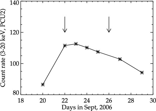
RXTE/PCA light curve of IGR J17497–2821 from September 20–29. Plotted are the mean net counts of PCU2 for each obsID. The time of the two XMM–Newton follow-up observations are marked by arrows.
We processed the XMM–Newton observation data files, using the Science Analysis Software (sas version 14.0), by applying the latest calibration files available as on 2015 January 9. In the imaging mode MOS1 data, the source was affected with severe pile-up and we did not use the MOS1 data further. The EPIC-pn camera and the central CCD of MOS2 camera were operated in the timing mode in both the observations. In this mode only one CCD chip is operated and the data are collapsed into a one-dimension row and read out at high speed, with the second dimension replaced by timing information. This allows a time resolution of 30 μs for EPIC-pn and 1.75 ms for MOS2. From the EPIC-pn/MOS2 timing-mode data we have created images of the source using the sas task ‘EVSELECT’. In the timing mode, the RAWY coordinate gives the timing information and hence the source is visible as a bright strip when plotting RAWX against RAWY.
To check whether the data were affected with soft proton flaring, the light curve was extracted by selecting events with PATTERN = 0 and energy in the range 10–12 keV. No evidence for flaring particle background in the EPIC-pn and MOS2 data was found as the count rates were steady. Due to this reason we did not apply any filtering. The EPIC-pn cleaned event list was extracted by selecting events with PATTERN ≤ 4, FLAG = 0 and energy in the 0.3–10 keV range. From the EPIC-pn cleaned event list, we extracted source events from a 143.5 arcsec (RAWX = 20–55) wide box centred on the source position. For background, we used a rectangular box with RAWX = 3–18. Using the sas task EPATPLOT, we evaluated the pile-up fraction for both the EPIC-pn data sets and found no significant photon pile-up. We used the source and background event lists to create the source and background spectra for both the data sets. We generated the response matrix and ancillary response files using the sas task RMFGEN and ARFGEN, respectively. We followed a similar procedure to extract source and background spectra from the second observation. We rebinned the EPIC-pn spectra to over sample the full width at half-maximum (FWHM) of the energy resolution by a factor of 5 and to have a minimum of 20 counts per bin.
For the MOS2 timing-mode data, we used events with PATTERN = 0, FLAG = 0 and energy in the 0.3–10 keV range. We used rectangular regions of width RAWX = 270–338 (74.8 arcsec) for the source and 260–270 for the background and extracted the source and background spectra. We have also extracted the background spectra from the MOS2 imaging mode data. The generation of the response files and grouping of the source spectra were performed in the same way as done for EPIC-pn data. Although it has been recommended to use the imaging mode background for the MOS2 timing-mode data,1 we formed two sets of MOS2 spectral data with the timing-mode source spectrum in combination with (i) the timing-mode MOS2 background spectrum and (ii) imaging mode MOS2 background spectrum. We grouped both the data sets in the same way as done for the EPIC-pn data, and compared the two MOS2 data sets with different backgrounds. We fitted simple absorbed power-law model to each of the two sets. We found that the two MOS2 background spectra result in largely similar residuals. However, in simultaneous EPIC-pn and MOS2 spectral fitting, we found slightly larger discrepancy if we used the MOS2 spectral data with the imaging mode background. Hence we have used the timing-mode background spectrum for further analysis. There still remains a small discrepancy between the EPIC-pn and MOS2 spectra, which is consistent with calibration uncertainty (Read, Guainazzi & Sembay 2014).
For the analysis of the data of the Reflection Grating Spectra (RGS), we used RGSPROC tool to reduce and extract calibrated source and background spectrum and response files. We extracted the light curve from the data contained in outer CCD (CCD number = 9) to check for particle background. GTI correction was applied with expression rate<=0.2. Spectra and response files of first order obtained from RGS1 and RGS2 were combined by using the sas task RGSCOMBINE. We grouped the spectra with minimum 15 counts per bin by using GRPPHA.
3 SPECTRAL ANALYSIS
We used xspec version 12.8.1g (Arnaud 1996) to perform the spectral analysis. We begin with spectral analysis of the EPIC-pn and MOS2 data obtained from the obs 1. We first fit the 2–10 keV data with a simple power-law model modified by the tbabs (Wilms, Allen & McCray 2000) component to account for the Galactic absorption. Verner cross-section (Verner et al. 1996) and Wilm abundance (Wilms et al. 2000) are applied in tbabs. A model constant is applied to account for relative normalization between the instruments. Power-law index Γ is tied for the pn and MOS2 data. The simple power-law model resulted in Γ ∼ 1.5 and χ2 = 524.3 for 416 degrees of freedom (dof). Extrapolating the power law to low energies revealed a broad excess below 2 keV which is likely the thermal emission from an accretion disc. Performing the fit over the 0.3–10 keV (pn and MOS2), the absorbed power law resulted in χ2/dof = 2801/558. Addition of a multicolour disc blackbody component diskbb (Mitsuda et al. 1984) improved the fit (χ2/dof = 1870/556). The resulting fit showed a broad excess at 1keV in the EPIC-pn data from both the observations. However, the broad excess was not seen in the MOS2 data. To investigate this discrepancy, we attempted to fit the EPIC-pn, MOS2 and RGS data simultaneously. Due to lack of counts, we excluded RGS data below 1 keV.
Fig. 2 shows the observed EPIC-pn, MOS2 and RGS data, folded model and the residuals. The data sets agree well above 1.2 keV. Unfortunately, we cannot verify the 1-keV excess with the RGS data. However, similar excess in the timing-mode data have also been reported by several authors (Boirin et al. 2005; Martocchia et al. 2006; Sala et al. 2008; Hiemstra et al. 2011). We find that the EPIC-pn and MOS2 data show excess emission below ∼1.2 keV but with different shapes. The origin of this excess is not clearly understood and may well be related to instrumental calibration. We thus excluded the 0.3–1.2 keV band data from the subsequent spectral analysis. We have also excluded RGS data due to its poor signal-to-noise ratio.
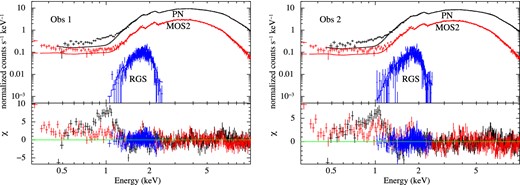
The EPIC-pn, MOS2 and RGS observed data, the model const×tbabs×(diskbb+powerlaw) simultaneously fitted to these data sets. The residuals of obs 1 (left-hand panel) and obs 2 (right-hand panel) show clear discrepancy between the these data sets below ∼1.2 keV.
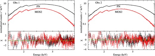
The EPIC-pn and MOS2 observed data and the best-fitting const×tbabs×(diskbb+powerlaw) model (top panel) and residuals (bottom panel) for obs 1 (left) and obs 2 (right). The residuals show possible presence of emission features at ∼6.4 keV.

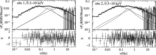
The unfolded EPIC-pn+MOS2 spectral data and the best-fitting model tbabs×(diskbb+nthcomp+diskline) (see Tables 2 and 3 for best-fitting parameters) and deviations of the observed data from the model. Emission line at ∼6.6 keV (obs 1 and 2) can be identified as the broad iron Kα line modelled as diskline.
The absorbed disc blackbody plus power-law model fits the 1.2–10 keV data from obs 1, reasonably well. The reduced χ2 is 1.31 for 476 dof. Examination of the residuals from this fit reveals an excess features like emission lines at ∼3.9 keV and ∼6.4 keV (see Fig. 3). In order to model the structure around ∼6.4 keV, a Gaussian emission feature with an energy of |$6.3_{-0.1}^{+0.1} \,{\rm keV}$| and width (σ) of <0.2 keV was first added to the existing model. This improves the fit with Δχ2 = −37.2 for three parameters. We also fit the data obtained from the obs 2 with the same model, which resulted in χ2/dof = 652.1/472. The feature ∼3.9 keV is very weak and its exact nature is not clear to us. The Gaussian line at ∼6.3 keV has substantial velocity width (∼27 000 km s−1 for obs 1 and obs 2) and can be readily identified with a broadened fluorescent iron Kα emission line from the accretion disc. To account for the relativistic broadening of the line, we replaced the Gaussian component at ∼6.3 keV with the diskline model (Fabian et al. 1989). This resulted in χ2/dof = 590.7/472 for obs 1 (Table 2, model 1) and χ2/dof = 651.2/471 for obs 2. (Table 3, model 1)
List of observations of IGR J17497–2821 by XMM–Newton.
| Obs.ID | Date of | Exposure | Offset | Count ratea |
|---|---|---|---|---|
| observation | time (ks) | (arcmin) | (counts s−1) | |
| 0410580401(obs 1) | 2006 Sep. 22 | 33 | 0.053 | 43.5 |
| 0410580501(obs 2) | 2006 Sep. 26 | 32 | 0.051 | 39.4 |
| Obs.ID | Date of | Exposure | Offset | Count ratea |
|---|---|---|---|---|
| observation | time (ks) | (arcmin) | (counts s−1) | |
| 0410580401(obs 1) | 2006 Sep. 22 | 33 | 0.053 | 43.5 |
| 0410580501(obs 2) | 2006 Sep. 26 | 32 | 0.051 | 39.4 |
aNet count rate is taken from the XMM–Newton EPIC pn timing-mode data after choosing a source region of width 15 pixel from the centre in the 0.3–10 keV energy band and applying standard filtering criteria (see Section 2).
Best-fitting spectral model parameters of IGR J17497–2821 based on the combined spectral analysis of EPIC-pn and MOS2 data sets from obs1.
| obs1 (obs.ID : 0410580401) | |||||
|---|---|---|---|---|---|
| Model component | Parameter | Model 1 | Model 2 | Model 3 | Model 4 |
| constant | 1.0(fixed)(pn) | 1.0(fixed)(pn) | 1.0(fixed)(pn) | 1.0(fixed)(pn) | |
| |${0.9_{-0.004}^{+0.004}}$|(MOS2) | |${0.7_{-0.008}^{+0.007}}$|(MOS2) | |${0.9_{-0.004}^{+0.004}}$|(MOS2) | |${0.9_{-0.004}^{+0.004}}$|(MOS2) | ||
| tbabs | NH(×1022 cm−2) | |${7.5_{-0.1}^{+0.1}}$| | |${7.5_{-0.1}^{+0.1}}$| | |$7.5_{-0.1}^{+0.1}$| | |$7.6_{-0.1}^{+0.1}$| |
| diskbb | kTin(keV) | |$0.2_{-0.006}^{+0.006}$| | |$0.2_{-0.006}^{+0.006}$| | |$0.2_{-0.006}^{+0.006}$| | |$0.2_{-0.006}^{+0.006}$| |
| Norm(×105) | |$2.9_{-0.7}^{+1.0}$| | |$3.1_{-0.8}^{+1.0}$| | |$2.8_{-0.7}^{+1.0}$| | |$3.3_{-0.8}^{+1.1}$| | |
| diskline | Eline (keV) | |$6.5_{-0.3}^{+0.2}$| | |$6.6_{-0.4}^{+0.1}$| | |$6.5_{-0.3}^{+0.2}$| | |$6.6_{-0.4}^{+0.2}$| |
| β | −3.0(fixed) | −3.0(fixed) | −3.0(fixed) | −3.0(fixed) | |
| rin(rg) | |$14.6_{-6.5}^{+952.1}$| | |$11.5_{-3.8}^{+203.6}$| | |$20.3_{-11.4}^{+968.6}$| | |$14.3_{-6.5}^{+235.3}$| | |
| rout(rg) | 1000(fixed) | 1000(fixed) | 1000(fixed) | 1000(fixed) | |
| Inclination (θ) | |$13.8_{\rm peg}^{+25.6}$| | |$15.2_{\rm peg}^{+43.0}$| | |$11.2_{\rm peg}^{+35.2}$| | |$13.4_{\rm peg}^{+41.8}$| | |
| fline(×10−4) | |$1.5_{-0.6}^{+0.7}$| | |$1.9_{-0.8}^{+0.7}$| | |$1.2_{-0.4}^{+0.9}$| | |$1.6_{-0.6}^{+0.8}$| | |
| powerlaw | Γ | |$1.5_{-0.01}^{+0.01}$| | |||
| Norm | |$0.1_{-0.002}^{+0.002}$| | ||||
| simpl | Γ | |$1.5_{-0.02}^{+0.01}$| | |||
| Fracsctr | |$0.03_{-0.005}^{+0.004}$| | ||||
| comptt | T0(keV) | |$0.2_{-0.006}^{+0.006}$|a | |||
| τ | |$0.7_{-0.02}^{+0.02}$| | ||||
| norm(× 10−3) | |$3.8_{-0.05}^{+0.06}$| | ||||
| nthcomp | Γ | |$1.50_{-0.01}^{+0.01}$| | |||
| kTbb(keV) | |$0.2_{-0.006}^{+0.006}$|b | ||||
| Norm | |$0.1_{-0.002}^{+0.002}$| | ||||
| χ2/dof | 590.7/472 | 651.2/472 | 590.0/472 | 592.2/472 | |
Notes. We used const×tbabs×(continuum+diskbb+diskline) to fit spectrum. For continuum component, we applied powerlaw, simpl, comptt and nthcomp in model 1, 2, 3 and 4 respectively.
aand bparameters tied with kTin parameter of diskbb.
Best-fitting spectral model parameters of IGR J17497–2821 based on the combined spectral analysis of EPIC-pn and MOS2 data sets from obs 2.
| obs 2 (obs.ID : 0410580501) | |||||
|---|---|---|---|---|---|
| Model component | Parameter | Model 1 | Model 2 | Model 3 | Model 4 |
| constant | 1.0(fixed)(pn) | 1.0(fixed)(pn) | 1.0(fixed)(pn) | 1.0(fixed)(pn) | |
| |${0.9_{-0.004}^{+0.004}}$|(MOS2) | |${0.7_{-0.008}^{+0.006}}$|(MOS2) | |${0.9_{-0.004}^{+0.004}}$|(MOS2) | |${0.9_{-0.004}^{+0.004}}$|(MOS2) | ||
| tbabs | NH(×1022 cm−2) | |${7.6_{-0.1}^{+0.1}}$| | |${7.5_{-0.1}^{+0.1}}$| | |$7.5_{-0.1}^{+0.1}$| | |$7.7_{-0.1}^{+0.05}$| |
| diskbb | kTin(keV) | |$0.2_{-0.006}^{+0.005}$| | |$0.2_{-0.004}^{+0.004}$| | |$0.2_{-0.006}^{+0.006}$| | |$0.2_{-0.006}^{+0.005}$| |
| Norm(×105) | |$3.5_{-0.8}^{+1.1}$| | |$3.5_{-0.8}^{+1.3}$| | |$3.4_{-0.8}^{+1.1}$| | |$4.0_{-0.9}^{+1.3}$| | |
| diskline | Eline (keV) | |$6.6_{-0.5}^{+0.2}$| | |$6.6_{-0.2}^{+0.1}$| | |$6.6_{-0.5}^{+0.2}$| | |$6.6_{-0.2}^{+0.2}$| |
| β | −3.0(fixed) | −3.0(fixed) | −3.0(fixed) | −3.0(fixed) | |
| rin(rg) | |$11.5_{-3.8}^{+80.1}$| | |$10.8_{-4.1}^{+40.3}$| | |$11.7_{-3.8}^{+90.0}$| | |$11.2_{-3.8}^{+41.8}$| | |
| rout(rg) | 1000(fixed) | 1000(fixed) | 1000(fixed) | 1000(fixed) | |
| Inclination (θ) | |$13.2_{\rm peg}^{+31.7}$| | |$15.1_{\rm peg}^{+12.9}$| | |$13.7_{\rm peg}^{+46.8}$| | |$13.9_{\rm peg}^{+11.5}$| | |
| fline(×10−4) | |$1.5_{-0.5}^{+0.6}$| | |$1.9_{-0.5}^{+0.6}$| | |$1.5_{-0.5}^{+0.6}$| | |$1.6_{-0.5}^{+0.7}$| | |
| powerlaw | Γ | |$1.5_{-0.01}^{+0.01}$| | |||
| Norm | |$0.1_{-0.002}^{+0.002}$| | ||||
| simpl | Γ | |$1.5_{-0.01}^{+0.01}$| | |||
| Fracsctr | |$0.02_{-0.004}^{+0.004}$| | ||||
| comptt | T0(keV) | |$0.2_{-0.006}^{+0.006}$|a | |||
| τ | |$0.8_{-0.02}^{+0.02}$| | ||||
| Norm(× 10−3) | |$3.5_{-0.05}^{+0.05}$| | ||||
| nthcomp | Γ | |$1.5_{-0.01}^{+0.01}$| | |||
| kTbb(keV) | |$0.2_{-0.006}^{+0.005}$|b | ||||
| Norm | |$0.1_{-0.001}^{+0.002}$| | ||||
| χ2/dof | 651.2/471 | 741.7/471 | 651.3/471 | 651.5/471 | |
Notes. We used const×tbabs×(continuum+diskbb+diskline) to fit spectrum. For continuum component, we applied powerlaw, simpl, comptt and nthcomp in model 1, 2, 3 and 4 respectively.
aand bparameters tied with kTin parameter of diskbb.
To describe the continuum with a more physical model, we have also fitted the continuum with the nthcomp model (Zdziarski, Johnson & Magdziarz 1996; Życki, Done & Smith 1999). Fitting the 1.2–10 keV data from obs 1 with the tbabs×(diskbb+nthcomp) model provided an acceptable fit with χ2/dof = 630.8/476. Here the fitting residuals also showed the same emission features around the same energy. In order to investigate the relativistic broadening of the line, we replaced the Gaussian line with the diskline model (see Fig. 4). This resulted in χ2/dof = 592.2/472 for obs 1 (Table 2, model 4) and χ2/dof = 651.5/471 for obs 2 (Table 3, model 4). We fixed the emissivity index (β) and the outer radius of the disc to the value −3.0 and 1000rg respectively for both the observations. The best-fitting parameter values for different models are reported in Tables 2 and 3 for obs 1 and 2, respectively.
We have also checked for the variation of iron line energy and disc blackbody parameters by using different continuum models such as powerlaw, simpl (Steiner et al. 2009), comptt (Hua & Titarchuk 1995; Titarchuk & Lyubarskij 1995) and nthcomp. We find that the best-fitting parameters of the iron line and the thermal accretion disc are consistent within error for the different continuum models (Tables 2 and 3).
4 TEMPORAL ANALYSIS
4.1 The timing-mode XMM–Newton EPIC-pn data
The timing-mode EPIC-pn data with a time resolution of 30 μs are well suited to study temporal behaviour of IGR J17497–2821. We used the General High-energy Aperiodic Timing Software (ghats) software package (version 1.1.0)2 for our timing analysis. We first generate the PDSs over the entire 0.3–10 keV band from the source event lists for both the observations. The data were divided into time segments of length 786 s, and a Fourier transform was performed with the Nyquist frequency set at ∼42 Hz. The resulting PDSs were Poisson noise corrected (van der Klis 1995a) and logarithmically rebinned. The PDSs were evaluated using rms normalization (Belloni & Hasinger 1990; van der Klis 1995b).
The XMM–Newton PDSs of obs 1 and obs 2 of IGR J17497–2821 derived from the full band EPIC-pn fitted with three Lorentzians (top panel) and residuals (bottom panel). The PDSs were derived from the high time resolution (30 μs) EPIC-pn data obtained from obs 1 and obs 2 with XMM–Newton.
Results of fits to the PDSs of IGR J17497–2821 derived from the timing-mode EPIC-pn data. Frequency range 0.01–40 Hz has been used to calculate the integrated rms.
| Model componenta | Parameter b | 0.3–2 keV | 2–5 keV | 5–10 keV | 0.3–10 keV |
|---|---|---|---|---|---|
| obs 1 (obs.ID : 0410580401) | |||||
| LFN | 2Δ (Hz) | |$0.1_{-0.02}^{+0.03}$| | 0.1 ± 0.01 | |$0.1_{-0.01}^{+0.01}$| | 0.1 ± 0.01 |
| Norm | |$6.07^{+0.9}_{-0.9} \times 10^{-02}$| | |$5.8^{+0.4}_{-0.5} \times 10^{-02}$| | |$6.4^{+0.3}_{-0.4} \times 10^{-02}$| | |$6.1^{+0.3}_{-0.4} \times 10^{-02}$| | |
| HFN | 2Δ (Hz) | |$4.1_{-1.4}^{+2.0}$| | |$2.5_{-0.9}^{+1.7}$| | |$3.0_{-0.8}^{+1.0}$| | |$3.3_{-0.6}^{+0.7}$| |
| Norm | |$0.1^{+0.03}_{-0.03}$| | |$2.9^{+0.9}_{-1.0} \times 10^{-02}$| | |$3.7^{+0.5}_{-0.6} \times 10^{-02}$| | |$3.1^{+0.3}_{-0.4} \times 10^{-02}$| | |
| MFN | ν0 (Hz) | – | |$0.3_{-0.08}^{+0.05}$| | |$0.3_{-0.05}^{+0.04}$| | |$0.3_{-0.05}^{+0.04}$| |
| 2Δ (Hz) | – | |$0.4_{-0.2}^{+0.2}$| | |$0.3_{-0.1}^{+0.2}$| | |$0.4_{-0.1}^{+0.1}$| | |
| Norm | – | |$1.8^{+1.3}_{-1.0} \times 10^{-02}$| | |$1.4^{+0.7}_{-0.5} \times 10^{-02}$| | |$2.0^{+0.7}_{-0.5} \times 10^{-02}$| | |
| Significance (σ)c | – | 2.8 | 3.9 | 5.9 | |
| Integrated rms (in percentage) | |$43.0^{+1.0}_{-1.0}$| | |$32.0^{+0.3}_{-0.3}$| | |$33.0^{+0.4}_{-0.4}$| | |$32.3^{+0.2}_{-0.2}$| | |
| mean count rate(counts s−1)d | 2.8 | 23.3 | 17.8 | 43.8 | |
| χ2/dof | 88.0/104 | 140.9/133 | 200.1/192 | 152.0/163 | |
| obs 2 (obs.ID : 0410580501) | |||||
| LFN | 2Δ (Hz) | |$0.1_{-0.02}^{+0.03}$| | 0.1 ± 0.01 | |$0.1_{-0.01}^{+0.01}$| | 0.1 ± 0.01 |
| Norm | |$6.3^{+1.0}_{-1.0} \times 10^{-02}$| | |$6.0^{+0.3}_{-0.3} \times 10^{-02}$| | |$6.5^{+0.4}_{-0.4} \times 10^{-02}$| | |$6.3^{+0.3}_{-0.3} \times 10^{-02}$| | |
| HFN | 2Δ (Hz) | |$3.2_{-1.2}^{+2.1}$| | |$1.9_{-0.4}^{+0.6}$| | |$3.9_{-1.2}^{+1.8}$| | |$2.4_{-0.4}^{+0.5}$| |
| Norm | |$0.1^{+0.04}_{-0.03}$| | |$4.1^{+0.5}_{-0.7} \times 10^{-02}$| | |$3.3^{+0.5}_{-0.6} \times 10^{-02}$| | |$3.6^{+0.4}_{-0.4} \times 10^{-02}$| | |
| MFN | ν0 (Hz) | – | |$0.3_{-0.04}^{+0.03}$| | |$0.3_{-0.04}^{+0.03}$| | |$0.3_{-0.04}^{+0.03}$| |
| 2Δ (Hz) | – | |$0.2_{-0.1}^{+0.2}$| | |$0.4_{-0.1}^{+0.1}$| | |$0.3_{-0.09}^{+0.1}$| | |
| Norm | – | |$9.3^{+8.0}_{-4.9} \times 10^{-03}$| | |$2.0^{+0.8}_{-0.6} \times 10^{-02}$| | |$1.5^{+0.6}_{-0.5} \times 10^{-02}$| | |
| Significance (σ)c | – | 2.9 | 5.0 | 5.0 | |
| Integrated rms (in percentage) | |$44.0^{+1.8}_{-1.5}$| | |$33.0^{+0.3}_{-0.2}$| | |$34.0^{+0.5}_{-0.4}$| | |$32.6^{+0.2}_{-0.2}$| | |
| mean count rate(counts s−1)d | 2.6 | 21.2 | 16.2 | 39.9 | |
| χ2/dof | 90.9/104 | 130.8/133 | 207.1/192 | 181.2/192 | |
aLFN and HFN are Lorentzian components used to model the low- and high-frequency noise. The centroid frequencies of the LFN and HFN components were frozen to zero. MFN is the mid-frequency Lorentzian used to fit broad feature between low- and high-frequency noise components in the PDS. Sum of two Lorentzians are applied for energy band 0.3–2 keV, whereas sum of three Lorentzians are applied for energy bands 2–5, 5–10 and 0.3–10 keV.
bν0 and 2Δ are the centroid frequency and FWHM of the Lorentzian, respectively.
cThe significance of the middle component computed with 1 σ error is presented separately.
dmean count rate is calculated from light curves in the 0.3–2, 2–5, 5–10 and 0.3–10 keV band after applying standard filtering and taking source region of 15 pixel width.
Results of fits to the PDS of RXTE/PCA observations on 2006 September 20 and 23. Frequency range 0.01–64 Hz is used to calculate the rms.
| obsID | Model component | Parameter | 2–5 keV | 5–10 keV | 10–20 keV |
|---|---|---|---|---|---|
| LFN | 2Δ (Hz) | |$0.1_{-0.02}^{+0.02}$| | |$0.1_{-0.02}^{+0.02}$| | |$0.1_{-0.02}^{+0.02}$| | |
| Norm | |$2.6^{+0.4}_{-0.4} \times 10^{-02}$| | |$2.7^{+0.2}_{-0.3}\times 10^{-2}$| | |$4.2^{+0.4}_{-0.4}\times 10^{-2}$| | ||
| 92016-01-01-00 | HFN | 2Δ (Hz) | |$1.0_{-0.2}^{+0.3}$| | |$2.9_{-0.7}^{+1.1}$| | |$3.7_{-0.9}^{+1.2}$| |
| (20 Sep. 2006) | Norm | 2.3 ± 0.3 × 10⁻² | |$1.5^{+0.3}_{-0.3}\times 10^{-2}$| | |$2.0^{+0.3}_{-0.3}\times 10^{-2}$| | |
| MFN | ν0 (Hz) | |$0.3_{-0.08}^{+0.05}$| | |$0.3_{-0.05}^{+0.04}$| | ||
| 2Δ (Hz) | |$0.4_{-0.1}^{+0.2}$| | |$0.3_{-0.09}^{+0.1}$| | |||
| Norm | |$1.0^{+0.6}_{-0.4}\times 10^{-2}$| | |$1.4^{+0.5}_{-0.4}\times 10^{-2}$| | |||
| Significance (σ)a | 4.0 | 5.4 | |||
| Integrated rms (in percentage) | |$21.3^{+0.2}_{-0.3}$| | |$22.3^{+0.2}_{-0.3}$| | |$26.7^{+0.3}_{-0.3}$| | ||
| χ2/dof | 141.8/136 | 159.6/156 | 220.1/201 | ||
| LFN | 2Δ (Hz) | |$7.5^{+2.7}_{-2.0} \times 10^{-2}$| | |$7.8^{+2.8}_{-2.1} \times 10^{-2}$| | |$8.3^{+2.8}_{-2.1} \times 10^{-2}$| | |
| Norm | 2.0 ± 0.5 × 10⁻² | 2.3 ± 0.5 × 10⁻² | |$3.3^{+0.7}_{-0.7}\times 10^{-2}$| | ||
| 92016-01-01-02 | HFN | 2Δ (Hz) | |$0.9_{-0.2}^{+0.3}$| | |$0.9_{-0.2}^{+0.2}$| | |$1.0_{-0.2}^{+0.3}$| |
| (23 Sep. 2006) | Norm | |$2.9^{+0.5}_{-0.6} \times 10^{-2}$| | |$3.5^{+0.4}_{-0.4}\times 10^{-2}$| | |$4.4^{+0.6}_{-0.6}\times 10^{-2}$| | |
| Integrated rms (in percentage) | |$21.1^{+0.7}_{-0.7}$| | |$23.1^{+0.4}_{-0.4}$| | |$26.6^{+0.6}_{-0.7}$| | ||
| χ2/dof | 129.0/112 | 114.6/112 | 208.7/204 |
aThe significance of the middle component computed with 1σ error is presented separately.
Results of fits to the 0.01–64 Hz PDS of RXTE/PCA observations on September 24 and 25.
| obsID | Model component | Parameter | 2–5 keV | 5–10 keV | 10–20 keV |
|---|---|---|---|---|---|
| LFN | 2Δ (Hz) | |$0.1_{-0.04}^{+0.05}$| | |$0.1_{-0.04}^{+0.05}$| | |$0.1_{-0.05}^{+0.09}$| | |
| Norm | |$2.8^{+0.7}_{-0.7} \times 10^{-2}$| | |$2.6^{+0.7}_{-0.7}\times 10^{-2}$| | |$4.0^{+1.2}_{-1.2}\times 10^{-2}$| | ||
| 92016-01-02-01 | HFN | 2Δ (Hz) | |$1.4_{-0.6}^{+1.4}$| | |$0.9_{-0.2}^{+0.4}$| | |$1.6_{-0.6}^{+2.0}$| |
| (24 Sep. 2006) | Norm | |$2.5^{+0.7}_{-0.8} \times 10^{-2}$| | |$3.5^{+0.6}_{-0.7}\times 10^{-2}$| | |$4.3^{+0.9}_{-1.0}\times 10^{-2}$| | |
| Integrated rms (in percentage) | |$22.3^{+1.0}_{-1.0}$| | |$23.9^{+0.7}_{-0.7}$| | |$28.0^{+1.0}_{-0.9}$| | ||
| χ2/dof | 155.5/136 | 105.8/112 | 130.5/136 | ||
| LFN | 2Δ (Hz) | |$0.1_{-0.03}^{+0.04}$| | |$0.1_{-0.03}^{+0.03}$| | |$0.1_{-0.03}^{+0.04}$| | |
| Norm | |$2.3^{+0.6}_{-0.6} \times 10^{-2}$| | |$3.0^{+0.6}_{-0.6}\times 10^{-2}$| | |$3.6^{+0.8}_{-0.8}\times 10^{-2}$| | ||
| 92016-01-02-02 | HFN | 2Δ (Hz) | |$0.8_{-0.2}^{+0.3}$| | |$1.0_{-0.2}^{+0.3}$| | |$0.9_{-0.2}^{+0.3}$| |
| (25 Sep. 2006) | Norm | |$2.7^{+0.5}_{-0.5} \times 10^{-2}$| | |$2.8^{+0.5}_{-0.5}\times 10^{-2}$| | |$3.7^{+0.7}_{-0.7}\times 10^{-2}$| | |
| Integrated rms (in percentage) | |$21.5^{+0.4}_{-0.7}$| | |$23.3^{+0.4}_{-0.4}$| | |$26.3^{+0.5}_{-0.5}$| | ||
| χ2/dof | 107.0/112 | 157.3/136 | 180.4/159 |
The shape and nature of the power spectra and rms variability are often found to vary with energy (Belloni et al. 1997; Lin et al. 2000). Such trends gives important clues to the nature of the intrinsic emission processes and cause of the observed variability. Hence, we have divided 0.3–10 keV band EPIC-pn data into three different energy bands 0.3–2, 2–5 and 5–10 keV, for the timing analysis. The main motivation of performing the energy-dependent timing analysis was to identify if the timing characteristics are correlated with the spectral parameters. The choice of the energy bands are indeed empirical to some extent. The low-energy band (0.3–2 keV) was selected to sample the photons which might predominantly originate from the accretion disc. The highest count rate was found to be in the 2–5 keV band, whereas the 0.3–2 keV band had the lowest count rate (see Table 4). Signal-to-noise ratio of the 2–5 keV band data was found to be approximately three times more than that of 0.3–2 keV band for both observations.
We have computed the PDSs of three the energy bands (0.3–2, 2–5 and 5–10 keV) following the method as described earlier. We consider only those components which are detected with 3σ significance or above.3 We find that the MFN component is detected significantly only at high-energy bands (2–5 keV and 5–10 keV).
For obs 1, the 0.3–2 keV band PDS fit well with only the LFN and HFN components (|$\chi ^2 /{\rm {\rm dof}} \sim 88/104$|). The PDS of the 2–5 keV energy band was first fitted with two zero-centred Lorentzian (LFN and HFN) as before, with χ2/dof = 158.31/136. Introducing of a middle component at ∼0.3 Hz improves the fit (χ2/dof = 140.95/133), with the significance of the resulting MFN being ∼3σ. The PDS of the 5–10 keV band similarly required all three Lorentzian components for a satisfactory fit (as shown in Fig. 6).
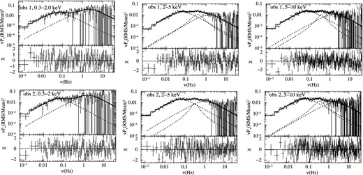
The PDSs of IGR J17497–2821 in different energy bands fitted with Lorentzian (top panel of plots) and residual (bottom panel of plots). The PDSs were derived from the high time resolution (30 μs) EPIC-pn data obtained from obs 1 and obs 2 with XMM–Newton. Sum of two Lorentzians are applied to the PDSs in the 0.3–2 keV band and sum of 3 Lorentzians are applied for the PDSs in the 2–5 and 5–10 keV bands.
To test the possible presence of an MFN component in the 0.3–2 keV band, we applied a Lorentzian with centroid and width fixed to that of the MFN component of the 2–5 keV band. We varied the norm of the applied Lorentzian to obtain a fit to the PDS. The resulting improvement in χ2 was marginal with Δχ2 = −3 for one additional parameter. with the component being 1.5σ significant. Computing the errors with 90 per cent confidence limit, we find the strength of the norm to be |${\sim } 0.014^{+0.014}_{-0.014}$|. Thus, the lower limit is consistent with zero confirming that the component may not be significant. However, the upper limit is comparable to the strength of the MFN in the 2–5 keV band (see Table 4). Quality of the 0.3–2 keV data is poor as compared to the data in the 2–5 keV. This also affects the significance of MFN in low-energy band 0.3–2 keV. This indicates that although the MFN component may not be significant, but we cannot rule out its presence given the current SNR of the data.
The PDSs of obs 2 were fitted in a similar fashion as described above (see Table 4). For both observations, integrated rms values (frequency range 0.01–40 Hz) for PDSs of energy bands 0.3–2, 2–5, 5–10 and 0.3–10 keV are reported in Table 4.
4.2 RXTE/PCA data
To test the energy dependence of the PDS over the course of the outburst we have analysed the available RXTE data in different energy channels. RXTE monitored this source from 2006 September 20 to 29. For south Atlantic anomaly correction, we removed 30 min of data. In this duration, the satellite was exposed to strong radiation. Number of Proportional Counter Units (PCUs) which observe the source is different for different observations. 92016-01-01-00, 92016-01-01-02, 92016-01-02-01 and 92016-01-02-02 have observed the source with 4, 1, 1 and 2 PCU, respectively. In this work, we have performed the timing analysis for all the four observations with GOODXENON event files. The RXTE/PCA timing analysis was performed for the energy bands 2–5, 5–10 and 10–20 keV, respectively with ghats V 1.1.0. The PDSs were created for time segments of length 128 s with a Nyquist frequency of 64 Hz and deadtime corrections were applied (Zhang et al. 1995). Logarithmic rebinning was applied to the Poisson noise corrected PDS. The resulting PDSs were fitted with Lorentzian components as described in Section 4.1. We present in Fig. 7 the PDSs of different energy bands of the RXTE observations and describe the results below.
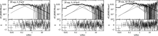
PDSs of RXTE obsID 92016-01-01-00 (September 20) in energy bands 2–5 keV, 5–10 keV and 10–20 keV fitted with Lorentzians (top panel of plots) and residual (bottom panel of plots).
We found that a significant MFN component was detected only in the 5–10 kev and 10–20 keV of obsID 92016-01-01-00 (September 20). The 2–5 keV band was first fitted with the LFN and HFN components (χ2/dof = 141.77/136). The remaining residual structures at ∼0.3 Hz was then fitted with the MFN component to get the final χ2/dof to be 128.86/133. The middle broad noise component was found to be only ∼2.67σ significant, and hence discarded from the final results as we retain only those components with a detection significance above ∼3σ. Signal-to-noise ratio of the data in the 2–5 keV is found to be 1.3 times smaller than the 5–10 keV band. So the presence of MFN cannot be discarded as lower significance of MFN may be due to bad quality data of 2–5 keV band. The PDSs of the 5–10 and 10–20 keV energy ranges were fit in a similar fashion with three Lorentzian components. In both cases the middle component was required for the fit with a significance of ∼4.0σ and ∼5.4σ, respectively (see Tables 5 and 6). Thus similar to the results of XMM–Newton data, a statistically significant MFN component was detected only at the higher energy bands. The PDS of other obsIDs analysed fit well with only two Lorentzian components, with the MFN being not statistically significant.
5 DISCUSSION
In this work, we have presented the spectral and timing analysis of the two XMM–Newton observations on 2006 September 22 (obs 1) and 26 (obs 2) of the black hole X-ray binary IGR J17497–2821. Following the detection of the source as an X-ray nova on 2006 September 17, several X-ray telescopes (RXTE, Swift, INTEGRAL, Suzaku and Chandra) have followed the outburst. The two XMM–Newton observations were performed during the middle of the outburst of IGR J17497–2821 (see Fig. 1).
From our spectral analysis (Section 3), we find that the 1.2–10 keV spectra of IGR J17497–2821 from both the observations are well described by a multicoloured disc blackbody with an inner disc temperature kTin ∼ 0.2 keV and nthcomp continuum model. The absorbed flux is fX = 4.9 × 10⁻¹⁰ erg s−1 cm−2 (EPIC-pn) in the 1.2–10 keV and corresponding absorption corrected fluxes are fX = 8.6 × 10⁻¹⁰ erg s−1 cm−2 (EPIC-pn), for obs 1 (model 4 in Table 2). The distance to the source is not known. Considering its close angular proximity to the Galactic Centre, we assume a distance of ∼8 kpc. This gives the observed luminosity as ∼3.5 × 1036 erg s−1 and absorption corrected luminosity as ∼6.2 × 1036 erg s−1 (EPIC-pn) in the 1.2–10 keV band for obs 1 (model 4 in Table 2). IGR J17497–2821 was slightly fainter in the second observation with an absorbed flux fX = 4.5 × 10⁻¹⁰ erg cm−2 s−1 and corresponding unabsorbed flux fX = 8.3 × 10⁻¹⁰ erg cm−2 s−1 in the 1.2–10 keV band. From the combined analysis of the EPIC-pn and MOS2 data, we find the flux of the disc blackbody component to be ∼5 times lower than that of the power-law component in the 1.2–10 keV range. The strong and hard (Γ ∼ 1.50) (EPIC-pn) power law and a weak disc component are typical of black hole X-ray binaries in the hard state (see e.g. Belloni et al. 2002a; Fender, Belloni & Gallo 2004; Remillard & McClintock 2006).
The results from the XMM–Newton spectral analysis are in keeping with the general trends of the different physical parameters as observed by various X-ray instruments. In Fig. 8, we present the comparison of our results with previous works by Walter et al. (2007, hereafter RW07) on joint spectral fit of Swift/XRT and INTEGRAL data, analysis of Suzaku data by Paizis et al. (2009, hereafter AP09), JR07 for RXTE results and Paizis et al. (2007, hereafter AP07) for analysis of Chandra data. It is difficult to directly compare the different spectral parameters from previous works on this source owing to the different spectral models used for the analysis. However, qualitative trends in the variation of different parameters can be ascertained. The neutral absorption derived from our results (NH ∼ 7.5 × 1022 cm−2) is different from other observations.
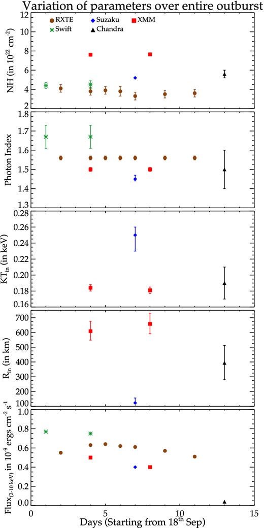
From top to bottom: NH, photon index, kTin, Rin and flux2 − 10 keV, respectively, from spectral fits of data of different X-ray telescopes (marked in different colours). The parameter values plotted have been taken from following references: 1 – Rodriguez et al. (2007) for RXTE (brown), absorbed power law is used to calculate Γ and model phabs×edge×comptt is used to calculate NH and flux; 2 – Walter et al. (2007) for INTEGRAL and Swift (green), absorbed cut-off power law has been used to calculate parameters; 3 - our work for XMM–Newton (red), const×tbabs×(nthcomp+diskbb+diskline) is used to calculate parameters; 4 – Paizis et al. (2009) for Suzaku (blue), model wabs×edge×cutoffpl is used to calculate Γ and wabs×(gauss+diskbb+compps) is used to calculate KTin, NH, Rin and Flux; and 5 – Paizis et al. (2007) for Chandra telescope, phabs×(diskbb+powerlaw+gauss) is used to calculate the parameters. The flux values in the lower panel are the scaled fluxes in the 2–10 keV range derived from broad-band model fits to respective data sets.
The photon index (Γ ∼ 1.50) from the analysis of both observations is consistent with previous estimates from Suzaku data by AP09. However, the Γ inferred from the RXTE and Swift–INTEGRAL observations by JR07 and RW07 during the outburst is significantly different. AP09 ascribe the difference to effects from instrumental cross-calibration. Also, the source being close to the Galactic Centre, possible contamination from the Galactic background may affect spectral analysis of data from RXTE/PCA with wide field of view. Indeed the neutron star Swift J1749.4–2807 (within ∼13 arcmin radius of IGR J17497–2821) was also active during this period as reported by Wijnands et al. (2009). However, the qualitative trend for the results from different instruments is similar, and the Γ was nearly constant during the outburst.
Suzaku and Chandra observations showed the evidence of an accretion disc with inner disc temperature kTin ∼ 0.25 keV and kTin ∼ 0.2 keV, respectively, as reported in AP09 and AP07, respectively. This is consistent with the value obtained for our analysis of the two XMM–Newton observations (kTin ∼ 0.2 keV). To compare with previous results, we have computed the apparent inner disc radius assuming an inclination angle of 60° and distance 8 kpc. We found |$R_{\rm in} = 649_{-84}^{+100}\,{\rm km}$| and |$715_{-85}^{+108}\,{\rm km}$| for obs 1 and obs 2, respectively. Comparing the results we find that the radii estimated from the XMM–Newton and Chandra observations are close in value, within errors, whereas that from the Suzaku data on September 25 is lower than the above estimates, indicating the formation of an accretion disc. However, the discrepancy could also be due to different models and energy bands used for calculation of disc radius with different instruments. The RXTE/PCA light curve (Fig. 1) shows a monotonic variation in the count rate. Fig. 8 shows that the 2–10 keV flux measured with Suzaku is significantly lower by ∼50 per cent than that measured with RXTE/PCA on the same day. This difference is likely to be due to the uncertainties in the absolute flux calibration of RXTE/PCA and the burst and window modes of Suzaku/XISs. The lower inner radius measured with the Suzaku data may be due to the lower diskbb normalization which in turn may be related to the uncertainty in the absolute flux calibration.
The lowest panel of Fig. 8 shows the variation of the flux scaled to the 2–10 keV energy band, calculated from the reported best-fitting model parameters by RW07, JR07, AP07 and AP09. Flux of the source shows gradual decrease with time with the flux on 2006 October 01 (AP07) being nearly 20 times lower than that at the beginning on 2006 September 19. We have presented the variation of hardness ratio (ratio of counts in 8.6–18 keV to 5.0–8.6 keV energy bands) as defined in Remillard & McClintock 2006) with the average PCU2 counts (5–18 keV) in Fig. 9. The source is clearly seen to have hardness ≥0.76 throughout the outburst. From the overall results of the spectral analysis, the source appears to stay in the hard state during its entire outburst with Γ ≤ 2.
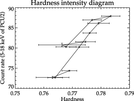
Hardness intensity diagram with X-axis representing the hardness of the source and Y-axis the PCU2 counts for 5–18 keV energy range. The hardness is defined as the ratio of the counts in the energy band 8.6–18 keV to 5.0–8.6 keV, following Remillard & McClintock (2006).
Although differing in frequency and energy range, the full band (0.3–10 keV) PDS derived from the timing-mode EPIC-pn data are similar to that obtained from the RXTE data performed by JR07. As in JR07, we require three Lorentzian components to fit the PDS (LFN, MFN and HFN for ν ≥ 1 Hz). Such broad features is typical of black hole binaries (e.g. Cyg x-1 and GX 339–4; Nowak 2000). Characteristic frequencies of LFN, HFN and MFN are consistent with the JR07. For same frequency (0.01–40 Hz) and energy (2–10 keV) range, the fit parameters of the LFN, MFN and HFN are similar for both the RXTE and XMM–Newton observations. However, the integrated rms for the XMM–Newton data were found to be ∼32 per cent, larger than that of the RXTE (∼23 per cent).
Based on our energy-dependent timing analysis of XMM–Newton and RXTE, we find that the timing behaviour of IGR J17497–2821 strongly depends on the energy band. The MFN feature is not present in the low-energy band [0.3–2 keV (XMM–Newton), 2–5 keV (RXTE)], which could be due to poor signal-to-noise ratio in this band. But variation of rms is found to be strongly dependent on energy bands. Softer energy bands had higher fractional rms e.g. rms of the energy band 0.3–2 keV of XMM–Newton data was nearly ∼1.3 times that of the energy bands 2–5 and 5–10 keV. However, at higher energies, the rms variability was found to increase with energy. Such a behaviour though typical for black holes in high/soft state (Belloni et al. 1997), is not common for sources in hard state. Increased variability at higher energy in the hard state of some sources e.g. 1E 1740.7-2942 and Cyg X-1 have been reported by Lin et al. (2000).
Also, we see from Fig. 10, that the magnitude of the rms variability is lower for RXTE observations than that of XMM data. A possible reason for the above could be increase of the mean flux due to contribution from the galactic ridge emission to the RXTE data (see Section 5). Although the accreting millisecond pulsar Swift J1749.4–2807, within the RXTE field of view of IGR J17497–2821, was also present in outburst at the same time (Wijnands et al. 2009), its flux was ∼3000 times less than that of IGR J17497–2821, could not have contributed to the background.
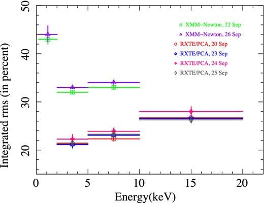
Variation of integrated rms with different energy bands for XMM–Newton/EPIC-pn and RXTE/PCA observations. Frequency range 0.01–40 Hz is used to calculate rms. The rms values are of 68 per cent confidence limit.
The authors would like to extend sincere thanks to the referee for his/her critical comments which has contributed considerably in improving the work. The authors would also like to thank the organizing committee of the 2nd X-ray Astronomy School at IUCAA during 2013 February 4 to March 2, where this work was initiated. MSA and ASM would also like to thank IUCAA for hosting them during subsequent visits. SJ and GCD acknowledge support from grant under ISRO-RESPOND programme (ISRO/RES/2/384/2014-15). MSA would like to acknowledge fellowship provided under ISRO-RESPOND programme. BR likes to thank IUCAA for the hospitality and facilities extended to him under their Visiting Associateship programme. This research has made use of the ghats package developed by Dr Tomaso Belloni at INAF – Osservatorio Astronomico di Brera. The authors also like to thank Dr Dipankar Bhattacharya, Dr Ranjeev Misra and Dr Tomaso Belloni for helpful suggestions and discussions.
http://xmm2.esac.esa.int/docs/documents/CAL-TN-0018.pdf (see XMM-SOC-CAL-TN-18, 2014 September 1), we have compared the MOS2 spectra by using both imaging mode background from the outer CCDs and timing-mode background from the central CCD.
Obtained by dividing the norm of the component with the lower limit of the error computed with 1σ confidence interval.
Observed at the end of the 1998 outburst of XTE J1748-288.
REFERENCES
APPENDIX A: DIMINISHED RMS VARIABILITY DUE TO CONTAMINATION FROM THE GALACTIC RIDGE EMISSION
RXTE/PCA being a non-imaging detector with a large field of view, is more susceptible to contamination from background X-ray flux due to the Galactic ridge emission, as opposed to XMM–Newton. Excess background can lower the net observed fractional rms variability (rms/mean). Following Rodriguez et al. (2007) if we consider the RXTE obsID 30185-01-20-004 to represent the Galactic background emission, the mean count rate of the background emission then was found to be ∼30 counts s−1 in the 2–10 keV band. Using the webpimms tool,5 we find the equivalent RXTE/PCA count rate of the 2–10 keV flux of IGR J17497–2821 measured with XMM–Newton to be 51 counts s−1. Thus the sum of the estimated RXTE/PCA count rate and the Galactic background is ∼81 counts s−1. This is similar to the mean 2–10 keV count rate of 80 counts s−1 measured from the RXTE obsID 92016-01-00. Thus it is entirely possible that the addition of background flux due to the Galactic ridge emission to the source flux can lower the observed rms variability of IGR J17497–2821, as seen in our case.
