


Abstract
We have mapped the superwind/halo region of the nearby starburst galaxy M82 in the mid-infrared with Spitzer − IRS. The spectral regions covered include the H2 S(1)–S(3), [Ne ii], [Ne iii] emission lines and polycyclic aromatic hydrocarbon (PAH) features. We estimate the total warm H2 mass and the kinetic energy of the outflowing warm molecular gas to be between Mwarm ∼ 5 and 17 × 106 M⊙ and EK ∼ 6 and 20 × 1053 erg. Using the ratios of the 6.2, 7.7 and 11.3 μm PAH features in the IRS spectra, we are able to estimate the average size and ionization state of the small grains in the superwind. There are large variations in the PAH flux ratios throughout the outflow. The 11.3/7.7 and the 6.2/7.7 PAH ratios both vary by more than a factor of 5 across the wind region. The northern part of the wind has a significant population of PAH's with smaller 6.2/7.7 ratios than either the starburst disc or the southern wind, indicating that on average, PAH emitters are larger and more ionized. The warm molecular gas to PAH flux ratios (H2/PAH) are enhanced in the outflow by factors of 10–100 as compared to the starburst disc. This enhancement in the H2/PAH ratio does not seem to follow the ionization of the atomic gas (as measured with the [Ne iii]/[Ne ii] line flux ratio) in the outflow. This suggests that much of the warm H2 in the outflow is excited by shocks. The observed H2 line intensities can be reproduced with low-velocity shocks (v < 40 km s−1) driven into moderately dense molecular gas (102 < nH < 104 cm−3) entrained in the outflow.
1 INTRODUCTION
Galactic outflows, ‘superwinds’, are driven by hot gas and momentum generated by the combined mechanical and radiative energy and momentum output from stellar winds and supernovae (e.g. Heckman, Armus & Miley 1990). They have been invoked as a source for the heating and metal-enrichment of both the intracluster and intergalactic medium (Adelberger et al. 2003; Loewenstein 2004), as a major driver of galaxy evolution (e.g. Croton et al. 2006), and as playing a crucial role in establishing the mass–metallicity relation among galaxies (Tremonti et al. 2004). Superwinds have also been hypothesized to be the mechanism through which a dust enshrouded ultraluminous infrared galaxy (ULIRG) transitions to an optically identified quasar (e.g. Sanders et al. 1988).
The dynamical evolution of a starburst-driven outflow has been extensively discussed (e.g. Chevalier & Clegg 1985; Suchkov et al. 1994; Wang 1995; Tenorio-Tagle & Muñoz-Tuñon 1998; Strickland & Stevens 2000). Superwinds are generated when the kinetic energy in the outflow from massive stars and supernovae is thermalized, generating a region of very hot (T ∼ 108 K) low-density gas in the (interstellar medium) ISM of a starburst galaxy (Chevalier & Clegg 1985). This hot gas will expand, sweeping-up and entraining ambient gas and creating a hot cavity within the overall structure of the ISM. This region of hot gas is highly overpressurized relative to its surrounding ambient ISM and will expand along the steepest pressure gradients. As it expands, it sweeps up and shocks ambient material, creating an outflowing ‘superwind’ (Castor, McCray & Weaver 1975; Weaver et al. 1977). Contributing to this overall energy driven outflow is the radiation pressure on dust grains that are likely coupled to the ionized gas within the flow (Murray, Quataert & Thompson 2005).
There is a significant amount of morphological, physical and kinematic evidence for the existence of superwinds in nearby starburst and infrared luminous galaxies (e.g. Heckman et al. 1990). Large- scale optical emission-line and associated X-ray nebulae are ubiquitous in starbursts (Heckman et al. 1990; Lehnert, Heckman & Weaver 1999; Strickland et al. 2004), and these increase in size and luminosity from dwarf starbursts to ULIRGs, where they can be tens of kpc in size (Grimes et al. 2005). In addition, the winds are observed in molecular lines such as CO (Walter, Weiss & Scoville 2002; Bolatto et al. 2013) and blueshifted absorption features (e.g. Na D) seen projected against the starburst nuclei (Heckman et al. 2000; Martin 2005; Rupke & Veilleux 2005) indicating that the neutral, cold ISM is being swept-up in the outflow. Recently, vigorous outflows have also been detected in ULIRGs and LIRGs in molecular absorption lines with Herschel-PACS which suggest very high mass outflow rates (e.g. Fischer et al. 2010; Sturm et al. 2011; Spoon et al. 2013; Veilleux et al. 2013). ULIRGs which have higher AGN bolometric fractions appear to have higher terminal velocities and shorter gas depletion time-scales than those with lower AGN bolometric fractions, suggesting that at least in ULIRGs, the AGN power is related to the feedback on the cold molecular gas (Veilleux et al. 2013; Cicone et al. 2014).
M82 is the brightest, nearest, and best-studied starburst galaxy with an outflow (Heckman et al. 1990; Shopbell & Bland-Hawthorn 1998; Lehnert et al. 1999). At a distance of about 3.5 Mpc (Jacobs et al. 2009), M82 affords an unparalleled opportunity to study a dusty outflow in great detail. The outflow in M82 has extensive and complex extraplanar polycyclic aromatic hydrocarbon (PAH) and H2 emission, evident from the Spitzer-Infrared Array Camera (IRAC) and Spitzer-Infrared Spectrograph (IRS) observations presented in Engelbracht et al. (2006). Extensive PAH emission is also seen at 3.3 μm in the AKARI data Yamagishi et al. (2012). PAHs are thought to be the origin of strong, broad emission features arising in the mid-infrared spectra of star-forming galaxies (e.g. Brandl et al. 2006; Smith et al. 2007a). M82 has also been observed in the [C ii] and [O i] emission lines by Contursi et al. (2013) who find a low-velocity outflow in the atomic gas. Complex extraplanar warm H2 knots and filaments extending more than ∼5 kpc above and below the galactic plane of M82 have been imaged in the near-infrared (NIR) using narrow-band filters by Veilleux, Rupke & Swaters (2009). Using wide-field imaging, they found that H2 is widespread, suppressed relative to PAHs in the fainter regions, and concluded that H2 is not a dynamically important component of the outflow. However, Veilleux et al. (2009) could only measure the very hot (∼1000 K) H2 gas, and the mass of very hot H2 gas is much smaller than the mass of the H2 gas probed by this study, as we show in Section 3.3.
In this paper, we study the M82 outflow with Spitzer–IRS. With Spitzer/IRS spectroscopy, we can study in detail all the PAH features, derive the grain properties through analysis of the PAH ratios, and compare these to the warm (200 K) molecular gas and the ionized gas (via the strong Ne lines) as a function of position above and below the plane of M82 for the first time. The rotational lines of H2, observable in the infrared, unlike the NIR ro-vibrational lines, probe most of the warm molecular gas mass. We then use the ratio of pure rotational H2 lines to constrain the physical and excitation conditions of the gas. We use PAH 11.3/7.7 and 6.2/7.7 ratio maps to study PAH sizes and ionization across the outflow, [Ne iii]/[Ne ii] to study the variation of the hardness of the ionization field, H2/PAH to diagnose the origin of the H2 emission, and the H2/[Ne ii] and PAH/[Ne ii] line flux ratios to help understand the survivability of the PAH grains in the wind. For the first time we can make robust maps of these ratios throughout the outflow of M82, and compare all of these to the spatially-resolved X-ray emission to understand the properties of the dust and molecular gas and ionized gas in the wind.
The paper is organized as follows: in Section 2 we describe the observations and the data reduction; in Section 3 we present and analyse the spectral maps built from the observations, using the PAH 11.3/7.7 and 6.2/7.7, [Ne iii]/[Ne ii], H2/PAH, H2/[Ne ii], and PAH/[Ne ii] line ratios, and also H2 excitation diagrams to diagnose the properties of the ionized gas, PAHs and the H2 emission; in Section 4 we diagnose the origin of H2 emission using X-ray images and shock excitation models; and in Section 5 we present the conclusions.
2 OBSERVATIONS AND DATA REDUCTION
The outflow of M82 was observed with Spitzer–IRS between 2006 November 10–14 and 2008 May 9–22, using all low-resolution modules. In Fig. 1 we show the footprints of the IRS observations on the outflow of M82. We extracted only the maps that contain both modules SL1 (7.8-14 μm) and SL2 (5.5-7.8 μm) or LL1 (20-35 μm) and LL2 (14-20 μm). In total we mapped an area of approximately 5 arcmin2 above and below the plane of M82.

We used CUBISM (Smith et al. 2007a) to build SL and LL spectral cubes from the Spitzer–IRS Basic Calibration Data (BCDs). In order to create and subtract a local background from the wind spectra, we observed a region 20 kpc North of the M82 disc with both IRS modules. This region was observed with the same parameters (integration time per pixel and cycles per position) that were used for the wind. After verifying that no line, PAH or dust continuum was visible in the off field, we subtracted an average image created from this region from the wind data at each location and for each IRS module before building the spectral cubes.
We used PAHFIT (Smith et al. 2007b) to create maps of spectral lines and PAH features. PAHFIT is a spectral fitting routine that decomposes IRS low-resolution spectra into broad PAH features, unresolved line emission, and continuum emission from dust grains. PAHFIT allows for the deblending of overlapping features, in particular the PAH emission, silicate absorption and fine-structure atomic, and warm H2 emission lines. Because it performs a simultaneous fit to the emission features and the underlying continuum, PAHFIT works best if it can fit combined SL and LL spectra across the full 5-40 μm range. In order to provide a stable long wavelength continuum from which to estimate the true PAH emission, including the broad feature wings, we formed a combined SL + LL cube. In order to investigate the spatial variations of the H2/PAH ratio at the maximum resolution we decided to rotate and regrid the LL cubes to match the orientation and pixel size of the SL cubes (1.85 arcsec × 1.85 arcsec). Thus we provide a stable long-term extrapolation of the LL fit to the SL fit. By calculating the flux in the new LL cubes using a bilinear interpolation (in surface brightness units), we assure that the flux over the native SL pixel scale is conserved.
Finally, we applied a small correction factor to each individual SL spectrum, necessary to match the continuum in the corresponding LL spectrum. This scale factor ranges between 0.65 and 0.99, and was calculated by comparing pixels in the spectral overlap region between SL and LL at approximately 14 μm. This scale factor is applied before running PAHFIT on the combined SL + LL cubes. Such scaling is commonly observed in spatially extended sources as a result of the different entrance slit dimensions of the SL and LL spectrograph modules. In Fig. 2 we present an example of the spectral decomposition performed at every location of the map with PAHFIT. The output of PAHFIT is saved for each feature, and is used to create all the maps (PAH, H2, [Ne ii] and [Ne iii]) at the native resolution of the SL data as shown in Fig. 3. Although care was taken to avoid the FIR-bright nucleus of M82 during the spectral mapping, the LL1 data exhibit a ‘ripple’ pattern that varies spatially and spectrally, and the LL2 data have a slightly elevated continuum level in some pixels (compared to SL1). We believe both of these to be the effect of light scattered into the nuclear IRS entrance slits. Therefore, we have opted not to use the LL1 data in the fitting and analysis, except for the derivation of an upper limit on the H2 S(0) line flux, calculated as the 3σ noise level at 28 μm. We have excluded regions of the LL2 data cubes where the implied scale factor in the continuum between SL1 and LL2 is greater than 2.0.
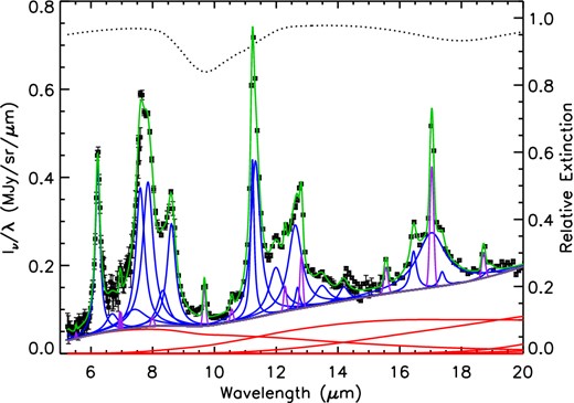
Detailed PAHFIT spectral decomposition of a 5-20 μm spectrum of the M82 outflow. The red solid lines represent the thermal dust continuum components, and the thick grey line shows the total (dust+stellar) continuum. Blue peaks set above the total continuum are PAH features, while the violet peaks are unresolved atomic and molecular spectral lines. A fully mixed dust extinction model is used (shape indicated by the dotted black line at the top), with the relative extinction given on the axis at right. The solid green line is the full fitted model, overlaid on the observed flux intensities and uncertainties.
![Maps of the continuum-subtracted total PAH emission between 5 and 14 μm (upper left), the [Ne ii]12.8 μm emission (upper right), total H2 S(1)–S(3) emission (lower left) and total [Ne iii]15.6 μm (lower right). The maps are clipped at 2σ level in all cases. The white radial strip in the bottom two panels are regions that have been masked out due to scattered light in the LL2 module, which affects the H2 S(1) and [Ne iii]15.6 μm line maps.](https://oup.silverchair-cdn.com/oup/backfile/Content_public/Journal/mnras/451/3/10.1093/mnras/stv1101/2/m_stv1101fig3.jpeg?Expires=1750348894&Signature=3oy5r5pz28NmdRVBNacIzJs6rXALNvIXtbogvbyaStuXWNMJREkArootKlCXLyRIKrGBdpVNWd13mES2g9qKwFLamFPdvv8b5XcMPWBtPyGpbBdGFUDErnuSybSAIP9wwGtLLZ9v5gfvM-zVgCFHP7X7w8saTdO9N~~d9Xd7LDUY9-zAS5Cm6dMSb~L-6AtanhWJvunhMO1cvSoXSKKvtVxP~4LsLg7oSHG6hUqFrZGqNNDm6Mfy35RuIQb8AoWRD8n51kkKKM4bv0LDjKHorJqJm16Dnvvp3tYsZWOYVAjeQre2COmExQ8aZmftZ7gQ~w6Y5Y~mADU~5lHq3FzoRw__&Key-Pair-Id=APKAIE5G5CRDK6RD3PGA)
Maps of the continuum-subtracted total PAH emission between 5 and 14 μm (upper left), the [Ne ii]12.8 μm emission (upper right), total H2 S(1)–S(3) emission (lower left) and total [Ne iii]15.6 μm (lower right). The maps are clipped at 2σ level in all cases. The white radial strip in the bottom two panels are regions that have been masked out due to scattered light in the LL2 module, which affects the H2 S(1) and [Ne iii]15.6 μm line maps.
3 RESULTS
3.1 Morphology of the dust, ionized gas and warm H2 emission
In Fig. 3 we present the total PAH emission map calculated by summing over all the PAH bands between 5 and 14 μm, the [Ne ii]12.8 μm flux map derived from the SL data cubes, the total H2 map derived from the SL and LL2 cubes, and the [Ne iii]15.6 μm emission map. We find widespread emission with significant structure in all of the line maps. To the north, both PAH and [Ne ii] exhibit two prominent, broad radial filaments. To the south, the PAH map shows a complex structure with a bubble, or loop. This loop is also seen in the [Ne ii] map. The overall morphologies of the warm H2 and Hα are generally very similar, as seen in the NIR by Veilleux et al. (2009). Maps of the cold molecular gas made in CO (J = 1–0) by Salak et al. (2013) are at lower spatial resolution, but also show extended, extraplanar gas.
We can study the physical properties of the ionized gas and PAHs by mapping the ratios between ionized lines such as [Ne iii]/[Ne ii] and between the different PAH bands. If the ionized gas is photoionized, the Ne line ratio is sensitive to the hardness of the radiation field and the ionization parameter. The Ne ratios observed in the outflow are standard values for the hardness of the radiation field found in starburst galaxies. The ratio of the 6.2, 7.7 and 11.3 μm PAH features can be used to estimate the ionization state and the size of the small dust grains (e.g. Draine & Li 2001). Even the overall absence of PAH emission may be related to the ionization state of the gas since we do not expect gas emitting strongly in [Ne iii] to show much PAH emission, as the small grains are easily destroyed by energetic photons (e.g. Engelbracht et al. 2006; Madden et al. 2006; Wu et al. 2006). The 11.3 μm/7.7 μm ratio is high when PAHs are more neutral and larger, while the 6.2 μm/7.7 μm PAH ratio is high when PAH grains are smaller. However, we caution that variations in the PAH line ratios are also influenced by the structural properties and elemental abundances in small particles giving rise to the PAH features (e.g. Yamagishi et al. 2012).
In Fig. 4, we present maps of the PAH 11.3/7.7 and 6.2/7.7 ratios, the H2/PAH ratio and the [Ne iii]/[Ne ii] ratio. The H2/PAH ratio map was produced using a H2 [S(1)–S(3)] total flux map and PAH (7.7 + 8.6 μm) flux map. Although there is a great deal of structure in the PAH ratio maps, the general trend is that the 11.3/7.7 and the 6.2/7.7 ratios increase as we move away from the starburst disc. The PAH 11.3/7.7 is enhanced by a factor of ∼4 and the PAH 6.2/7.7 is enhanced by a factor of ∼3 at the northern edge of the outflow compared to the regions near the centre of the starburst disc. There is an enhancement of the 11.3/7.7 and 6.2/7.7 ratios by ∼2 in the southeast edges of the outflow.
![Maps of the PAH 11.3/7.7 ratio (upper left), PAH 6.2/7.7 (upper right), H2[S(1)–S(3)]/PAH(7.7 + 8.6 μm) (lower left) and [Ne iii]/[Ne ii] (lower right). All maps have been clipped at the 3σ surface brightness level. The white radial strip in the bottom two panels are regions that have been masked out due to scattered light in the LL2 module, which affects the H2S(1) and [Ne iii] lines. The circles represent the selected regions where the spectra in Section 5 were extracted and analysed. The fluxes are presented in Tables 1 and 2 (see Section 2 for details).](https://oup.silverchair-cdn.com/oup/backfile/Content_public/Journal/mnras/451/3/10.1093/mnras/stv1101/2/m_stv1101fig4.jpeg?Expires=1750348894&Signature=IGIM1nICrrv8qSkIx424z0u9jpMR57MIYs3t6S4WX3m6M~ntcWg71A4EO1qsPa5aDj3h95zEHPobxN9QibyeekgN1NOEhVI6G-GcZfUfb4IWhkbEkuaJ-6IWrkL3raQeu6asxjX7hKmI2GI3pKkVFEi8RuRz7zNirKjSopERTewR6dqJD3-jvMdzCTPozHXg2gkZXC4bJVSdtuQTlRbErLhG29xxtzocKW-yNRMOTGj-w8FnnOuJXdHHRdPJHcQmWCX8gZX7TCOXfHu27pF2EpyDUhzWq9xK1Nu6KuPx~2blBqi4qfOTunTzsaC7-VfuJQyPzPMhkb-fYMnXdRDSBw__&Key-Pair-Id=APKAIE5G5CRDK6RD3PGA)
Maps of the PAH 11.3/7.7 ratio (upper left), PAH 6.2/7.7 (upper right), H2[S(1)–S(3)]/PAH(7.7 + 8.6 μm) (lower left) and [Ne iii]/[Ne ii] (lower right). All maps have been clipped at the 3σ surface brightness level. The white radial strip in the bottom two panels are regions that have been masked out due to scattered light in the LL2 module, which affects the H2S(1) and [Ne iii] lines. The circles represent the selected regions where the spectra in Section 5 were extracted and analysed. The fluxes are presented in Tables 1 and 2 (see Section 2 for details).
The H2/PAH ratio varies between 0.01 and 1, and the [Ne iii]/[Ne ii] ratio varies between 0.2 and 0.9. In the region between the PAH emission ‘fingers’ (as particularly evident in the Northern outflow region in Fig. 3), both maps show an enhancement of the ratio.
In Fig. 4, we also mark the 12 regions from which we have extracted 5-20 μm spectra and performed multitemperature fits to the H2 lines. We show these spectra in Fig. 5. These regions were chosen to represent the full range of H2/PAH ratios and to approximately sample the full spatial extent of the outflow. For comparison, we also show an integrated spectrum of the centre of M82 (Fig. 5; Beirão et al. 2008), which we use as a reference. In addition to the 12 regions, we also show a composite spectrum of the entire IRS map in Fig. 5. We measure the fluxes of the PAH features between 5 and 14 μm, the fine-structure lines [Ne ii] and [Ne iii], and the rotational excitation lines of H2 from S(0) to S(3) and present the results in Tables 1 and 2. Regions 1, 5, 6, 7 and 9 are the most similar to the reference spectrum in slope and the relative strength of PAH features, which is not surprising since they are located close to the centre. PAHs are also strong in regions 3, 8, 10, 11 and 12, but their spectrum also exhibits a flatter continuum, probably indicating the presence of colder dust. Region 3 is the most distant from the central starburst and it has the weakest PAH emission. Region 4 exhibits a flat continuum, but a comparatively strong PAH 11.3 μm feature.

PAH band and ionic line fluxes (in units of 10−16 Wm−2) and ratios. The regions for the extracted spectra are shown in Fig. 3 and described in the text.
| Region | 6.2 μm | 7.7 μm | 8.6 μm | 11.3 μm | 17 μm | PAH 6.2-12.6 μm | 6.2/7.7 | 11.3/7.7 | [Ne ii] | [Ne iii] |
|---|---|---|---|---|---|---|---|---|---|---|
| 1 | 7.12 | 23.31 | 4.19 | 6.44 | 3.52 | 44.58 | 0.305 | 0.151 | 3.62 | 1.36 |
| 2 | 1.86 | 3.31 | 1.28 | 2.56 | 0.920 | 9.93 | 0.562 | 0.278 | 2.60 | 0.966 |
| 3 | 1.01 | 2.58 | 0.526 | 1.12 | 0.751 | 5.987 | 0.391 | 0.291 | 1.27 | 0.550 |
| 4 | 0.811 | 4.76 | 0.895 | 2.65 | 1.76 | 10.876 | 0.170 | 0.370 | 0.536 | 0.893 |
| 5 | 12.53 | 40.41 | 8.93 | 13.86 | 8.32 | 84.05 | 0.310 | 0.206 | 2.17 | 5.38 |
| 6 | 7.30 | 22.03 | 6.04 | 10.65 | 7.94 | 53.96 | 0.331 | 0.360 | 2.79 | 4.18 |
| 7 | 9.39 | 29.26 | 6.61 | 11.43 | 7.47 | 64.16 | 0.321 | 0.255 | 6.06 | 3.44 |
| 8 | 349.6 | 1167.7 | 254.3 | 397.7 | 282.6 | 2451.9 | 0.299 | 0.242 | 339.3 | 89.4 |
| 9 | 741.9 | 2783.7 | 513.5 | 668.9 | 254.3 | 4962.3 | 0.261 | 0.091 | 568.0 | 83.1 |
| 10 | 10.3 | 37.6 | 82.7 | 18.3 | 10.7 | 159.6 | 0.274 | 0.285 | 5.43 | 2.57 |
| 11 | 30.9 | 105.7 | 22.2 | 37.0 | 21.3 | 217.1 | 0.292 | 0.202 | 30.2 | 9.91 |
| 12 | 8.22 | 27.2 | 7.55 | 15.0 | 9.40 | 67.37 | 0.302 | 0.346 | 9.37 | 4.17 |
H2 line fluxes (in units of 10−17 Wm−2) and ratios. ‘Total’ denotes the sum of all emission in the maps.
| Region | H2 S(0) | H2 S(1) | H2 S(2) | H2 S(3) | H2 S(1) – S(3) |
|---|---|---|---|---|---|
| 1 | <0.313 | 4.13 ± 0.12 | 0.840 ± 0.142 | 1.70 ± 0.14 | 6.67 |
| 2 | – | 4.35 ± 0.15 | 0.784 ± 0.173 | 3.94 ± 0.10 | 9.07 |
| 3 | <0.169 | 2.81 ± 0.07 | 0.517 ± 0.267 | 1.68 ± 0.23 | 5.01 |
| 4 | <1.45 | 6.68 ± 0.14 | 1.74 ± 0.16 | 3.17 ± 0.14 | 11.6 |
| 5 | <0.991 | 14.3 ± 0.2 | 3.93 ± 0.24 | 8.74 ± 0.41 | 27.0 |
| 6 | <2.81 | 9.68 ± 0.26 | 6.24 ± 0.55 | 2.05 ± 0.18 | 18.0 |
| 7 | <1.25 | 8.87 ± 0.14 | 2.37 ± 0.14 | 4.79 ± 0.20 | 16.0 |
| 8 | <48.7 | 37.8 ± 0.6 | 32.2 ± 0.4 | 83.4 ± 0.7 | 153.4 |
| 9 | – | 179.8 ± 0.8 | 84.6 ± 0.3 | 108.4 ± 0.3 | 372.8 |
| 10 | <0.528 | 23.9 ± 0.2 | 5.73 ± 0.11 | 119.0 ± 3.0 | 148.6 |
| 11 | <5.51 | 31.7 ± 0.2 | 10.4 ± 0.1 | 16.6 ± 0.1 | 58.7 |
| 12 | <0.613 | 8.85 ± 0.12 | 2.50 ± 0.12 | 4.94 ± 0.21 | 16.3 |
| Total | <253.9 | 1171.5 ± 3.2 | 455.1 ± 2.7 | 1010.0 ± 5.6 | 2636.6 |
As we have seen in the maps, the spectra show strong variations of the H2/PAH ratios between the regions. The H2S(1) line is very prominent in the spectrum of Region 3 compared to the PAH bands, while in the regions close to the disc, such as Regions 7 and 9, this line is much fainter compared to the PAH features. Indeed, using the values in Tables 1 and 2, we calculate in Region 3 a very high H2/PAH ∼ 0.08, while in Region 9, H2/PAH ∼ 0.01.
In Fig. 6, we present a plot of the PAH 11.3/7.7 ratio as a function of the 6.2/7.7 PAH ratio. The range of 6.2/7.7 PAH ratios in the outflow is much larger and the values are, on average, smaller than the disc. The outflow exhibits 6.2/7.7 and 11.3/7.7 ratios ranging between ∼0.2 and 0.4. On average, the bulk of the superwind shows larger, more ionized grains than in the starburst disc, although there are regions where the ratios overlap. As an example of the different PAH ratios found in the outflow, we present in the upper-right corner of Fig. 6, two spectra from different regions of the outflow, and an average spectrum of the disc. In general, the outflow has stronger 17 μm PAH and H2 emission than the SB disc, and the spectrum in the region 2 kpc north of the disc (the blue spectrum shown in Fig. 6) has higher 17 μm feature and H2 S(1) flux, indicating the prevalence of larger PAH grains and enhanced H2 emission further away from the disc. In summary, we see a much larger range in the PAH ratios in the outflow than is seen in the starburst disc. The average spectrum of the wind has smaller 6.2/7.7 ratios and larger 11.3/7.7 ratios than the average spectrum of the starburst, suggesting the grains may be larger and more ionized, on average, than those in the starburst disc.
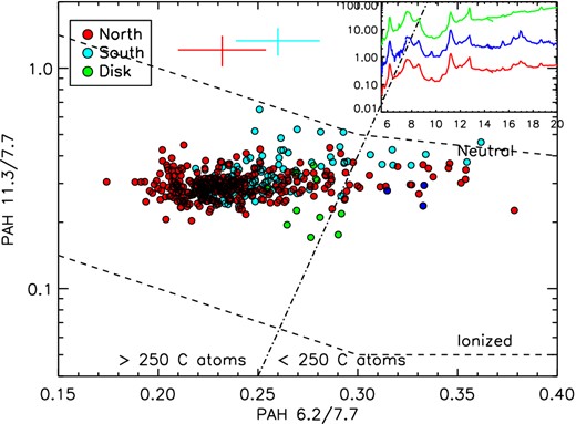
Plot of the PAH ratio 11.3/7.7 as a function of 6.2/7.7 for 10 arcsec × 10 arcsec regions in the outflow. Red represents the northern outflow, cyan the southern outflow and green represents the central 1 kpc in M82 from Beirão et al. (2008). The dashed lines represent neutral and ionized PAHs from Draine & Li (2001). The dot–dashed line represent the PAH ratio values for a PAH grain of 250 carbon atoms. The red and cyan crosses represent typical uncertainties in the north and southern outflows. The three spectra on the upper-right corner are derived from different regions in the outflow (in units of MJy sr−1). The blue spectrum is derived from a region 2 kpc north of the disc and is represented by the blue data points, the red spectrum is an average spectrum of the whole northern outflow, and the green spectrum the average spectrum of the central region.
3.2 H2/PAH variations in the M82 wind
In Fig. 7, we plot the variation of H2S(1)–S(3)/PAH7.7 + 8.6 μm as a function of [Ne ii] surface brightness. Since the [Ne ii] emission arises predominantly from the starburst disc, this traces the relative H2 and PAH emission as a function of distance from the starburst. This ratio has been previously used by Ogle et al. (2010) and Guillard et al. (2012) to show the relative importance of the UV versus mechanical heating of the gas. We can see that the H2/PAH ratio decreases with increasing [Ne ii] flux. The vast majority of the mapped regions lie well above the values seen in star-forming galaxies in the local Universe (the dashed lines; see Roussel et al. 2007). The H2/PAH ratio values span two orders-of-magnitude, 0.01–1. Most of the M82 wind points have H2/PAH between 0.01 and 0.10, but ∼4 per cent have extreme values, H2/PAH >0.5. The fact that the H2/PAH ratios seen in the wind are well above those seen in the SB disc, the normal galaxies observed by Roussel et al. (2007), and PDR models of Guillard et al. (2012, see section 4) suggests that the H2 is not solely excited by stellar radiation from the starburst.
![Plot of the H2 S(1)–S(3)/PAH (7.7 + 8.6 μm) as a function of the [Ne ii] surface brightness. Each data point represents a 10 arcsec × 10 arcsec region. Red points are the northern outflow, cyan the southern outflow, and green the central 1 kpc of M82 from Beirão et al. (2008). The dashed line and the dash–dotted lines represent the average and the 1σ variation, respectively, of the H2 S(1)–S(3)/PAH (7.7 + 8.6 μm) ratio in the star-forming galaxy sample of Roussel et al. (2007). The dot–dashed line represents the upper limit in the H2 S(1)–S(3)/PAH (7.7 + 8.6 μm) ratio predicted by PDR models (Guillard et al. 2012). The error bar in red represent typical uncertainties in the northern outflow, while the typical uncertainties in the data for the southern outflow region are smaller than the points.](https://oup.silverchair-cdn.com/oup/backfile/Content_public/Journal/mnras/451/3/10.1093/mnras/stv1101/2/m_stv1101fig7.jpeg?Expires=1750348894&Signature=OY7WAF7l5HlgGEyz-ja7Q~CBUf-YPJYnvIqhElWL441msgZwGaT13y6GHB~PcVuWkTkP3h1iNj0TZ1aUOgV-zLzu3KDlKELq31CZ5JmmIxwI0VUcE5ngkG5O2gYLi28-AAfw5e6sRz4oTCvcTsB0QokTld2jThgenn23r28YMA0IZaqt9qr4sPG5qPsyuvja4bBdJAmSfUGbSDVjWZLlXkX6t5ExNp5RCd1KPzD1wg-Kk09Dtnf5pS-ZqlpiWQEI0KmD7qhzE1t-IFHUOTj3en88~R4pdOEQoMMRgBLt7LDfSq~UC0yMrIitGKKXb03KkdO-gjp82z4KUvvSnjKDEg__&Key-Pair-Id=APKAIE5G5CRDK6RD3PGA)
Plot of the H2 S(1)–S(3)/PAH (7.7 + 8.6 μm) as a function of the [Ne ii] surface brightness. Each data point represents a 10 arcsec × 10 arcsec region. Red points are the northern outflow, cyan the southern outflow, and green the central 1 kpc of M82 from Beirão et al. (2008). The dashed line and the dash–dotted lines represent the average and the 1σ variation, respectively, of the H2 S(1)–S(3)/PAH (7.7 + 8.6 μm) ratio in the star-forming galaxy sample of Roussel et al. (2007). The dot–dashed line represents the upper limit in the H2 S(1)–S(3)/PAH (7.7 + 8.6 μm) ratio predicted by PDR models (Guillard et al. 2012). The error bar in red represent typical uncertainties in the northern outflow, while the typical uncertainties in the data for the southern outflow region are smaller than the points.
We can also investigate possible correlations of the H2/PAH ratio with diagnostics of the atomic gas and the size and ionization state of the grains. In Fig. 8, we show H2/PAH as a function of the PAH 11.3/7.7 ratio, the PAH 6.2/7.7 ratio, the H2 S(3)/S(1) ratio, and the [Ne iii]/[Ne ii] ratio. We see that in the disc the H2/PAH ratio increases with increasing PAH 11.3/7.7 ratio. While the trend of increasing H2/PAH in the wind is similar to that seen in the disc, the wind values extend to much larger values of both 11.3/7.7 PAH and H2/PAH than seen in the starburst. The scatter to high H2/PAH and a much larger range in the 6.2/7.7 ratio is seen in the upper-right panel of Fig. 8 as well. In the lower left, we observe an anticorrelation between H2/PAH and S(3)/S(1) in the disc as warmer gas has lower H2/PAH. The wind points seem consistent with this trend but the uncertainties are large. This general lack of very warm molecular gas and high H2/PAH ratios in the wind may be a function of inability of the MIR diagnostic features to probe the hottest gas. The [Ne iii]/[Ne ii] also increases with H2/PAH in the disc, and the wind points to the North seem consistent with the trend, but clearly there are many wind points in a few regions in the northern outflow which have much higher H2/PAH ratios than seen in the disc at a given [Ne iii]/[Ne ii] value.
![Plot of the H2 S(3)–S(1)/PAH (7.7 + 8.6 μm) as a function of PAH 11.3/7.7 (upper left), PAH 6.2/7.7 (upper right), H2 S(3)/S(1) (lower left) and [Ne iii]/[Ne ii] (lower right). Each data point represents a region of 10 arcsec × 10 arcsec in extent. Red points are the northern outflow, cyan the southern outflow, and green the central 1 kpc of M82 from Beirão et al. (2008). The error bars represent typical uncertainties in the northern (red) and southern (cyan) outflows. The dashed lines represent the average and the 1σ variation of the H2 S(1)–S(3)/PAH (7.7 + 8.6 μm) ratio in the star-forming galaxy sample of Roussel et al. (2007). The dot–dashed line represents the upper limit in the H2 S(1)–S(3)/PAH (7.7 + 8.6 μm) ratio predicted by PDR models (Guillard et al. 2012).](https://oup.silverchair-cdn.com/oup/backfile/Content_public/Journal/mnras/451/3/10.1093/mnras/stv1101/2/m_stv1101fig8.jpeg?Expires=1750348894&Signature=fsaZxOV52ln~d0mdzukSc6V7fQ9uv7vL2hGdXEAFEDfT7-BkyIvaPZyRom5ZM0emzYgxziQ~jBw4yaavekdbEDCD9wyC6WnPBx~f8QKeB63BU~5VOeL3Vczk2eZJQd~uZmdd8Fzb-afhbcgXBJtmBAYhz0vWZIfJl2IHycOM8w6C0PUMR7CivNQpUHFP-wvpr5JNdej0hmKsbOgpof-hwxYcQGHY9JsqO-IZHBpZ0fbdrrsiUYArvZOXSUYv6Xxsk-DvzQ4vG-SVaxYvBGg2Jts8Qb79zBp8BjQix16Mn3pg8lhL~oRw7bpAp2d0PlR3hxF6tm~0sDJDoisIgLUmbw__&Key-Pair-Id=APKAIE5G5CRDK6RD3PGA)
Plot of the H2 S(3)–S(1)/PAH (7.7 + 8.6 μm) as a function of PAH 11.3/7.7 (upper left), PAH 6.2/7.7 (upper right), H2 S(3)/S(1) (lower left) and [Ne iii]/[Ne ii] (lower right). Each data point represents a region of 10 arcsec × 10 arcsec in extent. Red points are the northern outflow, cyan the southern outflow, and green the central 1 kpc of M82 from Beirão et al. (2008). The error bars represent typical uncertainties in the northern (red) and southern (cyan) outflows. The dashed lines represent the average and the 1σ variation of the H2 S(1)–S(3)/PAH (7.7 + 8.6 μm) ratio in the star-forming galaxy sample of Roussel et al. (2007). The dot–dashed line represents the upper limit in the H2 S(1)–S(3)/PAH (7.7 + 8.6 μm) ratio predicted by PDR models (Guillard et al. 2012).
To further help us understand what drives the variations of the H2/PAH flux ratios, we present maps of H2/[Ne ii] and PAH/[Ne ii] in Fig. 9. In general, the regions with high H2/PAH correspond to high PAH/[Ne ii], suggesting that it is not simply a decreasing PAH that causes the rise in H2/PAH off the plane of M82. Only in the northern edge of the map do we see a lower PAH/[Ne ii] ratio, which might indicate reduced PAH heating efficiency. It is important to note, however, that while the PAH/[Ne ii] ratio does change by factors of a few across the map, this is much less than the variation observed in H2/PAH. Therefore the latter cannot be solely explained by a change in the strength of the PAH emission alone.
![Maps of the H2S(1)–S(3)/[Ne ii] ratio (left), PAH5-17 μm/[Ne ii] (right). H2 is the sum of the S(1), S(2), and S(3) H2 line fluxes and PAH5-17 μm is the sum of the fluxes of all PAH features be- tween ∼5 and 17 μm. All maps have been clipped at the 3σ surface brightness level. The white radial strip in the bottom two panels are regions that have been masked out due to scattered light in the LL2 module, as in Figs 3 and 4.](https://oup.silverchair-cdn.com/oup/backfile/Content_public/Journal/mnras/451/3/10.1093/mnras/stv1101/2/m_stv1101fig9.jpeg?Expires=1750348894&Signature=kZBtyqrbhJtRSAO4q4OWYztnLPLsrO-UNj4jcsqIudw1N88X-tdLI-bA8KxeHMkkod7X~36Jtrl9UXv0R03hvhgKsRiB-9C8v2UCgGCbDaG9LYaPt85z5sjsazP98gC4D~1-yzrQ1wRhMristtpH3rlgy1LiRxvHiZK1cjfMI71vaQ0h4VNGNP~3Pu1jXMsxmSc5RQejQs84-GYbEUZGJbjtx1whkS6~UDgxOUlaxCFymvhci0TtEoPpPqt4RYs-JLZ~1iWoawMzFmaBZ87owyJHAYkn-hplgxJqVaZyHaqTJpm3ZctjchTas3H1goLT-Fc~8UwQscfhJ6Eci57luA__&Key-Pair-Id=APKAIE5G5CRDK6RD3PGA)
Maps of the H2S(1)–S(3)/[Ne ii] ratio (left), PAH5-17 μm/[Ne ii] (right). H2 is the sum of the S(1), S(2), and S(3) H2 line fluxes and PAH5-17 μm is the sum of the fluxes of all PAH features be- tween ∼5 and 17 μm. All maps have been clipped at the 3σ surface brightness level. The white radial strip in the bottom two panels are regions that have been masked out due to scattered light in the LL2 module, as in Figs 3 and 4.
3.3 H2 masses and temperatures
With the rotational H2 emission line fluxes in Table 2, we can estimate the gas temperature, column density, and mass distributions, assuming that the ortho/para ratio is in local thermal equilibrium (LTE). In Fig. 10, we plot the excitation diagrams for all regions, except 2 and 9, which did not have sufficient signal-to-noise for fitting the data with these sorts of models. Using the Boltzmann equation, we fit the H2 lines with two components, each with different temperatures. We then derive the total column density, H2 temperatures and mass distributions. In fitting the data we set the minimum allowed temperature to 100 K and treated every upper limit as a 3σ detection. The S(1) line is the line with the highest signal-to-noise. Therefore, when we remove the S(0) line as a detection, we obtain essentially the same results.
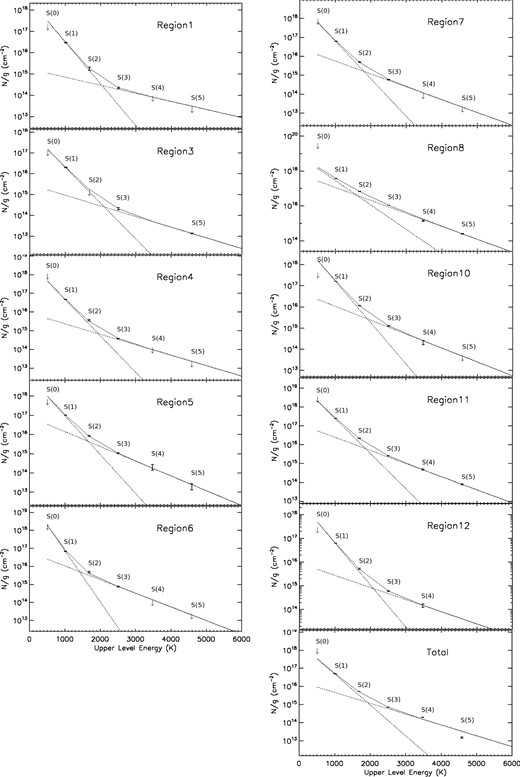
H2 excitation diagrams of most selected regions. The dotted lines show a two-temperature LTE fit of the data. The upper limits of the H2 lines represent a 3σ noise level at the corresponding line.
The diagrams for Regions 1, 3, 4, 5, 7 and 11 look very similar in shape, derived from very similar temperatures for each component. In Region 8, both components have similar temperatures, while in Region 10, there is a large difference in temperature between the two components. We note that Regions 8 and 10 have the most discrepant S(0) upper limits relative to the other fits, making the mass estimates particularly uncertain. In Table 3, we present the properties of the warm H2 gas in these regions of interest. In all the regions the temperature of the warmer component is above 500 K, especially warm when compared with typical star-forming regions (e.g. Roussel et al. 2007). The column density of the bulk of the warm H2 gas ranges by a factor of ∼30. The mass ratio between the warmer and colder component varies between 0.0003 and 0.02, with the lowest value observed in Region 8 and the highest in Region 1. The region with the most luminous H2 emission is Region 8, where the warmer component accounts for ∼95 per cent of the luminosity, whereas the next most luminous region, 11, the colder component accounts for ∼65 per cent of the luminosity.
H2 Temperature model parameters. ‘Total’ denotes the sum of all selected regions.
| Regions | T(K) | Ortho/Para | N(H2) | M(H2) | L(H2) |
|---|---|---|---|---|---|
| ×1019 cm−2 | ×104 M⊙ | ×104 L⊙ | |||
| Region1 | 210. ± 18. | 2.883 | 2.12 | 4.28 ± 1.47 | 1.43 |
| 1094. ± 208. | 3.000 | 0.05 | 0.0107 ± 0.0036 | 1.83 | |
| Region3 | 240 ± 54 | 2.945 | 0.838 | 12.9 ± 10.1 | 7.91 |
| 819 ± 126 | 3.000 | 0.007 | 0.113 ± 0.087 | 7.90 | |
| Region4 | 236. ± 14. | 2.940 | 2.07 | 4.19 ± 0.82 | 2.26 |
| 831. ± 124. | 3.000 | 0.0128 | 0.03 ± 0.01 | 1.84 | |
| Region5 | 206. ± 17. | 2.8871 | 6.77 | 13.7 ± 4.1 | 4.32 |
| 549. ± 54. | 3.000 | 0.132 | 0.27 ± 0.11 | 4.37 | |
| Region6 | 166. ± 21. | 2.653 | 13.5 | 27.3 ± 18.2 | 3.25 |
| 593. ± 56. | 3.000 | 0.086 | 0.152 ± 0.052 | 3.30 | |
| Region7 | 224. ± 12. | 2.917 | 3.30 | 6.66 ± 1.17 | 2.96 |
| 657. ± 75. | 3.000 | 0.0382 | 0.0771 ± 0.0297 | 2.68 | |
| Region8 | 324. ± 12. | 2.994 | 5.32 | 10.7 ± 0.6 | 64.0 |
| 595. ± 13. | 3.000 | 0.80 | 1.6 ± 0.2 | 3.6 | |
| Region10 | 218. ± 6. | 2.913 | 9.5 | 19.2 ± 1.7 | 33.0 |
| 637. ± 62. | 3.000 | 0.091 | 0.18 ± 0.06 | 5.2 | |
| Region11 | 233. ± 3. | 2.934 | 11.4 | 23.0 ± 0.81 | 11.8 |
| 623. ± 14. | 3.000 | 0.02 | 0.39 ± 0.03 | 10.1 | |
| Region12 | 241. ± 10. | 2.946 | 2.61 | 5.28 ± 0.666 | 3.17 |
| 816. ± 157. | 3.000 | 0.02 | 0.042 ± 0.002 | 3.09 | |
| Total | 272 ± 2 | 2.976 | 1.39 | 476 ± 7.66 | 463 |
| 854 ± 18 | 3.000 | 0.023 | 7.67 ± 0.42 | 640 |
We also integrated the emission over the entire observed nebula surrounding M82 and measured the line fluxes, which are included in Table 2. The total warm H2 mass derived from the integrated emission is ∼4.8 × 10⁶ M⊙. For completeness, we note that Veilleux et al. (2009) finds a mass of H2 at a temperature T>1000 K (thus hotter than our ‘hot’ gas) of 1.2 × 10⁴ M⊙, based on NIR observations. The relatively low mass is not surprising since the NIR ro-vibrational lines are probing very high excitation gas which emits very efficiently in these lines. The mass of warm molecular gas in the wind that we are detecting with the IRS is thus more than a factor of 100 more than is estimated from the NIR line maps. We have also estimated the H2 masses from fitting the H2 line fluxes with molecular shock models (see Section 4.3).
Considering a cold molecular gas mass of ∼109 M⊙ (Walter et al. 2002; Salak et al. 2013), we calculate a ratio of warm to cold molecular gas in the outflow of about 0.01. Therefore the warm molecular gas we measure here is a relatively minor component of the total molecular mass in the ISM. Care must be taken when making this comparison as the emission regions for the CO and H2 do not overlap completely. In fact, the most extended CO emission is only within a few arcminutes of the plane and much less extended (Walter et al. 2002; Salak et al. 2013), although new studies trace the CO-emitting gas to larger distances (Leroy et al., in preparation). However, we note that most of the estimated mass for the warm molecular gas in our observations also comes from regions which lie close to the disc (and likely the base of the wind).
4 DISCUSSION
4.1 H2 heating processes
In the scenario of thermal excitation of H2, three mechanisms dominate the heating: (1) UV radiation from starburst, (2) X-rays from the starburst and wind, and/or (3) shocks induced by the outflow. Following Ogle et al. (2010), we use the H2-to-PAH luminosity ratio to investigate the contribution of UV photons to the total heating of the H2 gas in the outflow. In starburst galaxies like M82, we expect the H2 emission to be predominantly powered by UV radiation from young stars but undoubtedly, processes such as low-velocity shocks and turbulent dissipation contribute to the H2 emission. It should also be noted that H2/PAH ratios on the order of 0.01 have also been seen from translucent clouds in the cold, diffuse ISM of the Milky Way, which are thought to be excited by UV photons (Ingalls et al. 2011).
There is a clear offset of the wind points from those in the SB disc in terms of H2, PAH and ionized atomic emission (Figs 7, 8, and 9). The data in regions of the outflowing gas show a large range in both [Ne iii]/[Ne ii] and H2/PAH, but are clearly offset to higher H2/PAH at a given [Ne iii]/[Ne ii] ratio compared to regions within the SB disc, suggesting an additional excitation mechanism at work. In fact, models suggest that the large values of the H2/PAH ratios observed in some regions (>0.1) cannot be explained by photoionization (Guillard et al. 2012).
The H2 gas could be indirectly excited by X-rays emitted from the expanding bubble of hot and tenuous gas generated by the intense star formation within M82 (Begelman & Cioffi 1989), high-velocity shocks in the entrained gas, X-rays due to inverse Compton scattering of IR photons. In M82, the X-ray emission covers approximately the same region as the optical emission line filaments (Watson, Stanger & Griffiths 1984; Shopbell & Bland-Hawthorn 1998) and radio emission (Seaquist & Odegard 1991). For example, the high H2/PAH in the northern tip ∼5 kpc from the disc, appears to be associated with a region with X-ray emission (Fig. 11).
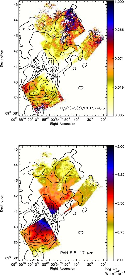
Image of the H2/PAH (top) and total PAH flux (5.2-17 μm) (bottom), overlaid with contours from soft (0.3–1.6 keV) X-ray emission map of M82 (Strickland & Heckman 2009).
We can use the total H2S(1)–S(3) luminosity and the total X-ray luminosity in the outflow to calculate the H2-to-X-ray luminosity ratio (Stevens, Read & Bravo-Guerrero 2003). The H to H2 transition can occur at relatively low column densities, NH ≈1021 cm−2. At such low columns, even relatively soft X-rays can penetrate. Our estimates for the M82 outflow are L(H2S(0) − S(3))/LX(2–10 keV) ∼ 1 (Stevens et al. 2003) and L(H2S(0) − S(3))/LX(0.2 − 4keV) ∼ 0.5 (Watson et al. 1984; Strickland & Heckman 2007), over the northern and southern IRS map. Using XDR models (e.g. Maloney, Hollenbach & Tielens 1996) we can estimate whether the H2 line emission could be powered by X-ray heating, following the procedure described in Ogle et al. (2010). In these models, 30–40 per cent of the absorbed X-ray flux goes into gas heating via photoelectrons, and the cooling by H2 rotational lines in XDR models is ∼2 per cent of the total gas cooling for a gas temperature of 200 K. At this temperature, the ratio of the first four rotational lines to the total rotational line luminosity is L(H2 0–0 S(0)–S(3))/ L(H2) = 0.6. Combining the above factors, we estimate a maximum H2 to X-ray luminosity ratio of L (H2 0–0 S(0)–S(3))/LX (2–10 keV) <0.01 (Guillard et al. 2012b). This upper limit on the H2-to-X-ray luminosity is conservative because it assumes that all the X-ray flux is absorbed by the molecular gas, which is likely not the case (since the medium in which X-rays propagate is inhomogeneous). Therefore, we conclude that X-rays are not the dominant source of heating of the H2 gas in the M82 wind, since the observed ratios are well above those found in XDR models. This is also seen in some extreme environments, such as powerful radio galaxies, where H2/PAH ∼0.5–1 and the H2/X-ray ratio also exceeds that expected from XDRs alone (Ogle et al. 2010).
Ambient gas clouds heated by the mechanical energy of the wind and dense shell fragments from the wind bubble carried along by the wind are the two main sources of X-ray emission in the wind (Strickland, Ponman & Stevens 1997). In Fig. 11, we show the contours of soft X-ray emission from the outflow of M82 overlaid on the H2/PAH and total (5-17 μm) PAH maps. The X-ray and PAH maps show a remarkable correlation, particularly in the southern part of the bi-conical outflow, although both maps are projections of the true 3D structure and the precise locations of the hot gas and dust grains are unknown. Moreover, there are regions of high surface brightness X-ray emission with relatively little PAH emission (in the north along the outer wind axis). We also see that the middle lobe of X-ray emission in the northern outflow, at about 5 kpc from the disc, appears related to the increase of H2/PAH7.7 + 8.6 μm surface brightness. The morphology of H2/PAH closely resembles the morphology of the H2 (2.12 μm)/PAH maps in Veilleux et al. (2009). The regions where H2/PAH > 0.1 correspond to regions where H2 (2.12 μm)/PAH > 0.003.
While there is a reasonable spatial correlation between the surface brightness distribution of the soft X-ray and H2 emission, a correlation is apparent between soft X-rays surface brightness and H2/PAH ratio distributions only in high surface brightness X-ray emitting regions. There are several possibilities why this might be so, but the most obvious is that both the X-ray and H2 emission are fundamentally powered by the same mechanism, namely, the very hot plasma that is acting as the ‘piston’ driving the wind and heating clouds entrained in the wind. However, the warm H2 and hot X-ray emitting plasma should not be co-spatial on small scales, and instead the H2 is likely seen in projection against the hot wind, along the edges of the cone in dense knots of gas, heated by shocks (see below). Such a situation would also arise in gas with a wide range of densities or through changes as individual clouds are shredded as they are accelerated by the action of the piston (Cooper et al. 2008). This is also shown by the strong correlation between the X-rays and the PAH emission (Fig. 11b), especially in the Southern wind. As the PAHs and H2 molecules cannot be expected to survive within the 106–107 K X-ray emitting plasma, it is most likely that they lie along the edges of this phase of the outflow. So while the power source is likely the same, the two emission regions, not surprisingly, represent different physical regions and gas states being impacted by the driving very hot plasma (Strickland & Heckman 2007).
4.2 The velocities and kinetic energy of the molecular gas
Kinematics of the gas can be used to determine if the different gas phases observed in the outflowing wind are related. If the observed kinematics of the warm molecular gas as probed by the H2 rotational lines is similar to that of the cold molecular gas as probed by the CO lines, the IR atomic neutral and ionized emission lines, or the lines of the warm ionized medium, then this might suggest a direct physical relationship between these phases.
Salak et al. (2013) derived a velocity of 160 km s−1 for the CO(1–0) emitting gas for the northern outflow region. However, the farthest extent of the CO emission is only about 1 arcmin north of the disc of M82, while the IRS map extends to 4 arcmin. The velocity derived by Salak et al. (2013) is not very different from the velocities in the neutral and ionized atomic gas in the infrared within the inner wind region <1 arcmin from the disc (Contursi et al. 2013). If we restrict ourselves to the inner wind region within a few arcminutes of the plane of M82, the velocities in the warm ionized gas are only a few 100 km s−1 or less within a couple of arcminutes of the disc of M82 (Shopbell & Bland-Hawthorn 1998). These velocities are consistent with those observed in IR neutral and ionized atomic lines (Contursi et al. 2013). However, farther out of the plane of M82, much higher outflow velocities (∼600–800 km s−1) are observed in Hα for the outflow in M82 (Shopbell & Bland-Hawthorn 1998). Line splitting is observed in both the CO and Hα with similar velocities (Walter et al. 2002), making the association between the cold molecular gas and the warm ionized gas stronger (cf. Shopbell & Bland-Hawthorn 1998; Salak et al. 2013).
Such a direct relationship would be consistent with a picture where the emission we observe in the extended outflow of M82 is mainly from entrained and swept-up clouds that are predominately shock-heated by a high ram-pressure, hot plasma generated within the starburst region. If we envision the regions of warm H2 emission as being the areas in the clouds that are shock-heated by the expanding plasma, we would expect these phases to co-exist with the warm ionized gas (Heckman et al. 1990) and the cold/warm molecular gas.
Assuming that the velocity of the warm H2 is similar to the deprojected velocity of the cold molecular gas derived by Salak et al. (2013), we can calculate its total kinetic energy as |$E_K=0.5\times M_{{\rm H}_2}v_{{\rm outflow}}^2\sim 5.9\times 10^{53}$| erg for |$M_{{\rm H}_2}\sim 4.8\times 10^6 \,\mathrm{M}_{{\odot }}$| and voutflow=160 km s−1. Our estimates are considerably higher than those of Veilleux et al. (2009) because both their mass estimates are a factor of 500 less and they assumed a velocity of 100 km s−1 for the warm molecular emission. However, they are smaller compared to those estimated for the cold molecular and warm ionized medium. Salak et al. (2013) estimate that the kinetic energy of the wind in the cold molecular gas is ≈1–4 × 1056 erg. Walter et al. (2002) estimate a kinetic energy of ≈3 × 1055 erg, but they do not map the CO distribution out to large distances from the disc compared to Salak et al. (2013).
4.3 H2 supersonic turbulent heating and shock models
The hot plasma driving the outflow will likely transfer part of its ram and thermal pressure to swept-up and entrained dense molecular gas by driving shocks and by turbulent mixing between hot and cold gas (see Guillard et al. 2009). To model such shocks, we use a grid of stationary shock models computed with an updated version of the Lesaffre et al. (2013) code to derive the physical shock parameters that explain the H2 line ratios. Our initial conditions are that the gas is diffuse, magnetized with a pre-shock magnetic field of intensity |$B[\mu G] = \sqrt{{\rm n}_{\rm H}[\rm cm^{-3}]}$|, and irradiated with a radiation field of G0 = 1 in Habing units. As the ‘Habing field’ would photodissociate the H2, we assume some self-shielding. In the models, we integrate the extinction along the model from the pre-shock, and we take into account the shielding and self-shielding, which is parametrized in the photodissociation reaction rates of H2 and CO (Lesaffre et al. 2013). At a density of 104 cm−3, the ionization fraction in the pre-shock gas is 6 × 10⁻⁸. This matches approximately our estimate of the ionization fraction of 10−7 at 10 kpc from the X-ray source. We fit the H2 line fluxes observed in the different regions with one shock or a combination of two shock velocities depending on how many H2 lines are detected, for three different pre-shock densities: nH = 102, 103 and 104 cm−3, [see Guillard et al. (2009) for details of the method]. The results of these fits are shown in Fig. 12, where we present the H2 excitation diagrams for the best velocity combinations (lowest χ2), and for the intermediate pre-shock density of nH = 103 cm−3. We present in Table 4 the results of the shock models for each region and the integrated spectrum (labelled ‘Total’). The total gas mass derived from the shock models is |$M_{H_2}=1.7\times 10^7 \,\mathrm{M}_{{\odot }}$|, which results in an estimate of the kinetic energy of EK ∼ 2 × 1054 erg. This is a factor of 3 higher than the estimates calculated in the temperature diagrams of Fig. 10. This difference arises due to the fact that we are integrating the post-shock temperature profile down to 50 K (where the H2 mid-IR lines start to emit), and because LTE is not assumed in the shock models. Our estimates of the total warm gas mass agree with previous studies using Herschel Spire-FTS (Kamenetzky et al. 2012).
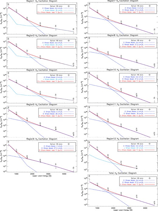
Shock excitation diagrams of most selected regions in the outflow. The best-fitting models for either J- (light blue) or C-shocks (dark blue) or a combination of each are indicated in the legend to each panel (see text for details). The sum of or the individual the best-fitting models is shown as a solid red line. The level populations of the various rotational levels of the (0–0) H2 lines are indicated by plus signs if they are detection or downward pointing arrows for upper limits and are labelled as S(1), S(2), S(3), S(4), and S(5).
H2 Shock Model Parameters. ‘Total’ denotes the sum of all selected regions.
| Regions | vshock | Mflow | tcool | M(H2) | Type |
|---|---|---|---|---|---|
| km s−1 | M⊙ yr−1 | ×103 yr | ×104 M⊙ | ||
| Region1 | 5.5 | 42 ± 3.1 | 1.6 | 6.8 ± 0.5 | C |
| 35.0 | 16 ± 1.4 | 3.4 | 5.4 ± 0.47 | J | |
| Region3 | 5.5 | 210 ± 35 | 1.6 | 34 ± 5.6 | C |
| 33.0 | 150 ± 11 | 3.2 | 48 ± 3.5 | J | |
| Region4 | 6.0 | 48 ± 6.1 | 1.6 | 7.6 ± 0.96 | C |
| 35.0 | 16 ± 2.4 | 3.4 | 5.5 ± 0.83 | J | |
| Region5 | 5.0 | 200 ± 12 | 1.6 | 33 ± 2.0 | C |
| 20.0 | 1.9 ± 0.14 | 2.1 | 0.41 ± 0.03 | C | |
| Region6 | 4.0 | 1200 ± 200 | 1.7 | 200 ± 33 | C |
| 21.5 | 1.3 ± 0.31 | 2.1 | 0.27 ± 0.06 | C | |
| Region7 | 5.0 | 130 ± 32 | 1.6 | 21 ± 5.2 | C |
| 21.5 | 0.97 ± 0.14 | 2.1 | 0.2 ± 0.029 | C | |
| Region8 | 5.5 | 400 ± 91 | 1.6 | 64 ± 15 | C |
| 21.5 | 17 ± 4.4 | 2.1 | 3.6 ± 0.93 | C | |
| Region10 | 5.5 | 210 ± 40 | 1.6 | 33 ± 6.3 | C |
| 21.5 | 1.5 ± 0.24 | 2.1 | 0.31 ± 0.05 | C | |
| Region11 | 5.0 | 500 ± 63 | 1.6 | 80 ± 10 | C |
| 18.0 | 6.2 ± 0.26 | 2.1 | 1.3 ± 0.05 | C | |
| Region12 | 5.5 | 84 ± 6.3 | 1.6 | 13 ± 0.98 | C |
| 22.0 | 33 ± 1.4 | 2.2 | 7.5 ± 0.32 | J | |
| Total | 5.5 | 10 000 ± 2100 | 1.6 | 1700 ± 360 | C |
| 21.5 | 180 ± 14 | 2.1 | 39 ± 3.1 | C |
For all regions, the best-fitting shock velocities are in the range 4–35 km s−1 (grid spans 3–40 km s−1; Table 4). These velocities are much lower than the estimated bulk outflow velocity (Lehnert et al. 1999). The regions show a range of best-fitting models, but typically the best-fitting pre-shock densities are nH = 100–1000 cm−3. Our modelling is not intended to be exhaustive, but to simply provide an estimate of the physical parameters in the warm molecular gas of the outflow.
At the range of preshock densities and magnetic field strengths considered, the C-shocks turn into J-shocks when the velocities are above ∼22 km s−1. For some regions the H2 line fluxes are reproduced by a combination of two C-shocks, in other regions the C-shocks (J-shocks) do not sufficiently populate the highest (lowest) energy levels. In those cases, we fit the H2 line fluxes by a combination of C- and J-shocks. The shocks travel through the clouds in ∼104–105 yr (for 1 pc clouds), which is much shorter than the dynamical time of the outflow [108 yr; Lehnert et al. (1999)]. Using the estimates of the warm molecular gas mass and the typical cooling time of the shocked H2 gas (tcool ∼ 104 yr for nH = 103 cm−3), we can estimate the mass flow of shocked gas, Mwarm/tcool ∼ 7.5 × 10⁶ M⊙/104 yr = 750 M⊙ yr−1, assuming that all the warm H2 is shock-heated. The dynamical time-scale of the H2-rich outflow is ∼4.5 kpc/200 km s−1 = 2.5 × 10⁷ yr implying a total mass of shocked gas ≈5 × 10⁹ M⊙. This estimate is likely to be an upper limit since the H2 gas may not extend over the whole outflow and because this assumes that the gas is only shocked once, which is highly unlikely. The high mass flow rate of shocked gas may require the reformation of H2 in the post-shocked gas (see Guillard et al. 2009, 2010) to prolong the survival time of the H2 gas in the outflow (e.g. Fragile et al. 2004). Clouds may also survive longer if the radiative cooling time is shorter than the time-scale necessary for the shocks to cross the cloud and the growth rate of Kelvin–Helmholtz instabilities (Cooper et al. 2008). Such processes would lower the total molecular mass required to explain the molecular emission from the outflow, although for the C-shocks considered here and even for many of the J-shocks as well, there is little destruction of H2. At any rate, the total gas mass that is shock heated is similar to that of the cold molecular gas. Therefore, the reservoir for the shocked gas is likely the cold molecular gas as probed through the CO emission from the wind.
4.4 PAH destruction
Since we see that the PAHs grains are on average larger and more ionized in the wind, it is natural to ask whether or not some of the enhanced H2/PAH could be done to a reduction in the PAH emission, rather than an enhancement of H2. The decrease in PAH flux is probably just due to a decrease of the radiation field, but there is also a change in the grain properties associated with the wind. The gradient of decrease in H2 emission is significantly lower than that of the PAH emission, suggesting an additional heating source for the H2 (see Section 3.2).
One of the ways PAH emission can decrease relative to H2 is PAH destruction. PAH grains can be destroyed either by hard radiation field, X-rays, or shocks. The EWs of the PAH features in starburst galaxies are observed to decrease sharply when [Ne iii]15.6 μm/[Ne ii]12.8 μm>2, where [Ne iii]/[Ne ii] traces the hardness of the radiation field. This has been interpreted as evidence of PAH destruction by intense radiation fields (Beirão et al. 2006; Wu et al. 2006). In M82, despite an increase of [Ne iii]15.6 μm/[Ne ii]12.8 μm in the outflow, in most of the outflow [Ne iii]15.6 μm/[Ne ii]12.8 μm remains less than 1. [Ne iii]15.6 μm/[Ne ii]12.8 μm∼1 indicates that there is hard (>40.96 eV) radiation present, but not enough to have an effect on the average PAH properties. Furthermore, only a small fraction of the gas in the M82 outflow is photoionized, and PAHs may survive in H i and H2 gas. PAH destruction is also very sensitive to the clumping factor of the gas. If the gas is dense and clumpy with relatively small volume filling factor and large covering fraction, the PAH grains will be shielded from the hard photons in the radiation field. So PAH destruction by hard photons is not likely to be the cause of the increase of H2/PAH in the wind.
PAH grains are rapidly destroyed in hot, X-ray emitting gas (Micelotta, Jones & Tielens 2010b). However, the presence of PAHs at large distances (10 kpc from the disc) in the outflow shows that they are protected in cooler phases of the gas, mostly in molecular gas. It is possible, however, that X-rays from the hot outflow fluid could destroy the PAH carriers, but the correlation between the X-ray emitting gas and the PAH maps, particularly in the Southern outflow, suggests that grain destruction by X-rays in the wind is not dominant.
Thermal collisions with very small and big grains can have a significant impact on the cooling of the hot gas ejected into the halo (Dwek, Rephaeli & Mather 1990). However, the impact of this cooling will generally be short lived since the cooling efficiency drops as the grain sputtering occurs in the hot gas (Guillard et al. 2009), unless the hot halo gas is constantly replenished with dusty gas. A physical dust cooling model is needed to fully assess whether thermal emission from collisionally heated dust in the hot plasma is a significant contribution to the gas cooling in the halo of M82, and whether this contribution changes as a function of the radius.
Another possible mechanism for PAH destruction is shocks. As seen in Fig. 12, the H2 emission that we see can be fitted with shock models having speeds of up to 40 km s−1. PAH destruction likely only becomes relevant for shock velocities >100 km s−1 (Micelotta, Jones & Tielens 2010a). It is unlikely that the low-velocity shocks that heat the molecular gas and enhance the H2 emission are also destroying the PAH grains, although we clearly see a change in the grain population. Similarly, Contursi et al. (2013) find that shocks do not dominate the [C ii] and [O i] emission in the wind. Overall, the enhancement in H2/PAH is likely caused by H2 excitation by shocks, although we cannot rule out a relatively small effect due to PAH destruction.
In dense molecular clouds, where the PAH destruction by shocks is less efficient, cosmic rays are the most efficient source of destruction of PAH molecules, mostly because of their bombardment by energetic ions (Micelotta, Jones & Tielens 2011). This is likely to play an important role in the M82 wind, because the intense star formation in M82 is likely to enhance the cosmic ray intensity by a factor of ≈5 compared to the Milky Way (Robitaille & Whitney 2010). Theoretical studies suggest that CRs can destroy PAHs in dense molecular clouds, but in these environments the heating will also be very inefficient, causing a reduction of PAH emission. Micelotta et al. (2011) showed that only PAHs with a number of carbon atoms greater than ≈250 have a survival lifetime greater than the circulation time-scale of the outflow (≈2 × 10⁸ yr). Thus, there may be a size-selection effect of PAHs in the outflow, which is roughly consistent with the size inferred from the band ratios (we mostly see PAH 6.2/7.7 < 0.3, meaning an average size greater than 250 carbon atoms, see Fig. 6), and cosmic rays are likely to play a role.
The calculations of Micelotta et al. (2010a) show that any PAH shocked at >100 km s−1 should be destroyed. To be re-formed in the post-shock gas, an efficient and fast re-formation process is needed. PAHs are a product of high-temperature chemistry involving abundant carbon bearing precursors such as CH4 and C2H2. In the cooled post-shock gas these precursor species are likely not very abundant. In the cold neutral medium, the global PAH coagulation time-scale is of the order of 100 Myr, much longer than the outflow dynamical time (Seok, Hirashita & Asano 2014). AKARI results from Yamagishi et al. (2012) suggest that very small grains still exist in the halo. Therefore, it is reasonable to assume that PAH are produced in the disc, carried up in the outflow, and ‘protected’ from fast shocks in the denser material. If molecular clouds are formed in the post-shock gas in the outflow, then there may be PAH coagulation over time-scales comparable to the outflow time (coagulation time-scales are of the order of a few Myr in molecular clouds), but it should be very small fraction of the volume, contrary to what is observed.
In conclusion, the enhancement of the H2/PAH is likely caused by H2 shock excitation, although we cannot rule out a relatively small effect due to PAH destruction.
5 CONCLUSION
We have mapped the northern and southern superwind in the nearby starburst galaxy M82 using the Spitzer-IRS. We find strong H2, PAH and Ne line emission that extends over nearly 5 arcmin above and below the plane of the galaxy, and have measured the variation of the H2/PAH, [Ne iii]/[Ne ii] and PAH feature ratios throughout the wind.
We estimate a total warm (100–500 K) molecular gas mass to be between ∼5 and 17 × 106 M⊙ and the total kinetic energy of the warm molecular outflow to be between ≈6 and 20 × 1053 erg assuming an outflow velocity voutflow = 160 km s−1. The warm molecular gas provides about 0.5–5 per cent of the kinetic energy – comparable to that observed in the atomic gas.
There are clear variations in the PAH band ratios throughout the wind. The 6.2/7.7 and 11.3/7.7 μm PAH band flux ratios, when compared to models, suggest a higher fraction of larger and/or more ionized PAHs in the wind compared to the starburst disc, especially in the northern part of the wind.
The warm molecular gas to PAH ratio (H2/PAH) is enhanced in the outflow by factors of 10–100 as compared to the starburst disc. This enhancement in the H2/PAH ratio does not seem to follow the trends with the ionization of the atomic gas (as measured with the [Ne iii]/[Ne ii] line flux ratio) seen in the starburst. Our results indicate that UV and X-ray emission are probably not the dominant excitation mechanisms of H2. Models suggest the observed values could be reproduced with slow C- and J-shocks (v < 40 km s−1) driven into dense molecular gas entrained in the outflow. Using a dynamical time-scale of the H2-rich outflow of about 107 yr results in an upper limit of 5 × 10⁹ M⊙ of molecular gas heated and shocked over the lifetime of the wind. Given the rate at which the gas must be shocked, the reservoir for this shocked gas is the cold molecular gas as observed in CO.
The emission from all of these phases is likely due to clouds entrained in and accelerated by the flow. They are being shock heated by the hot plasma with high ram pressure generated by the collective thermalization of stellar winds and supernova in the starburst region of M82. These clouds are multiphase and the variation in properties are likely due to a range of shock velocities which depend on the density of the pre-shocked gas which depend on the density of the pre-shocked gas.
We would like to thank an anonymous referee for a number of helpful comments which helped improve the quality of this paper. This work is based on observations made with the Spitzer Space Telescope, which was operated by the Jet Propulsion Laboratory, California Institute of Technology under a contract with NASA. Support for this work was provided by NASA through an award issued by JPL/Caltech. This work is dedicated to the memory of our friend and colleague, CE.
REFERENCES
