


Abstract
We extend the Kolmogorov–Smirnov (K–S) test to multiple dimensions by suggesting a |$\mathbb {R}^n \rightarrow [0,1]$| mapping based on the probability content of the highest probability density region of the reference distribution under consideration; this mapping reduces the problem back to the one-dimensional case to which the standard K–S test may be applied. The universal character of this mapping also allows us to introduce a simple, yet general, method for the validation of Bayesian posterior distributions of any dimensionality. This new approach goes beyond validating software implementations; it provides a sensitive test for all assumptions, explicit or implicit, that underlie the inference. In particular, the method assesses whether the inferred posterior distribution is a truthful representation of the actual constraints on the model parameters. We illustrate our multidimensional K–S test by applying it to a simple two-dimensional Gaussian toy problem, and demonstrate our method for posterior validation in the real-world astrophysical application of estimating the physical parameters of galaxy clusters parameters from their Sunyaev–Zel'dovich effect in microwave background data. In the latter example, we show that the method can validate the entire Bayesian inference process across a varied population of objects for which the derived posteriors are different in each case.
1 INTRODUCTION
The Kolmogorov–Smirnov (K–S) test and its close variants are the most widely accepted methods for testing whether a set of continuous sample data is drawn from a given probability distribution function (PDF) f(x) (see e.g. Press et al. 2007, ch. 14.3.3). The test is based on the computation of the maximum absolute distance D between the cumulative distribution functions (CDFs) of the data and of f(x). In particular, it has the advantage that, in the ‘null hypothesis’ that the data are indeed drawn from f(x), the distribution of D is both independent of the form of f(x) (i.e. the test is ‘distribution free’) and can be calculated, at least to a good approximation. Moreover, the test is invariant under reparametrizations of x. In its standard form, however, the K–S test is restricted to one-dimensional data, since a CDF can only be defined uniquely in the univariate case.
Considerable effort has been made to extend the K–S test to n-dimensional data sets, much of it building on the pioneering work of Peacock (1983), but this has proved very challenging precisely because a CDF is not well defined in more than one dimension. Working initially in two dimensions, Peacock's original insight was to replace the notion of a CDF with the integrated probability in each of the four natural quadrants around any given data point (xi, yi), and define the distance measure D as the maximum absolute difference (ranging both over data points and quadrants) of the corresponding integrated probabilities for the data and the theoretical distribution f(x, y). This basic idea can, in principle, be extended straightforwardly to higher dimensions (Gosset 1987), but in practice suffers from an exponential growth in complexity, since the number of independent integrated probabilities about any given data point is 2n − 1 in n-dimensions, although Fasano & Franceschini (1987) suggest an algorithm with better scaling. Perhaps a more notable deficit is that, in the null hypothesis, the distribution of D is not independent of the form of f(x, y), although Press et al. (2007) reassure us that extensive Monte Carlo simulations show the distribution of the two-dimensional D to be very nearly identical for even quite different distributions, provided they have the same correlation coefficient (Fasano & Franceschini 1987). Lopes, Hobson & Reid (2008) contain a review that ranks the performance of a range of different multidimensional K–S tests that are variants of Peacock's original proposal. A completely different approach to extending the K–S test to multiple dimensions was advanced by Justel, Peña & Zamar (1997) and employs the Rosenblatt transformation, which maps any distribution into the unit hypercube (Rosenblatt 1952). Despite this approach being formally sound, the authors report insurmountable difficulties when extending the test to more than two dimensions.
In this paper, we present a new proposal for extending the K–S test to multiple dimensions, which is free from the weaknesses discussed above and scales straightforwardly with the dimensionality of the data set. Our approach is to introduce the |$\mathbb {R}^n \rightarrow [0,1]$| mapping from any given (data) point |$\boldsymbol {x}_i$| in the n-dimensional parameter space to the probability mass ζ of the putative theoretical distribution |$f(\boldsymbol {x})$| contained within the highest probability density (HPD) region having |$\boldsymbol {x}_i$| on its boundary. This mapping has the convenient property that under the null hypothesis that the data are drawn from |$f(\boldsymbol {x})$|, the probability mass ζ is uniformly distributed in the range [0, 1], independently of the form of |$f(\boldsymbol {x})$|. The set of values {ζi} corresponding to the data points |$\lbrace \boldsymbol {x}_i\rbrace$| can then be compared with the uniform distribution in a standard one-dimensional K–S test (or one of its variants).
The ability to test the hypothesis that a set of data samples is drawn from some general n-dimensional probability distribution |$f(\boldsymbol {x})$| has an interesting application in the validation of Bayesian inference analyses (indeed this application provided our original motivation for seeking to extend the K–S test to multiple dimensions). Bayesian methods are now pervasive across all branches of science and engineering, from cognitive neuroscience (Doya et al. 2007) and machine learning (Bishop 2006) to spam filtering (Sahami et al. 1998) and geographic profiling (Collins, Gao & Carin 1999; Le Comber & Stevenson 2012). In precision cosmology, Bayesian inference is the main tool for setting constraints on cosmological parameters (Hinshaw et al. 2013; Planck Collaboration XVI 2014), but very few attempts have been made to assess whether the derived posterior probability distributions are a truthful representation of the actual parameter constraints one can infer from the data in the context of a given physical model. This lack of validation has been highlighted by several authors, with the strong dependence of the inference results on the priors being of particular concern (Efstathiou 2008; Linder & Miquel 2008). There have been attempts to address this issue, ranging from the approach of Cook, Gelman & Rubin (2006), which was designed with software validation solely in mind, to a method based on the inverse probability integral transform (Smirnov transform) applied to posterior distributions that extends to spaces of higher dimensionality via marginalization (Dorn, Oppermann & Enßlin 2013). Also, validation of the Bayesian source-finding algorithm of Carvalho et al. (2012) was performed in Planck Collaboration XXIX (2014), but only point estimates deduced from the posterior distributions were actually verified. Our method for addressing this problem is based on our applying our multidimensional extension of the K–S test to sets of Monte Carlo simulations of the data and the posterior distributions derived therefrom. In particular, it can take advantage of the fact that one may typically generate simulations that are of greater sophistication and realism than may be modelled in the inference process, and thus allows for a more thorough validation of the inference than has been possible with the methods developed previously. In particular, our validation procedure enables us to test all the assumptions made (explicitly or implicitly) in the inference process, such as the statistical description of the data, model assumptions and approximations, as well as the software implementation of the analysis. Moreover, we consider the full posterior distribution, regardless of its dimensionality and form, without the need to resort to marginalization, and thereby keeping intact its n-dimensional character.
This paper is organized as follows. Section 2 provides the mathematical background for our extension of the K–S test to multiple dimensions and Section 3 describes its application to the validation of Bayesian inference analyses. In Section 4.1 we apply our multidimensional K–S test to a simple toy problem, and in Section 4.2 we illustrate our Bayesian inference validation procedure by applying it to the real astronomical example of detecting and characterizing galaxy clusters in observations of the microwave sky through their Sunyaev–Zel'dovich (SZ) effect. We conclude in Section 5.
2 MULTIDIMENSIONAL K–S TEST
2.1 Classical one-dimensional K–S test and its variants
It is well known, however, that the K–S test is not equally sensitive over the entire range of the variable x, since under the null hypothesis the variance of |SN(x) − F(x)| is proportional to f(x)[1 − f(x)]. Consequently, the K–S test is most sensitive around the median point, where f(x) = 0.5, and less sensitive in the tails of the distribution. This makes the K–S test particularly sensitive to ‘shifts’ (in particular differences in the median), but less sensitive to differences in the dispersion, particularly if the median is similar. Two popular variants of the K–S test seek to remedy this shortcoming in different ways. Anderson & Darling (1952) suggest correcting for the effect by ‘stabilizing’ the statistic D using a weighting scheme based on the standard deviation of the null hypothesis, although the probability distribution of the resulting ‘distance’ statistic does not have a simple form. A more direct approach, proposed by Kuiper (1962), is to wrap the x-axis around into a circle (by identifying the points at x = ±∞) and define a new ‘distance’ statistic that is invariant under all reparametrizations on the circle. This guarantees equal sensitivity at all values of x and there exists a simple formula for the asymptotic distribution of the statistic. Clearly, this variant is ideally suited for distributions originally defined on a circle.
2.2 Highest probability density regions
To extend the K–S test (and its variants) to multiple dimensions, one must clearly replace the use of the CDF, since this is not uniquely defined in more than one dimension. In the univariate case, the CDF simply maps the value of the random variable x to the integrated probability under its PDF up to that x-value. This suggests that to accommodate multiple dimensions one should seek an alternative mapping, that is well defined in any dimensionality, from the multidimensional random variable |$\boldsymbol {x}$| to an associated integrated probability under |$f(\boldsymbol {x})$|. We therefore choose here to use the probability mass ζ contained within the HPD region having |$\boldsymbol {x}$| on its boundary.
HPDs are discussed by Box & Tiao (1992) as a general method for compressing the information contained within a probability distribution |$f(\boldsymbol {x})$| of arbitrary dimensional and form. Each HPD is uniquely defined by the amount of probability ζ it encloses and is constructed such that there exists no probability density value outside the HPD that is greater than any value contained within it. More formally, HPDζ is the region in |$\boldsymbol {x}$|-space defined by |$\Pr (\boldsymbol {x} \in \mbox{HPD}_\zeta )=\zeta$| and the requirement that if |$\boldsymbol {x}_1\in \mbox{HPD}_\zeta$| and |$\boldsymbol {x}_2\not\in \mbox{HPD}_\zeta$| then |$f(\boldsymbol {x}_1) \ge f(\boldsymbol {x}_2)$|. Fig. 1 provides a graphical illustration of the HPD definition in two dimensions.
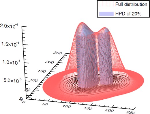
Illustration of the definition of the HPD region in a two-dimensional case. The unique HPD that encloses 20 per cent of the probability is shown. All the values that are contained within the HPD have higher probability densities than those that lie outside this region.
Some properties of HPD regions are summarized in Appendix A. In particular, we show that HPDζ is the region with smallest volume that encloses a total probability ζ; thus the HPD provides an elegant way of communicating inference results, since it corresponds to the smallest region of parameter space having a given level of (un)certainty ζ.
2.3 Pathological cases
Before continuing with the mathematical development, it is necessary to discuss some pathological cases that require further consideration. Such cases occur when there exist perfect ‘plateau’ regions of the parameter space over which |$f({\boldsymbol {x}})$| takes precisely the same value.
As a result, even if a set of data points |$\lbrace {\boldsymbol {x}}_i\rbrace$| is drawn from |$f({\boldsymbol {x}})$|, the corresponding values {ζi} will not be drawn from the standard uniform distribution U(0, 1). The extreme example is when |$f({\boldsymbol {x}})$| is the uniform distribution over the entire parameter space, in which case the mapping (7) yields the value ζi = 1 for every point |${\boldsymbol {x}}_i$| (in this case the entire contribution to ζ comes from the second integral on the RHS of equation 7, since the first one vanishes).
Fortunately, we can accommodate such pathological cases by using the fact that data points drawn from |$f({\boldsymbol {x}})$| are uniformly distributed within the perfect plateau regions. For such a set of data points, which exhibits complete spatial randomness, it is straightforward to show that, in N dimensions and ignoring edge effects, the CDF of the nearest neighbour Euclidean distance d is G(d) = 1 − exp [ − ρVN(d)], where |$V_N(d)=\pi ^{n/2}\text{d}^n/\Gamma (\frac{n}{2}+1)$| is the ‘volume’ of the N-ball of radius d (such that |$V_2(d)=\pi \text{d}^2$|, |$V_3(d) = \frac{4}{3}\pi \text{d}^3$|, etc.), and ρ is the expected number of data points per unit ‘volume’. Similarly, again ignoring edge effects, the CDF F(s) of the distance s from a randomly chosen location (not the location of a data point) in a perfect plateau region and the nearest data point has the same functional form as G(d). Most importantly, as described by van Lieshout & Baddeley (1996), one may remove edge effects by combining G(d) and F(s). In particular, provided the data points exhibit complete spatial randomness, the quantity J(d) ≡ [1 − G(d)]/[1 − F(d)] will equal unity for all d and does not suffer from edge effects.
2.4 Testing the null hypothesis
It is now a simple matter to define our multidimensional extension to the K–S test. Given a set of data points |$\lbrace {\boldsymbol {x}}_i\rbrace$|, we may test the null hypothesis that they are drawn from the reference distribution |$f({\boldsymbol {x}})$| as follows. First, we apply the mapping (4) (or the mapping 7 in pathological cases) to obtain the corresponding set of values {ζi}. Second, we simply use the standard one-dimensional K–S test (or one of its variants) to test the hypothesis that the values {ζi} are drawn from the standard normal distribution U(0, 1).
In this way, one inherits the advantages of the standard one-dimensional K–S test, while being able to accommodate multiple dimensions. In particular, since under the null hypothesis the set of values {ζi} are uniformly distributed independently of the form of |$f({\boldsymbol {x}})$|, our approach retains the property enjoyed by the one-dimensional K–S test of being distribution free; this contrasts with the method proposed by Peacock (1983).
We note that, once the {ζi} values have been obtained, one could test whether they are drawn from a uniform distribution using any standard one-dimensional test. For example, if one wished, one could bin the {ζi} values and use the chi-square test (see e.g. Press et al. 2007), although there is, of course, an arbitrariness in choosing the bins and an inevitable loss of information. For continuous one-dimensional data, such as the {ζi} values, the most generally accepted test is the K–S test (or one of its variants).
We also note that our approach may be applied even in the absence of an analytical form for |$f(\boldsymbol {x})$|, provided one has some (numerical) means for evaluating it at any given point |$\boldsymbol {x}$|. An important example is when one has only a set of samples known to be drawn from |$f(\boldsymbol {x})$|. In this case, one might evaluate |$f(\boldsymbol {x})$| at any given point using some kernel estimation method (say). If, however, one also knows the value of |$f(\boldsymbol {x})$| at each sample point, a more elegant approach is to estimate the probability mass ζi corresponding to each original (data) point |$\boldsymbol {x}_i$| by calculating the fraction of samples for which |$f(\boldsymbol {x}) \ge f(\boldsymbol {x}_i)$|.
2.5 Performing multiple simultaneous tests
The advantageous property that, under the null hypothesis, the derived set of values {ζi} are drawn from the standard uniform distribution U(0, 1), independently of the form of |$f(\boldsymbol {x})$|, allows us straightforwardly to perform multiple simultaneous tests as follows.
As an extreme example, this approach may even be used when one has just a single data point drawn from each reference distribution |$f_m({\boldsymbol {x}})$|, in which case it would be impossible to perform an individual test for each data point. We will make use of this capability in applying our method to the validation of Bayesian inference analyses in Section 3.
2.6 Reparametrization invariance
A common criticism of HPD regions is that they are not invariant under smooth reparametrizations (Lehmann & Romano 2006, section 5.7). In other words, if one performs a smooth change of variables |${\boldsymbol {x}} \rightarrow \boldsymbol {\theta } = \boldsymbol {\theta }({\boldsymbol {x}})$|, then in general |$\mbox{HPD}_\zeta (\boldsymbol {\theta }) \ne \boldsymbol {\theta }(\mbox{HPD}_\zeta ({\boldsymbol {x}}))$|, although the image |$\boldsymbol {\theta }(\mbox{HPD}_\zeta ({\boldsymbol {x}}))$| in |$\boldsymbol {\theta }$|-space of the |${\boldsymbol {x}}$|-space HPD region will still contain a probability mass ζ. This deficiency can be problematic for using HPD regions to summarize the properties of probability density functions, but it causes less difficulty here, since our only use of the HPD region is to define the mapping (4).
Suppose that a set of data points |$\lbrace {\boldsymbol {x}}_i\rbrace$| is drawn from |$f({\boldsymbol {x}})$| and is transformed into the set |$\lbrace \boldsymbol {\theta }_i\rbrace$|, which will be drawn from the corresponding PDF |$h(\boldsymbol {\theta })$| in the new variables. Applying an analogous mapping to equation (4) to the new data set |$\lbrace \boldsymbol {\theta }_i\rbrace$| will, in general, lead to a different set of values {ζi} to those derived from the original data |$\lbrace {\boldsymbol {x}}_i\rbrace$|. One may visualize this straightforwardly by considering any one of the data points |${\boldsymbol {x}}_i$|, for which |$f({\boldsymbol {x}}_i)=f_i$| (say), and the corresponding HPD region having |${\boldsymbol {x}}_i$| on its boundary, which is defined simply by the contour |$f({\boldsymbol {x}})=f_i$|. Performing a smooth mapping |${\boldsymbol {x}} \rightarrow \boldsymbol {\theta } = \boldsymbol {\theta }({\boldsymbol {x}})$|, the data point |${\boldsymbol {x}}_i$| will be transformed into |$\boldsymbol {\theta }_i$|, which will clearly lie within the image in |$\boldsymbol {\theta }$|-space of the |${\boldsymbol {x}}$|-space HPD, although not necessarily on its boundary. This image region will contain the same probability mass as the original x-space HPD, but it will in general not coincide with the HPD in |$\boldsymbol {\theta }$|-space having |$\boldsymbol {\theta }_i$| on its boundary, which may contain a different probability mass. Nonetheless, subject to the caveats above regarding pathological cases, the values {ζi} derived from the transformed data |$\lbrace \boldsymbol {\theta }_i\rbrace$| will still be uniformly distributed in the interval [0, 1], since this property does not depend on the form of the PDF under consideration.
This does not mean, however, that the significance of our multidimensional K–S test is invariant under reparametrizations. Under the alternative hypothesis that the data are not drawn from the reference distribution, the transformation |$\lbrace {\boldsymbol {x}}_i\rbrace \rightarrow \lbrace \boldsymbol {\theta }_i\rbrace$| may result in new derived values {ζi} that differ more significantly from the standard uniform distribution than the original set.
There exists the scope for adapting our approach, so that the significance of the test is reparametrization invariant, by replacing the HPD with an alternative mapping from the n-dimensional parameter space |${\boldsymbol {x}}$| to some other measure of integrated probability under |$f({\boldsymbol {x}})$|. One such possibility is to use the ‘intrinsic credible interval’ (ICI) proposed by Bernardo (2005), which has numerous desirable properties, including invariance under both reparametrization and marginalization. We have not pursued this approach here, however, since the definition of the ICI is rather complicated and its calculation often requires numerical integration. It also does not follow that the resulting mapping is distribution free. We therefore leave this as a topic for future work.
In the context of the validation of Bayesian inference analyses, however, in Section 3.3 we will discuss a method by which one may retain the use of the HPD and ensure that the values of {ζi} derived from the original and transformed data sets, respectively, are in fact identical under smooth reparametrizations. Thus, the significance of our resulting multidimensional K–S test will be similarly invariant in this case.
2.7 Iso-probability degeneracy
We conclude this section, by noting that, even when our test gives a ‘clean bill of health’ to a set of data points, it unfortunately does not guarantee immediately that those points were drawn from the reference distribution. The basic test described above provides only a necessary condition; for it to be sufficient (at least in the limit of a large number of data points) requires further refinement, which we now discuss.
To understand this limitation of our basic test, we note, as mentioned previously, that for the mapping (4) more than one point |$\boldsymbol {x}$| in the parameter space may map on to the same ζ-value. Indeed, given a point |$\boldsymbol {x}$|, the boundary of the corresponding HPD is an iso-probability surface, and any other point lying on this surface will naturally be mapped on to the same ζ-value. This constitutes the iso-probability degeneracy that is inherent to the mapping (4). Thus, for example, if one drew a set of data points |$\lbrace \boldsymbol {x}_i\rbrace$| from some PDF |$f(\boldsymbol {x})$|, and then moved each data point arbitrarily around its iso-probability surface, the derived {ζi}-values from the original and ‘transported’ set of data points would be identical, despite the latter set clearly no longer being drawn from |$f(\boldsymbol {x})$|. Thus, the basic test embodied by the mapping (4) is not consistent against all alternatives: it is possible for there to be two rather different multidimensional PDFs that are not distinguished by the test statistic, even in the limit of a large number of data points. As an extreme example, consider the two-dimensional unit circularly symmetric Gaussian distribution f(x, y) = (2π)− 1exp [ − (x2 + y2)/2] and the alternative distribution g(x, y) = δ(y)H(x)x exp (−x2/2), where δ(y) is the Dirac delta function and H(x) is the Heaviside step function. Our basic test cannot distinguish between these two distributions, since data points drawn from the latter can be obtained by moving each data point drawn from the former along its iso-probability contour to the positive x-axis.
There are, however, a number of ways in which this difficulty can be overcome. Most straightforwardly, one can extend the basic approach to include separate tests of each lower dimensional marginal of |$f(\boldsymbol {x})$| against the corresponding marginal data set. In a two-dimensional case, for example, one would also test, separately, the hypotheses that the one-dimensional data sets {xi} and {yi} are drawn from the corresponding reference distributions obtained by marginalization of f(x, y) over x and y, respectively. This would clearly very easily distinguish between the two example distributions f(x, y) and g(x, y) mentioned above.
![Illustration of the ‘jelly mould’ function $g(x,y) = \frac{1}{2\pi }\exp \left(-\frac{x^2+y^2}{2}\right) \left[1 + \sin (\pi x) \sin (\pi y)\right]$. A constant value of 0.1 has been added to help visualize the function.](https://oup.silverchair-cdn.com/oup/backfile/Content_public/Journal/mnras/451/3/10.1093/mnras/stv1110/2/m_stv1110fig2.jpeg?Expires=1750287259&Signature=IAJS5gUPMaaix-8QiVVR3ve~QWfXMMGfGNIwe6vuWJnoEhMKVAlT-wsBDg6rmODJOHLsfVZS4ez-v1djZyEPg3VpJOhEc9T7e2td7xba30gFDh7V5~~qVISM0NVELlxuejFgInTxBarwC9QboIQ9lx5kGwdIrCA4c2DbRAjmz5EEk~7FU3jeJnFH0MQPGz-M3EqhgrqAF~lRL0N3yytNpCYbIgY5sNfozQQhKQhs8CH7zkAITwTu-d0~ECpdR0NAJYueu3HkFXOBr5YS8UmfmrE7e9AcKgnuKJPicrUrL0OgPp48079fCzwo0oebOhnUZ-PLFi9lmFua~66IfbxE3Q__&Key-Pair-Id=APKAIE5G5CRDK6RD3PGA)
Illustration of the ‘jelly mould’ function |$g(x,y) = \frac{1}{2\pi }\exp \left(-\frac{x^2+y^2}{2}\right) \left[1 + \sin (\pi x) \sin (\pi y)\right]$|. A constant value of 0.1 has been added to help visualize the function.
Fig. 3 shows a demonstration of this test. Two sets of data points, each containing 100 000 samples, were drawn: one set from the two-dimensional unit circularly symmetric Gaussian distribution f(x, y), and the other from the ‘jelly mould’ distribution g(x, y) given in equation (10). Each set of samples was tested against the Gaussian reference distribution f(x, y). Owing to the iso-probability degeneracy, the basic test finds that each set of samples is consistent (at better than the nominal 5 per cent confidence level indicated by the dashed black line) with being drawn from the Gaussian distribution, as illustrated by the solid red and green lines in the figure. If, however, one instead uses the ziggurat approximation fZ(x, y; NB) to the Gaussian as the reference distribution, then one can easily distinguish between the two sets of samples. As shown by the red stars in Fig. 3, the samples from the Gaussian distribution pass the new test for large values of NB, but fail it for small NB, as the ziggurat approximation to the Gaussian becomes poorer. By contrast, as shown by the green diamonds, the samples from the jelly mould distribution g(x, y) fail the test for all values of NB. As an additional check, the blue circles in the figure show the probabilities obtained for a set of 100 000 samples drawn from the ziggurat approximation fZ(x, y; NB) itself; since this is the reference distribution, these samples should pass the test for all values of NB, as is indeed the case.

The K–S test probability that a set of samples is drawn from the two-dimensional unit circularly symmetric Gaussian reference distribution f(x, y). The solid red and greens lines show the probabilities obtained using our basic test on a set of 100 000 samples from the reference distribution f(x, y) and the jelly mould distribution g(x, y), respectively. The dashed black line shows the nominal 5 per cent probability level, constituting the pass/fail boundary of the test. The red stars show the probabilities obtained for the same set of samples from f(x, y) in the case where the reference distribution is instead the ‘ziggurat’ approximation fZ(x, y; NB) to the Gaussian, defined in equation (12), for several values of NB. The green diamonds show the corresponding probabilities obtained for the samples from the jelly mould g(x, y). The blue circles show the corresponding probabilities obtained for a set of 100 000 samples taken from the ‘ziggurat’ approximation fZ(x, y; NB) itself.
It should be noted that it is not possible to extend our basic test in the manner outlined above for the extreme case, described in Section 2.5, where one wishes to perform multiple simultaneous tests but one has just a single data point drawn from each reference distribution. This therefore precludes the application of the extended test described above to the validation of posterior distributions in Bayesian inference, which is discussed in Section 3.2. In this application, one is thus restricted to using our basic test, the passing of which provides only a necessary, but not sufficient, condition for the Bayesian analysis to be consistent. Indeed, for the remainder of this paper, we will consider only our basic test.
3 VALIDATION OF BAYESIAN INFERENCE ANALYSES
3.1 Bayesian inference
3.2 Validation of posterior distributions
Conditioned on the assumed model H (and background information I), all valid Bayesian inferential statements about the parameters |$\boldsymbol {\theta }$| are encapsulated in the posterior distribution |$\mathcal {P}(\boldsymbol {\theta })$|, which combines the information provided by the data and any other information about the parameters contained in the prior.
Nonetheless, as discussed in the Introduction, relatively little consideration has been given to assessing whether the derived posterior distribution is a truthful representation of the actual constraints on the parameters that one can infer from the data, in the context of a given model. The possibility that some difference might exist is the result of the almost inevitable need to use some approximate data model H in the inference process, at least in most real-world problems. More prosaically, such differences might also be the result of errors in the implementation.
Our proposed validation procedure for testing the assumptions made (explicitly or implicitly) in the inference process (as well as the software implementation) is to make use of the fact that one may typically generate simulations of greater sophistication and realism than the data model H assumed in the analysis. One may regard the simulations as representing some alternative, more realistic data model H′. Our approach is then to test whether the posterior distribution(s) obtained from the simulated data by assuming H are consistent with the simulations generated assuming H′.
It is worth noting that this procedure does not suffer from the usual complications associated with the number of degrees of freedom being reduced by the number of parameters that have been optimized. A pertinent example of this issue is provided by Lilliefors’ variant of the K–S test for the null hypothesis that a set of data points is drawn from a Gaussian distribution of unknown mean and variance (Lilliefors 1967). In this test, the mean and variance of the Gaussian reference distribution used in the K–S test are first estimated from the data points, with the result that the distribution of the K–S distance (equation 1) in this case is stochastically smaller than the usual K–S distribution (equation 2). By contrast, in applying the K–S test to the set of values {ζk} (k = 1, 2, …, Nd) defined in equation (15), no optimization of parameters has been performed. Rather, one has calculated the full posterior distribution |$\mathcal {P}_k(\boldsymbol {\theta })$| on the parameters for each simulated data set. If the Bayesian inference process is valid, then the true parameter values |$\boldsymbol {\theta }^{(k)}_\ast$| should simply be drawn from precisely this posterior distribution, which constitutes our null hypothesis.
It should be noted that our validation procedure as described here allows for the verification of the implementation and any simplifying assumptions of the data model used. It does not validate whether the simulated data model is consistent with reality. If one wishes to use this procedure for this purpose, then the reader should be aware that the number of degrees of freedom would be reduced, since then we would be using a distribution derived from the data to fit the data.
3.3 Reparametrization invariance
As discussed in Section 2.6, HPD regions are not reparametrization invariant,3 and as a result the significance of our multidimensional K–S test will also depend on the choice of parametrization in the data model. In the context of posterior distributions, however, Druilhet & Marin (2007) have suggested a simple, yet general, way to overcome this problem.
As pointed out by Druilhet & Marin (2007), another motivation for using the Jeffreys measure is that it is also a classical non-informative prior, which minimizes the asymptotic expected Kullback–Leibler distance between the prior and the posterior distributions, provided there are no nuisance parameters (Bernardo 1979). Thus, if no prior knowledge is available on the parameters |$\boldsymbol {\theta }$|, we may set |$\pi (\boldsymbol {\theta })$| to be uniform and identify the last two factors in equation (17) as the non-informative Jeffreys prior.
This result implies that the significance of our test is invariant to smooth reparametrization if non-informative priors are assigned to the parameters. If the priors assigned to any of the free parameters are informative, however, any important reparametrizations of the model should be considered separately.
3.4 Nuisance parameters and marginalization
It is often the case that the full parameter space is divided into parameters of interest and nuisance parameters; we will denote this by |$\boldsymbol {\theta }=(\boldsymbol {\theta }_\mathrm{i},\boldsymbol {\theta }_\mathrm{n})$|. So far we have assumed that the validation of the posterior distribution(s) is performed over the full parameter space |$\boldsymbol {\theta }$|, whereas in practice it may be preferable first to marginalize over the nuisance parameters |$\boldsymbol {\theta }_\mathrm{n}$| and then perform the validation only in the space of the parameters of interest |$\boldsymbol {\theta }_\mathrm{i}$|.
It is clear that the significance of our test will, in general, differ between validations performed in the spaces |$\boldsymbol {\theta }$| and |$\boldsymbol {\theta }_\mathrm{i}$|, respectively. More importantly, performing the validation after marginalizing over the nuisance parameters |$\boldsymbol {\theta }_\mathrm{n}$| is itself quite a subtle issue. Since the Jeffreys measure on |$\boldsymbol {\theta }$| does not distinguish between parameters of interest and nuisance parameters, if one simply marginalizes equation (17) over |$\boldsymbol {\theta }_\mathrm{n}$|, it does not follow that HPD regions derived from it in |$\boldsymbol {\theta }_\mathrm{i}$|-space are reparametrizaton invariant, i.e. |$\mbox{JHPD}_\zeta (\boldsymbol {\phi }_\mathrm{i}) \ne \boldsymbol {\phi }(\mbox{JHPD}_\zeta (\boldsymbol {\theta }_\mathrm{i}))$| in general.4
4 APPLICATIONS
We now illustrate the use of our multidimensional K–S test and its application to the validation of Bayesian inference analyses. In Section 4.1, we apply the multidimensional K–S test to the simple toy example of testing whether a set of two-dimensional data {xi, yi} are drawn from a given two-dimensional Gaussian reference distribution. In Section 4.2, we apply our related approach for validating posterior distributions to the real-world case of estimating the parameters of galaxy clusters through their SZ effect in the recently released Planck nominal mission microwave temperature maps of the sky (Planck Collaboration I 2014).
4.1 Multidimensional K–S test: toy problem
We illustrate our multidimensional K–S test by first applying it, separately, to four sets of 800 data points {xi, yi} (denoted by the red crosses in the left-hand panels of Figs 4–7, respectively) to test the hypothesis that each set is drawn from the two-dimensional Gaussian reference distribution f(x, y) indicated by the black 1–4σ contours in each figure. Although the first data set is indeed drawn from f(x, y), the remaining three data sets are drawn from two-dimensional Gaussian distributions that are rotated in the xy-plane by different angles relative to f(x, y). We use the term ‘correlation angle’ ψ to denote the angle measured anticlockwise from the y-axis of the first principal direction of the distribution from which each data set is drawn, whereas the ‘mismatch angle’ ψmis = ψ − ψref, where ψref = 30° is the correlation angle of the reference distribution f(x, y); these values are listed in Table 1.
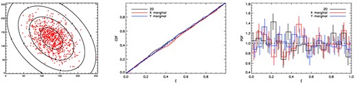
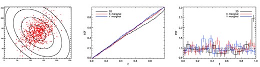
Left: the data points {xi, yi} (red crosses) and two-dimensional Gaussian reference distribution f(x, y) (black 1–4σ contours) to which the multidimensional K–S test is applied. In this case the data are drawn from the reference distribution, so that the ‘correlation angle’ ψ = 30° and ‘mismatch angle’ ψmis = 0°. Middle: the CDF of the standard uniform distribution (dot–dashed black line) and the empirical CDFs of the corresponding {ζi}-values for the full two-dimensional case (solid black line) and for the one-dimensional x- and y-marginals, respectively (red and blue solid lines). Right: the PDF of the standard uniform distribution (dashed black line) and the empirical PDFs of the corresponding {ζi}-values (constructing by dividing them into 20 bins) for the full two-dimensional case (solid black line) and for the one-dimensional x- and y-marginals, respectively (red and blue solid lines); the error bars denote the Poissonian uncertainty.
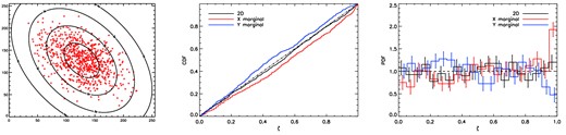
As in Fig. 4, but for ψ = 45° and ψmis = 15°.
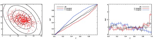
As in Fig. 4, but for ψ = 60° and ψmis = 30°.
As in Fig. 4, but for ψ = −30° and ψmis = −60°, so that the two-dimensional Gaussian from which the data are drawn is the reflection in the y-axis of the reference distribution; hence the one-dimensional marginals of the two distributions are identical.
The p-values for the null hypothesis, as obtained from our multidimensional K–S test applied to the data points (red crosses) and reference distribution (black contours) shown in the left-hand panels of Figs 4–7. In each case, the ‘correlation angle’ ψ is the angle, measured anticlockwise from the y-axis, of the first principal axis of the distribution from which the samples were actually drawn. The ‘mismatch angle’ ψmis = ψ − ψref, where ψref = 30° is the correlation angle of the assumed reference distribution. The p-values are given both for the full two-dimensional case, and for separate tests of the corresponding one-dimensional marginals in x and y, respectively. Also given, in parentheses, are the p-values obtained from the standard one-dimensional K–S test applied directly to the x- and y-marginals, respectively.
| ψ | 30° | 45° | 60° | −30° |
|---|---|---|---|---|
| ψmis | 0° | 15° | 30° | −60° |
| 2D | 0.27 | 0.59 | 6.6 × 10⁻³ | 1.4 × 10⁻⁶ |
| x marginal | 0.37 | 2.7 × 10⁻⁵ | 4.1 × 10⁻¹³ | 0.41 |
| (0.55) | (2.7 × 10⁻³) | (6.8 × 10⁻¹¹) | (0.93) | |
| y marginal | 0.41 | 1.7 × 10⁻³ | 4.0 × 10⁻¹⁸ | 0.51 |
| (0.10) | (1.4 × 10⁻⁴) | (3.9 × 10⁻²⁰) | (0.11) |
As mentioned in Section 3.4, the significance of our test will, in general, be different after marginalization over some parameters. Thus, in each of the four cases, it is of interest also to test, separately, the hypotheses that the one-dimensional data sets {xi} and {yi} are drawn from the corresponding Gaussian reference distributions obtained after marginalization of f(x, y) over x and y, respectively.
Since the marginal distributions are one-dimensional, it is also possible to compare directly the CDFs of the data sets {xi} and {yi} with those of the corresponding one-dimensional Gaussian reference marginal in a standard K–S test. We therefore also perform these tests in each of the four cases, in order to compare the resulting p-values with those obtained using our method.
4.1.1 Mismatch angle: 0°
Fig. 4 shows our nominal toy test example in which the data points are indeed drawn from the reference distribution. The middle panel of Fig. 4 shows the CDF of the corresponding {ζi} values obtained from the joint two-dimensional test (solid black line), and from the separate tests on the x- and y-marginals (red and blue solid lines). In all cases, the empirical CDF lies very close to that of the standard uniform distribution (dot–dashed black line), as one would expect. The resulting p-values derived from these tests are given in the second column of Table 1, and confirm that the data are consistent with being drawn from the reference distribution. We also list in parentheses the p-values obtained by applying the standard one-dimensional K–S test, separately, to the x- and y-marginals, which again are consistent with the null hypothesis.
For the purposes of illustration, in the right-hand panel of Fig. 4, we also plot the empirical PDFs of the {ζi}-values in each case, constructed by dividing the range [0, 1] into 20 equalwidth bins; the Poissonian error bars on each bin are also shown. As expected, these PDFs all appear consistent with the standard uniform distribution. Although this plot plays no part in deriving the significance of the test, it allows for a visual inspection of the PDFs. As we will see later, in the case of deviations from uniformity, this can provide useful clues as to the nature of the discrepancy.
4.1.2 Mismatch angle: 15°
We now consider the case where the two-dimensional Gaussian from which the data are actually drawn is rotated through an angle ψmis = 15° relative to the reference distribution, as shown in the left-hand panel of Fig. 5. The CDFs of the resulting {ζi}-values are shown in the middle panel for the two-dimensional case and the one-dimensional x- and y-marginals, respectively. In the two-dimensional case, the empirical CDF lies close to that of a uniform distribution, and the corresponding p-value obtained is p = 0.59 (see Table 1), which shows that the test is not sufficiently sensitive to rule out the null hypothesis. For the one-dimensional marginals, however, the CDFs do appear to differ significantly from that of the uniform distribution, and this is verified by the resulting p-values of 2.7 × 10⁻⁵ and 1.7 × 10⁻³, respectively. This shows the merit of performing the test both on the full joint distribution and on the marginal distributions. For comparison, the p-values obtained by applying the standard K–S test directly to the one-dimensional x- and y-marginals, respectively, are p = 2.7 × 10⁻³ and 1.4 × 10⁻⁴.
The empirical binned PDFs of the {ζi}-values plotted in the right-hand panel of Fig. 5 are easier to interpret that their CDFs, and provide more clues as to the nature of the discrepancy between the data and the reference distribution. In particular, the large excess in the final bin for the x-marginal and the corresponding decrement for the y-marginal are due to the non-zero ‘mismatch angle’ between the true and reference distributions; this results in the marginal distributions of the data in being too narrow in x and too broad in y, as compared to the marginals of the reference distribution.
4.1.3 Mismatch angle: 30°
Fig. 6 shows the results for the case in which the mismatch angle is increased to ψmis = 30°. The CDFs plotted in the middle panel are now all visibly discrepant from that of a uniform distribution. From Table 1, we see that this observation is confirmed by the very small p-values obtained in this case. Similarly tiny p-values, given in parentheses in the table, are also obtained when applying the standard one-dimensional K–S test directly to the x- and y-marginals. The empirical binned PDFs plotted in the right-hand panel exhibit similar behaviour to those obtained for ψmis = 15°, but are more exaggerated. In particular, for the x-marginal, relative to the uniform distribution there is now clear decrement in the PDF around ζ ∼ 0.2 and an excess near ζ ∼ 1, with the y-marginal exhibiting complementary behaviour. The behaviour of the x-marginal (y-marginal) clearly follows what one would if the spread of the data is greater (less) than the width of the reference distribution; if we had instead sampled the data from a distribution that was wider (narrower) than the reference distribution (i.e. by multiplying both eigenvalues of the reference covariance matrix by the same factor), rather than rotated with respect to it, then all the PDFs would have exhibited this pattern.
4.1.4 Mismatch angle: −60°
Fig. 7 shows the results for the case in which the distribution from which the data are sampled is the reflection in the y-axis of the reference distribution, resulting in ψmis = −60°. In this case the x-and y-marginals of the two distributions are identical. As expected, the CDFs for the two marginals, plotted in the middle panel, appear completely consistent with that of a uniform distribution, which is in agreement with the large p-values obtained in this case (see Table 1). For the two-dimensional case, however, the CDF is clearly discrepant, and the resulting p-value rules out the null hypothesis at extremely high significance. This shows, once again, the merit of testing for consistency both of the full joint distribution and its marginals. The PDF for the two-dimensional case, shown in the right-hand panel, again shows a clear excess near ζ ∼ 1, relative to the uniform distribution.
4.1.5 Comparison with theoretical expectation
In this simple toy example, one may in fact calculate straightforwardly the expected PDF of the ζ-variable for any given mismatch angle ψmis between the reference distribution and the true one from which the data are drawn. Each value of ζ specifies an HPD of the reference distribution that itself defines a region of the parameter space. If the probability content of the true distribution within this region is χ(ζ), then the PDF is simply p(ζ) = χ(ζ)/ζ. Fig. 8 shows the expected PDFs for the x- and y-marginals for three different mismatch angles ψmis, which clearly exhibit the behaviour we observed previously in Figs 5 and 6.
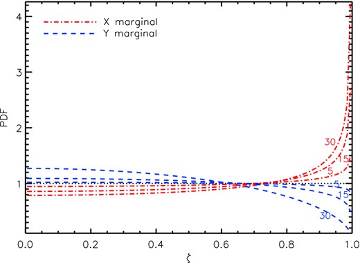
The expected PDF of the ζ-variable for the x-marginal (dot–dashed line) and y-marginal (blue dashed line) for mismatch angles of 5°, 15° and 30°.
We note that the sensitivity of our test in this toy example depends upon the maximum distance between the CDF of the ζ-values and that of a uniform distribution, and also on the number of data samples. It is clear that, for larger mismatch angles, fewer samples will be necessary to reject the null hypothesis at some required level of significance. Indeed, from Fig. 8, one may estimate the number of samples N required to obtain a given significance of when testing either the x- or y-marginal. For example, to reject the null hypothesis at a significance of 95 per cent, in the case of ψmis = 30°, one finds that N ∼ 130 for both the x- and y-marginals, whereas for ψmis = 5°, one requires N ∼ 2500 for the x-marginal and N ∼ 17 000 for the y-marginal.
4.1.6 Testing in many dimensions
So far we have demonstrated our multidimensional K–S test as applied to a toy model in two dimensions. Application to distributions with an arbitrary number of dimensions is straightforward and we demonstrate this here by extending the toy example to six dimensions. In this example, our six-dimensional Gaussian fiducial distribution has two discrepancies compared to the true distribution from which the data are drawn: in the first dimension the fiducial Gaussian σ is underestimated relative to the true σ by 30 per cent; in the second dimension, the mean of the fiducial distribution is translated by 0.5σ. The CDFs of the 1D marginals and the full 6D distribution, together with their p-values, are shown in Fig. 9. The marginals of dimensions one and two show a strong discrepancy, with p-values that robustly reject the null-hypothesis, as does the CDF of the full 6D distribution. The other dimensions are consistent with no discrepancy.
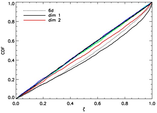
The CDFs of the {ζi}-values for an example in six dimensions. The full 6D case is shown by the dotted line, the marginal for dimension 1 (with a scale parameter underestimation) is shown by the black solid line, and the marginal for dimension 2 (with a mean translation) is shown by the red line. Each of these distributions is inconsistent with the uniform CDF, possessing a p-value <10−8. The remaining dimensions are consistent with the uniform CDF and possess p-values in the range 0.2–0.94.
4.1.7 Simultaneous test of multiple reference distributions
Returning to our two-dimensional toy example we now demonstrate the flexibility of our approach by performing a simultaneous test of multiple reference distributions, as discussed in Section 2.5. To this end, we generate simulated data as follows. For each data point, we draw a correlation angle ψ from a uniform distribution between 30° and 60°; this correlation angle is then used to define a reference distribution from which a single sample is drawn. The process is repeated 2400 times. This therefore corresponds to the extreme example, discussed in Section 2.5, in which just a single data point is drawn from each reference distribution.
Performing the simultaneous test on the full set of 2400 data points, as outlined in Section 2.5, produces the p-values listed in the second column of Table 2. As expected, these values clearly support the null hypothesis that each data point was drawn from its respective reference distribution. One may also straightforwardly perform the test on subsets of the data, with the division based on some given property of the corresponding reference distributions. To this end, Table 2 also shows the p-values for three subsets of the data for which the correlation angle ψ lies in the ranges indicated. Once again, all the p-values support the null hypothesis, as expected.
The p-values for the null hypothesis, as obtained from our multidimensional K–S test applied simultaneously to 2400 data points, where each one is drawn from a separate two-dimensional Gaussian reference distribution with a correlation angle ψ itself drawn from a uniform distribution between 30° and 60°. The p-values are given both for the full two-dimensional case, and for the x- and y-marginals, respectively. The second column lists the p-values for the full set of data points, and the columns 3–5 list the p-values for subsets of the data for which ψ lies in the ranges indicated.
| 30° ≤ ψ ≤ 60° | ψ < 40° | 40° ≤ ψ < 50° | 50° ≤ ψ | |
|---|---|---|---|---|
| 2D | 0.51 | 0.41 | 0.98 | 0.77 |
| x | 0.52 | 0.24 | 0.64 | 0.61 |
| y | 0.16 | 0.20 | 0.92 | 0.57 |
| 30° ≤ ψ ≤ 60° | ψ < 40° | 40° ≤ ψ < 50° | 50° ≤ ψ | |
|---|---|---|---|---|
| 2D | 0.51 | 0.41 | 0.98 | 0.77 |
| x | 0.52 | 0.24 | 0.64 | 0.61 |
| y | 0.16 | 0.20 | 0.92 | 0.57 |
To explore the sensitivity of our test, we also generate simulated data in which, for each data point, we introduce a mismatch between the correlation angle of the reference distribution and that of the distribution from which the sample is drawn. As previously, we draw the correlation angle ψref of the reference distribution uniformly between 30° and 60°, but we now draw the sample from a distribution with a correlation angle |$\psi =\psi _\mathrm{ref}+\frac{3}{2}\left(\psi _\mathrm{ref} -45^\circ \right)$|. We again performed the test separately on three subsets of the data for which the correlation angle ψref of the reference distribution lies in the ranges [30°, 40°], [40°, 50°] and [50°, 60°], respectively. For each of these subsets, it is easy to show that the mismatch angle ψmis = ψ − ψref is distributed uniformly in the ranges [−22| $_{.}^{\circ}$|5, −7| $_{.}^{\circ}$|5], [ − 7| $_{.}^{\circ}$|5, 7| $_{.}^{\circ}$|5] and [7| $_{.}^{\circ}$|5, 22| $_{.}^{\circ}$|5], respectively. Thus, the mean absolute mismatch angle is 15° for the first and third subsets, but zero for the second subset. The resulting p-values for these subsets are listed in Table 3, and follow a similar pattern to the case ψmis = 15° in Table 1, with the two-dimensional unable to reject the null hypothesis, but the x- and y-marginal cases ruling out the null hypothesis at extremely high significance for the first and third subsets. For the second subset, for which the mean mismatch angle is zero, the x- and y-marginal tests are consistent with the null hypothesis.
As in Table 2, but for the case in which the correlation angle ψref of the reference distribution is drawn uniformly between 30° and 60°, and the corresponding data point is drawn from a distribution with a correlation angle |$\psi =\psi _\mathrm{ref}+\frac{3}{2}\left(\psi _\mathrm{ref} -45^\circ \right)$|.
| ψref < 40° | 40° ≤ ψref < 50° | 50° ≤ ψref | |
|---|---|---|---|
| 2D | 0.12 | 0.71 | 0.30 |
| x | 1.1 × 10⁻⁶ | 0.49 | 1.9 × 10⁻² |
| y | 6.5 × 10⁻⁶ | 0.90 | 1.3 × 10⁻³ |
| ψref < 40° | 40° ≤ ψref < 50° | 50° ≤ ψref | |
|---|---|---|---|
| 2D | 0.12 | 0.71 | 0.30 |
| x | 1.1 × 10⁻⁶ | 0.49 | 1.9 × 10⁻² |
| y | 6.5 × 10⁻⁶ | 0.90 | 1.3 × 10⁻³ |
4.2 Validation of Bayesian inference: Planck SZ clusters
We now illustrate our method for the validation of posterior distributions derived from Bayesian inference analyses. We apply this approach to the subtle, real-world example of the estimation of cluster parameters via their SZ effect in microwave temperature maps of the sky produced by the Planck mission. For a description of the Planck maps and the details of the construction of the SZ likelihood, see Planck Collaboration I (2014), Planck Collaboration XXIX (2014) and references therein.
4.2.1 Cluster parametrization
In this application, we are again considering a two-dimensional problem, namely the validation of the derived posterior distribution(s) for scale-radius parameter θs and integrated Comptonization parameter Ytot of the galaxy cluster(s). Two further parameters defining position of the cluster centre are marginalized over, and several more model parameters are held at fixed values with δ-function priors. The most important of these fixed parameters are the those defining the spherically symmetric Generalized Navarro–Frenk–White (GNFW) profile used to model the variation of pressure with radius in the cluster (Nagai, Kravtsov & Vikhlinin 2007). Specifically, if rs is the scale-radius of the cluster, these parameters are (c500, γ, α, β), where c500 = r500/rs with r500 being the radius at which the mean density is 500 times the critical density at the cluster redshift, and γ, α and β describe the slopes of the pressure profile at r ≪ rs, r ∼ rs and r > rs, respectively. The parameters are fixed to the values (1.18, 0.31, 1.05, 5.49) of the ‘universal pressure profile’ (UPP) proposed by Arnaud et al. (2010).
4.2.2 Evaluation of the posterior distributions
In the analysis of Planck data, for each cluster the posterior distribution of its parameters is obtained using the PowellSnakes (PwS) algorithm (Carvalho et al. 2012). The marginalized two-dimensional posterior in (θs, Ytot)-space is evaluated on a high-resolution rectangular grid. The posteriors derived are typically complicated, non-Gaussian and vary between individual clusters, with different levels of correlation, skewness and flexion, as both the signal and noise changes.
In order to achieve a tractable inference, the Planck SZ likelihood used in these analyses necessarily makes a number of simplifying assumptions. As described above, the cluster model assumes that the pressure profile is well described by a spherically symmetric GNFW profile, with the same fixed shape parameters for all clusters; this may be a very poor approximation for some clusters. Aside from the cluster model, the analysis assumes the background emission in which the clusters are embedded is a realization of a homogeneous Gaussian process within the small patch of sky surrounding the cluster, whereas in reality foreground signals from Galactic emission (mostly dust) and infrared compact sources add a non-Gaussian and anisotropic component that dominates in certain areas of the sky. It is also assumed that the cluster signal is convolved at each observing frequency with a position-independent Gaussian beam, whereas in reality the effective beams are not symmetric and vary across the sky.
4.2.3 Validation of the posterior distributions
Our method to validate the posteriors makes use of the fact that one may generate simulations of the data that are often of (considerably) greater sophistication and realism than can be modelled in the inference process. In this application, the assumptions made by the Planck SZ likelihood clearly divide into those related to the model of the cluster itself and those associated with the background emission and observing process. We will concentrate here on the latter set of assumptions, but will return to the issue of the cluster model at the end of this section. Of course, our validation process also automatically provides a test of the software implementation of the inference analysis.
We generate our simulations as follows. The mass and redshift of the injected clusters are drawn from a Tinker mass function (Tinker et al. 2008) (assuming h = 0.7, σ8 = 0.8, Ωm = 0.3). The SZ parameters (Y500, θ500) are calculated using a Planck-derived scaling relation (Planck Collaboration XXIX 2014). We inject the simulated clusters (each having the GNFW profile with the fixed UPP shape parameters assumed in the analysis), convolved with the appropriate effective beams, into the real Planck sky maps. By doing so, we are thus testing all the assumptions and approximations (both explicit and implicit) made in the Planck SZ likelihood that are not associated with the cluster model itself. PwS is then run in detection mode to produce a catalogue of realistic detected clusters. The injected values of the SZ observables (Ytot, θs) are calculated from the injected (Y500, θ500) using the injected GNFW profile.
These simulations are then analysed using our inference pipeline, and a posterior distribution in the (θs, Ytot)-space is obtained for each cluster. One subtlety that we must address is the issue of Eddington bias, which arises from selecting clusters using a signal-to-noise ratio threshold. In the analysis of real data, this results in an incomplete sample of the population of clusters at lower Compton-Y fluxes, since only upward fluctuations are sampled. This bias, although present across the collection of posteriors derived, is independent of the method and assumptions employed to obtain them. Here, we choose to concentrate solely on the problem of parameter estimation in each cluster, rather than the selection of the cluster sample. Consequently, we ignore the issue of Eddington bias by analysing the complete sample of injected clusters above a minimal threshold of Ytot > 3 × 10⁻³ arcmin2. This results in a total catalogue of Ncl = 918 clusters.
The posterior distributions derived for each cluster, |$\mathcal {P}_k(\theta _\mathrm{s},Y_\mathrm{tot})$| (k = 1, 2, …, Ncl), are then validated using the method described in Section 3.2. Thus, we test the null hypothesis, simultaneously across all clusters, that the true (injected) values |$(\theta ^{(k)}_\mathrm{s},Y^{(k)}_\mathrm{tot})$| are drawn from the corresponding derived posterior |$\mathcal {P}_k(\theta _\mathrm{s},Y_\mathrm{tot})$|. The empirical CDFs (for the two-dimensional case and marginals) of the resulting {ζk}-values (one for each injected cluster), as defined in equation (15), are shown in the left-hand panel of Fig. 10 and the corresponding p-values obtained from our test are given in the second column of Table 4. One sees that all the empirical CDFs lie close to that of a uniform distribution, although there is some discrepancy visible for the two-dimensional case. This observation is confirmed by the p-values, but all of them have p > 0.05, showing that one cannot reject the null hypothesis even at the 5 per cent level.
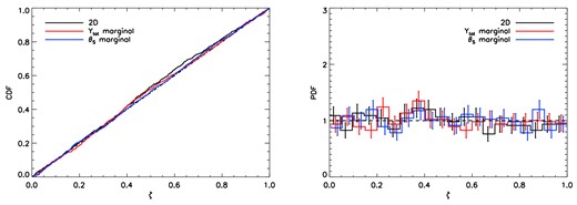
Left: the CDF of the standard uniform distribution (dot–dashed black line) and the empirical CDFs, for the full two-dimensional case (solid black line) and for the one-dimensional Ytot- and θs-marginals, respectively (red and blue solid lines), of the {ζk}-values obtained in the validation of posterior distributions |$\mathcal {P}_k(\theta _\mathrm{s},Y_\mathrm{tot})$| (k = 1, 2, …, Ncl) derived from Ncl = 918 simulated clusters injected into real Planck sky maps. The injected clusters have the same fixed ‘shape’ parameter values as assumed in the analysis, namely the ‘universal pressure profile’ (c500, γ, α, β) = (1.18, 0.31, 1.05, 5.49). Right: the PDF of the standard uniform distribution (dashed black line) and the empirical PDFs of the corresponding {ζk}-values (constructing by dividing them into 20 bins) for the full two-dimensional case (solid black line) and for the one-dimensional Ytot- and θs-marginals, respectively (red and blue solid lines); the error bars denote the Poissonian uncertainty.
The p-values for the null hypothesis, as obtained from our test for validating Bayesian inference analyses applied to the posterior distributions |$\mathcal {P}_k(\theta _\mathrm{s},Y_\mathrm{tot})$| (k = 1, 2, …, Ncl) derived from Ncl = 918 simulated clusters injected into real Planck sky maps. The second column gives the p-values for the case in which the injected clusters have the same fixed ‘shape’ parameter values as assumed in the analysis, namely the ‘universal pressure profile’ (c500, γ, α, β) = (1.16, 0.33, 1.06, 5.48). The third and fourth columns correspond, respectively, to when the injected clusters have γ = 0 and β = 4.13; see text for details.
| Correct profile | γ discrepancy | β discrepancy | |
|---|---|---|---|
| 2D | 0.09 | <10−8 | <10−8 |
| Ytot | 0.47 | 0.23 | <10−8 |
| θs | 0.93 | 0.06 | <10−8 |
| Correct profile | γ discrepancy | β discrepancy | |
|---|---|---|---|
| 2D | 0.09 | <10−8 | <10−8 |
| Ytot | 0.47 | 0.23 | <10−8 |
| θs | 0.93 | 0.06 | <10−8 |
For the purposes of interpretation, it is again useful to consider the corresponding PDFs, which are plotted in the right-hand panel of Fig. 10. These are again constructed by dividing the ζ-range [0, 1] into 20 bins of equal width, which provides the necessary resolution to constrain departures from uniformity in the wings of the distribution (ζ > 0.95). We mentioned in Section 2.1 that the K–S test is not equally sensitive to the entire interval [0, 1] and note here that one of its insensitivities is to discrepancies in the wings. Directly testing whether the PDF in ζ is consistent with the uniform distribution, particularly in at high ζ-values, thus represents a useful complement to the n-dimensional K–S test. With a samples size of Ncl = 918 clusters and assuming Poisson statistics, one has a precision of about 14 per cent on the PDF in each bin. We see from the figure that the binned PDFs are all consistent with a uniform distribution.
We therefore conclude that the constraints on cluster parameters derived from the Planck SZ likelihood are robust (at least to the sensitivity of our test) to real-world complications regarding foreground emission and beam shapes.
4.2.4 Mismodelling of the cluster pressure profile
Finally, we consider the robustness of our parameter inference to mismodelling the pressure profile of the clusters. To this end, we generate two set of simulations in which the injected clusters have different values of the GNFW shape parameters to those assumed in the analysis. In the first set, we inject clusters with a core slope γ = 0, which is characteristic of morphologically disturbed clusters (Arnaud et al. 2010; Sayers et al. 2013). In the second set, we assume β = 4.13 for the outer slope, which is the best-fitting value for the mean profile of a sample of 62 bright SZ clusters using a combination of Planck and X-ray data (Planck Collaboration V 2013).
These two sets of simulations are then analysed and resulting posterior distributions validated in the same way as discussed above. For each set, the empirical CDF of the resulting {ζk}-values, as derived from the Ytot-marginal, are shown in the left-hand panel of Fig. 11 and the p-values obtained from our test (both for the two-dimensional case and the marginals) are given in the third and fourth columns of Table 4, respectively. For a discrepancy in γ, one sees that the test applied to the marginal posteriors is insensitive to mismodelling the cluster profile, but that the test on the joint two-dimensional posteriors rejects the null hypothesis at extremely high significance. By contrast, for a discrepancy in β, the test applied to the two-dimensional posteriors and both marginals all clearly reject the null hypothesis.

As in Fig. 10, but showing only results derived from the Ytot-marginal, for the case in which the injected clusters have γ = 0 (red line) and β = 4.13 (blue line), respectively.
One may instead interpret the above results as indicating that the inference process produces Ytot- and θs-marginal posteriors (and parameter estimates derived therefrom) that are robust (at least to the sensitivity of the test) to assuming an incorrect value of γ in the analysis, but that their joint two-dimensional posterior is sensitive to this difference. By contrast, the joint distribution and both marginals are sensitive to assuming an incorrect value of β.
To assist in identifying the nature of this sensitivity, it is again useful to consider the binned, empirical PDFs of the {ζk}-values; these are plotted in the right-hand panel of Fig. 11 for the test applied to the Ytot-marginal. In keeping with the other results, one sees that the PDF is consistent with a uniform distribution in the case of a discrepancy in γ, but is clearly different when there is a discrepancy in β. Moreover, one sees that this difference is most apparent at large ζ-values. Indeed, the shape of the PDF is consistent with an underestimation by ∼30 per cent of the area of the 1σ contour of the posterior distribution, which would not be too serious in some applications. Further investigation shows, however, that the problem here is associated with the extent of the derived posterior, but a bias low in the peak location of around 10 per cent. This bias is subdominant to the statistical uncertainty for most clusters in the sample but is the dominant source of error for high signal-to-noise ratio clusters. Furthermore, as a coherent systematic across the whole sample, such an error could have damaging influence on derived information such as scaling relations or cosmological parameters.
5 CONCLUSIONS
In this paper we first present a practical extension of the K–S test to n-dimensions. The extension is based on a new variable ζ that provides a universal |$\mathbb {R}^n \rightarrow [0,1]$| mapping based on the probability content of the HPD region of the reference distribution under consideration. This mapping is universal in the sense that it is not distribution dependent. By exploiting this property one may perform many simultaneous tests, with different underlying distributions, and provide an ensemble goodness-of-fit assessment.
We then present a new statistical procedure for validating Bayesian posterior distributions of any shape or dimensionality. The power of the method lies in the capacity to test all of the assumptions in the inferential machinery. The approach goes beyond the testing of software implementation and allows robust testing of the assumptions inherent in the construction of the likelihood, the modelling of data and in the choice of priors. This approach enables the observables to inform our understanding of the importance the various components of the model given the data. It is, therefore, possible to tune the complexity of a model to reflect the information actually available in the posterior, improving the parsimony of the inference in keeping with Occam's Razor. Conversely, important hidden parameters or overly restrictive prior assumptions can be identified and treated properly.
In the application to SZ cluster parameter inference from Planck data, we demonstrate how the method can be applied to a large population where the posterior distributions vary. The information from a full cluster population can be combined to test the inference in the presence of varying stochastic and systematic uncertainties, as well as a varying signal component. For this application, we have found that the simplified Planck cluster likelihood is robust to real-world complications such as Galactic foreground contamination and realistic beams. The sensitivity of the inference to prior assumptions on the outer slope of the pressure profile has been identified, as has the insensitivity to assumptions on the pressure profile in the core regions of the cluster for the inference of the integrated Compton-Y parameter.
This approach could be of use in improving the pool of available SZ data from high-resolution microwave experiments, which to date have provided either non-Bayesian point estimates for cluster parameters or parameter proxies (Hasselfield et al. 2013; Reichardt et al. 2013), or unvalidated Bayesian posterior distributions (Planck & AMI Collaborations 2013). These experiments have different dependencies on cluster parameters given their different resolutions, parametrizations and observation frequencies. A fuller understanding of the nature of these dependencies and the sensitivity of the derived posteriors to assumptions of the cluster model will ensure the robustness of the results and maximize the wider scientific returns due to the complementarity of the data sets.
Beyond astronomy, the methodology we have introduced may be applied to Bayesian inference more generally, in any situation where higher levels of complexity and fidelity can be introduced into simulations than can be allowed for in a tractable analysis, or where there exists a pool of pre-existing real data with known outcomes.
This work was supported by the UK Space Agency under grant ST/K003674/1. This work was performed using the Darwin Supercomputer of the University of Cambridge High Performance Computing Service (http://www.hpc.cam.ac.uk/), provided by Dell Inc. using Strategic Research Infrastructure Funding from the Higher Education Funding Council for England and funding from the Science and Technology Facilities Council. The authors thank Mark Ashdown, Steven Gratton and Torsten Enßlin for useful discussions, and Hardip Sanghera and the Cambridge HPC Service for invaluable computing support. We also thank the referee, John Peacock, for numerous insightful comments that undoubtedly improved the paper.
An efficient implementation for evaluating QKS may be found in Press et al. (2007).
Another possibility is to divide the range of |$f(\boldsymbol {x})$| into NB bins with, in general, unequal widths |$\Delta _f^{(b)}$|, which are chosen such that each corresponding region |${\cal R}_b$| contains the same probability mass. This would ensure that each region contains a similar number of coloured data points, but could lead to regions within which the value of |$f(\boldsymbol {x})$| varies considerably (i.e. |$\Delta _f^{(b)}$| is large), and so data points will be far from uniformly distributed. We will investigate this alternative approach in future work.
The same criticism also applies to maximum aposteriori probability (MAP) estimators; in contrast, maximum likelihood (ML) estimators are reparametrization invariant.
REFERENCES
