


Abstract
PSR B0823+26, a 0.53-s radio pulsar, displays a host of emission phenomena over time-scales of seconds to (at least) hours, including nulling, subpulse drifting, and mode-changing. Studying pulsars like PSR B0823+26 provides further insight into the relationship between these various emission phenomena and what they might teach us about pulsar magnetospheres. Here we report on the LOFAR (Low-Frequency Array) discovery that PSR B0823+26 has a weak and sporadically emitting ‘quiet’ (Q) emission mode that is over 100 times weaker (on average) and has a nulling fraction forty-times greater than that of the more regularly-emitting ‘bright’ (B) mode. Previously, the pulsar has been undetected in the Q mode, and was assumed to be nulling continuously. PSR B0823+26 shows a further decrease in average flux just before the transition into the B mode, and perhaps truly turns off completely at these times. Furthermore, simultaneous observations taken with the LOFAR, Westerbork, Lovell, and Effelsberg telescopes between 110 MHz and 2.7 GHz demonstrate that the transition between the Q mode and B mode occurs within one single rotation of the neutron star, and that it is concurrent across the range of frequencies observed.
1 INTRODUCTION
The average pulse profile shapes of radio pulsars are remarkably stable when summed over at least a few hundred rotations. This reflects their clock-like rotational predictability (e.g. Liu et al. 2012) and enables their use as precision physical probes (e.g. Weisberg & Taylor 2005; Hobbs et al. 2010; Van Eck et al. 2011). None the less, pulsar emission variability has been recognized on almost all time-scales that are observationally accessible (e.g. Keane 2013): from nanosecond ‘shots’, expected to be the quanta of pulsar emission (Hankins et al. 2003), to multidecadal variations presumably due to evolution of the magnetic field (Lyne et al. 2013).
Indeed, there are a number of common emission phenomena which show that pulsar magnetospheres can be both stable and dynamic. For instance, drifting subpulses are a periodic drift of consecutive single pulses through the average pulse window, at a rate of tenths to a few times the spin period (Drake & Craft 1968; Weltevrede, Edwards & Stappers 2006a). Furthermore, hundreds of pulsars show nulling: a sudden cessation in emission between otherwise strong and steady pulses, spanning one to a few spin periods in most cases, but lasting upwards of several hours in some cases (e.g. Wang, Manchester & Johnston 2007). Extreme nulling events can last for days to years (such sources are sometimes termed ‘intermittent pulsars’ depending on the arbitrary length of time for which the pulsar is undetected). As with shorter nulls, the transition between the detected emission, ‘ON’, and the null state, ‘OFF’, occurs in less than 10 s, and perhaps within a single rotation (Kramer et al. 2006). For longer term nulling pulsars, the spin-down rate during the ‘ON’ state has been detected to be approximately 1.5–2.5 times larger than that during the ‘OFF’ state (Kramer et al. 2006; Camilo et al. 2012; Lorimer et al. 2012).
Mode-changing is a similarly abrupt switch in the pulsed emission between two (or more) discrete and well-defined pulse profile morphologies (Lyne 1971; Rankin, Wolszczan & Stinebring 1988) that are observed to occur over the same time-scales as pulse nulling (i.e. seconds to years; e.g. Wang, Manchester & Johnston 2007; Weltevrede, Johnston & Espinoza 2011; Brook et al. 2014). This is also occasionally identified in variable linear (Backer, Rankin & Campbell 1976) and circular polarization (Cordes, Rankin & Backer 1978). In some cases, pulse profile changes are also correlated with large changes in spin-down rates (0.3–13 per cent; Lyne et al. 2010).
The above emission phenomena are thought to be connected, and related to changes in the current flows in the pulsar magnetosphere (Lyne et al. 2010; van Leeuwen & Timokhin 2012; Li, Spitkovsky & Tchekhovskoy 2012b). For example, nulls can be regarded as a mode during which emission ceases or is not practically detectable. Most pulsars may exhibit these emission phenomena, but the effects of pulse-to-pulse variability are hard to identify in sources with low flux densities, because summing over many pulses is required to achieve sufficient signal-to-noise ratio (S/N). Also, it is possible that fewer pulsars are identified with longer characteristic time-scale phenomena, such as mode-changing and extreme nulling, because frequent observations over a longer timespan are necessary to enable this. The hope is that better understanding these emission characteristics may lead to a better understanding of the magnetospheric emission mechanism itself.
PSR B0823+26 is the focus of this work because it has been shown to exhibit a host of emission phenomena. This includes bursts of subpulses that drift slowly in longitude, towards both the leading and, more commonly, trailing edge of the main pulse (Weltevrede, Stappers & Edwards 2007). The nulling fraction (NF) has previously been estimated to be 7(2) per cent,1 and nulls occur clustered in groups more often than at random (Herfindal & Rankin 2009; Redman & Rankin 2009). Recently, Young et al. (2012) showed that PSR B0823+26 nulls over a broader range of time-scales (from minutes to at least five hours), and that the pulsar is detected only 70–90 per cent of the time when observed. They also found no detectable change in spin-down rate between emitting and long null states to a limit of less than 6 per cent fractional change. Long-term timing of the pulsar shows relatively high timing noise residuals of 89 ms (Hobbs et al. 2004), including changes in the sign of the spin frequency second derivative (Shabanova, Pugachev & Lapaev 2013). Thus, PSR B0823+26 is a good candidate for studying how the many facets of the pulsar emission mechanism are observed and related in one source. However, admittedly this may complicate matters for studying any one of these properties individually.
PSR B0823+26 was one of the first pulsars to be discovered (Craft, Lovelace & Sutton 1968), and is one of the brightest radio pulsars in the northern sky, with 73(13) mJy flux density at 400 MHz (Lorimer et al. 1995) and a distance of 0.32|$^{\rm {+(8)}}_{\rm {-(5)}}$| kpc (Verbiest et al. 2012). It has been detected from 40 MHz (Kuz'min, Losovskii & Lapaev 2007) up to 32 GHz (Löhmer et al. 2008), with little profile evolution (Bartel, Sieber & Wielebinski 1978). It is also one of ten slowly-spinning, rotation-powered pulsars with pulsations detected in X-rays (Becker et al. 2004). The interpulse in the pulse profile suggests that it is nearly an orthogonal rotator, which is also supported by polarization observations (Everett & Weisberg 2001).
To further investigate the emission phenomena displayed by PSR B0823+26, we conducted radio observations at low frequencies (<200 MHz) using the Low-Frequency Array (LOFAR), where brightness modulation due to scintillation is averaged out across the band. We also conducted simultaneous observations using the LOFAR, Westerbork, Lovell, and Effelsberg telescopes to record data from 110 MHz to 2.7 GHz.
The observations and data reduction are described in Section 2. In Section 3, we report on the data analysis and results of the observations. We show that the long-term nulls previously reported are in fact a very weak and sporadically emitting mode, similar to that identified in PSR B0826−34 (Esamdin et al. 2005). Hereafter we refer to this mode as the ‘quiet’ (Q) emission mode, and therefore the regular strong emission as ‘bright’ (B), analogous to other mode-changing pulsars.2 In Section 4, we discuss these and further results and present our conclusions.
2 OBSERVATIONS
LOFAR observations of PSR B0823+26 were obtained on 2011 November 13–14, 2012 February 9, and 2013 April 7 (see van Haarlem et al. 2013 for a description of LOFAR). Between 5 and 21 High-Band-Antenna (HBA) core stations were coherently combined using the LOFAR Blue Gene/P correlator/beam-former to form a tied-array beam (see Stappers et al. 2011 for a description of LOFAR's pulsar observing modes). For a summary of the specifications of the observations, see Table 1.
Starting at 23:18 ut on 2011 November 13, and ending at 08:12 ut on 2011 November 14, 26 three-minute observations were taken with a gap of 19 min between successive observations. Data were taken using the central six core stations (the ‘Superterp’), and were written as 32-bit complex values for the two orthogonal linear polarizations at a centre frequency of 143 MHz and bandwidth of 9.6 MHz. PSR B0823+26 switched to emitting in the B mode during the 13th observation. The pulsar was not detected during the other 25 similar observations in this campaign, even after all observations were summed together in time.
To further evaluate the moding behaviour at LOFAR frequencies, a longer, three-hour observation was taken on 2012 February 9 using five of the central HBA core stations. The linear polarizations were summed in quadrature and the signal intensities (Stokes I) were written out as 32-bit, 245.76-μs samples, at a centre frequency of 143 MHz with 47.6 MHz bandwidth.
To investigate the broad-band behaviour of PSR B0823+26, a further eight-hour observation on 2013 April 7 was conducted simultaneously using LOFAR and three telescopes observing at higher frequencies: the Westerbork Synthesis Radio Telescope (WSRT), the Lovell Telescope and the Effelsberg 100-m Telescope; see Table 1 for a summary. The LOFAR observation used 21 HBA core stations, where the linear polarizations were summed in quadrature, and the signal intensities (Stokes I) were written out as 32-bit 245.76-μs samples, at a centre frequency of 149 MHz with 78 MHz bandwidth. The WSRT observation was taken in tied-array mode using the PuMaII pulsar backend (Karuppusamy, Stappers & van Straten 2008). Baseband data were recorded for eight slightly overlapping 10-MHz bands, resulting in a total bandwidth of 71 MHz centred at 346 MHz. The Lovell Telescope observed the pulsar using the digital Reconfigurable Open Architecture Hardware (ROACH) backend. Dual polarizations were Nyquist sampled over a 400-MHz band centred at 1532 MHz and digitized at 8 bits. The Effelsberg 100-m Telescope observation was conducted using the PSRIX backend (ROACH-board system for online coherent dedispersion) that recorded data at a centre frequency of 2635 MHz with 80 MHz bandwidth.
The data from the LOFAR observations were converted to 8-bit samples offline. Data from all observations were coherently dedispersed, except the LOFAR observations on 2012 February 9 and 2013 April 7 that were incoherently dedispersed, and folded using the pulsar's rotational ephemeris (Hobbs et al. 2004) and the dspsr program (van Straten & Bailes 2011), to produce single-pulse integrations. Radio frequency interference (RFI) in the pulsar archive files was removed in affected frequency subbands and time subintegrations using both automated (paz) and interactive (pazi) programs from the PSRCHIVE3 library (Hotan, van Straten & Manchester 2004). The LOFAR polarization data were calibrated for parallactic angle and beam effects by applying a Jones matrix (see Noutsos et al. 2015 for further details). The linear polarization parameters in the LOFAR data from the 2011 November 14 observation were also corrected for Faraday rotation, see Section 3.1 for further details.
3 ANALYSIS AND RESULTS
Here we describe the analysis and results of the observations summarized in Table 1. PSR B0823+26 switched between emission modes at least once during each observing campaign. Initially, we focus on the time- and frequency-averaged properties at LOFAR frequencies, Section 3.1, and at a range of frequencies, Section 3.2. In Section 3.3, we focus on the single-pulse analysis of the data from the simultaneous observations.
Summary of observations. Columns 1–8 indicate the observing telescope, date, start time, integration time, centre frequency, bandwidth, individual channel width, and sampling time. Column 9 shows the duration of the B mode relative to the start time, where ‘+’ indicates that the pulsar remained in the B mode until at least the end of the observation. For the LOFAR observations on 2011 November 14, 2012 February 9, and 2013 April 7: the observation IDs are L34789, L45754, L119505, respectively; HBA[0,1] stations included in tied-array mode were CS00[2–7], CS00[2,3,4,6,7], and CS0[01–07,11,17,21,24,26,28,30,32,101,103,201,301,302,401], respectively. Due to increased observing bandwidth and number of stations used, the 2012 February 9 and 2013 April 7 LOFAR observations were two times and 10 times more sensitive than the original 2011 November 14 LOFAR observation, respectively.
| Telescope | Date | Start time | τint | Frequency | Bandwidth | Channel-width | τsamp | Time in B mode |
|---|---|---|---|---|---|---|---|---|
| (dd.mm.yyyy) | (ut) | (MHz) | (MHz) | (kHz) | (μs) | |||
| LOFAR | 14.11.2011 | 03:42 | 3.0 (min) | 143 | 10 | 12 | 81.9 | 1.69+ (min) |
| LOFAR | 09.02.2012 | 20:30 | 3.0 (h) | 143 | 48 | 12 | 245.8 | 2.71+ (h) |
| LOFAR | 07.04.2013 | 14:00 | 8.0 (h) | 149 | 78 | 12 | 245.8 | 3.07–3.11,5.09+ (h) |
| WSRT | 07.04.2013 | 14:00 | 8.0 (h) | 346 | 71 | 24 | 64.7 | 3.07–3.11,5.09+ (h) |
| Lovell | 07.04.2013 | 14:00 | 8.0 (h) | 1532 | 400 | 4000 | 518.2 | 3.07–3.11,5.09+ (h) |
| Effelsberg | 07.04.2013 | 14:43 | 7.3 (h) | 2635 | 80 | 195 | 259.1 | (3.07–3.11),5.09+ (h) |
3.1 Emission modes description
Fig. 1 shows an overview of the emission characteristics of PSR B0823+26 over the course of the three-minute LOFAR observation taken on 2011 November 14, during which the pulsar switched to B-mode emission. This is the only observation with recorded polarimetric information. Fig. 1, panel d, clearly shows the sudden increase in total flux density 1.69 min after the start of the observation. Panels e and f show that this is also the case for the polarized flux density. The B mode continues for at least 160 single pulses until the end of the observation. This is an inadequate number of pulses to obtain a stable average pulse profile, which is shown for comparison in Fig. 1, inset plots. The total duration of the B mode in this case is not known exactly. During all 12 preceding and 13 following three-minute observations no emission was detected, and we infer that PSR B0823+26 was either nulling and/or emitting in the Q mode. Assuming this was also the case during the 19-min gaps between the observations, the duration of the Q mode and/or nulling can be constrained to at least 4.4 h before and 4.75 h after the observation summarized in Fig. 1. This multihour duration is similar to the length of prolonged nulls also observed by Young et al. (2012). It is also possible that ‘flickers’ of emission on the order of minutes in duration, such as that shown in Fig. 1, could have occurred in between observations.
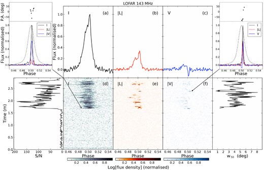
Overview plot of the LOFAR observation on 2011 November 14. Panels a,b, and c: time- and frequency-averaged pulse profiles for the B mode in total (Stokes I), linearly polarized (|L| = Stokes |$\sqrt{Q^{\rm 2}+U^{\rm 2}}$|), and circularly polarized (Stokes V) intensities, respectively. The average profile before the start of the B mode is not shown as it is indistinguishable from the noise in this short observation. Panels d,e, and f: the flux density of single pulses against pulse phase and integration time in total (increasing from white to black, see colour bars), linearly polarized (increasing from white to red), and absolute circularly polarized (increasing from white to blue) intensities, respectively. Lower left: S/N of total intensity single pulses against time. Lower right: full width at half-maximum, w50, against time for total intensity single pulses with S/N>7. Inset plots: normalized polarization profiles for two narrow and highly polarized single pulses indicated with arrows: initial B-mode pulse (left), and second pulse with similar characteristics at 2.4 min (right). Lower panels show the total (black), linearly polarized (red), and circularly polarized (blue) intensities. The stable average pulse profile in total intensity from the 2012 February 9 LOFAR observation is also shown (dashed line) for the same frequency and using the same timing ephemeris (from Pilia et al. 2015). Upper panels show the position angle of the linear polarization (P.A. = 0.5 tan−1(U/Q)).
Inspection of the single pulses from Fig. 1 shows that the transition between the Q and B modes is very rapid, occurring within one single rotational period. This is notable in the profiles of the single pulses and in the dramatic increase, by at least 60-times, in median S/N. We also note significant changes in the pulse width and morphology. Fig. 1, lower right, shows that the full width at half-maximum, w50, of the initial single pulses in the B mode are very narrow (1| $_{.}^{\circ}$|4), compared to the average pulse profile at the same frequency (7°, see Fig. 1, inset plots, and below). Subsequent B-mode pulses increase in width and drift towards earlier and later pulse phases until an equally narrow pulse (1| $_{.}^{\circ}$|1) occurs 80 pulses later at 2.40 min. This may be expected due to intrinsic variability e.g. subpulse drifting. Moreover, the narrow pulses are located towards the trailing edge of the average pulse profile, similar to what is observed from PSR B1133+16 (Kramer et al. 2003).
Further investigation of the polarization properties was also carried out. The Faraday rotation measure (RM) of the integrated pulse profile and the two narrow highly-polarized pulses was determined using RM-synthesis (Brentjens & de Bruyn 2005). The observed RM of the integrated B-mode pulse profile was determined to be 6.28(4) rad m−2. We find the RMs of the narrow single pulses to be consistent with this value. This RM value was used to correct the linear polarization Stokes parameters for Faraday rotation in order to maximize the linear polarization in the average pulse profile. The RM due to the interstellar medium (ISM) alone was determined to be 5.25(8) rad m−2, after correcting for ionospheric Faraday rotation (Sotomayor-Beltran et al. 2013). This is in good agreement with (within less than 2σ), and more precise than, the current ATNF pulsar catalogue4 value of 5.9(3) rad m−2 (Manchester 1974). The DM and corrected RM values can be used to determine the Galactic magnetic field direction and magnitude parallel to the line-of-sight towards PSR B0823+26 (e.g. Noutsos et al. 2008), which was calculated to be 0.332(6) μG. These results are discussed further in Section 4.5.
Variable pulse-to-pulse fractional polarization was also identified. The two narrow pulses previously identified show relatively high polarization (especially circular) fractions, see Fig. 1, inset plots. The initial B-mode pulse is 55(5) per cent right-hand circularly polarized, and the narrow pulse at 2.4 min is 56(5) per cent left-hand circularly polarized. The initial B-mode pulse and subsequent narrow pulse are 10(5) per cent and 38(5) per cent linearly polarized, respectively. The fractional circular polarization for these single pulses is therefore considerably larger than for the average pulse profile, which is 6(5) per cent circularly polarized and 15(5) per cent linearly polarized.
In order to further examine the moding behaviour, we observed PSR B0823+26 again for a continuous three-hour period using LOFAR on 2012 February 9. As shown in Fig. 2, lower panels, the pulsar switched from Q- to B-mode emission after 2.71 h. The lower panels of Fig. 2 clearly demonstrate that weak emission is detected from the start to 2.5 h into the observation, at approximately the same location in pulse phase as that of the main pulse during the B mode. This weak, but significant, Q-mode emission has not previously been detected; this mode was previously thought to be a long-term null. Between the weak Q mode at 2.55 h and the beginning of the B mode at 2.71 h, the flux density of the pulsar decreases even further and no emission is detected. PSR B0823+26 rapidly transitions to the B mode at 2.71 h, again within one single rotational period, and continues in this mode until the end of the observation. This is clear from the abrupt increase in S/N, see Fig. 2, lower right, and also in the pulse profile, see Fig. 2, upper panel. The ratio between the median S/N of single pulses in the B and Q modes is approximately 170.
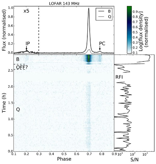
Overview plot of the LOFAR observation taken on 2012 February 9. Lower-left panel: flux density of the pulsar against pulse phase and integration time (logarithmic scaling, increasing from white through blue to green, see colour bar at the upper right). The modes of emission are identified: Q mode (0–2.55 h), B mode (2.71+ h), and, in the period of approximately 10 min in which the pulsar is not detected, tentatively ‘OFF?’ (2.55–2.71 h). These emission modes are delimited by the dashed lines. Subintegrations removed due to RFI are left blank, and the most affected time period is also labelled. Upper panel: time- and frequency-averaged total intensity pulse profiles separated by emission mode into Q (0–2.55 h, grey line) and B (2.71+ h, black line), normalized to the peak flux of the B-mode profile. The postcursor (PC) and interpulse (IP, 5× magnified) are also indicated. Lower-right panel: S/N of 42-s total intensity subintegrations against integration time.
Fig. 2, upper panel, illustrates the average pulse profiles of the Q and B modes. The B-mode pulse profile shows the known components from the literature, i.e. a narrow main pulse (MP), postcursor (PC), and interpulse (IP, separated by almost exactly half a rotation period from the MP) (see Backer, Boriakoff & Manchester 1973). The newly discovered Q-mode pulse profile is notably weaker. The location of the peak in flux density is also skewed towards slightly later pulse phases compared to the B-mode MP (+2(1)°, 2.9 ms). Table 2 includes a summary of the relative intensity, width and locations of the B and Q-mode pulse profile components. Details of how these were calculated are included in Section 3.2.
Summary of the pulse profile components from the LOFAR observation on 2012 November 9 (LOFAR1) and the simultaneous multifrequency observations on 2013 April 7. Columns 1 and 2 indicate the telescope and central frequency used. w50 of the B-mode MP, PC, and IP, and the Q-mode pulse are shown in columns 3, 7, 11, and 14, respectively. w10 of the B-mode MP and PC are summarized in columns 4, and 8, respectively. The peak flux location of the B-mode PC and IP, and the Q-mode pulse, with respect to that of the B-mode MP (where ‘+’ indicates later pulse phases) are shown in columns 5, 9, and 12, respectively. The relative amplitude of the peak flux of the B-mode PC and IP, and Q-mode pulse, with respect to the MP (corrected for different integration times using Table 1) are summarized in columns 6, 10, and 13, respectively. The bottom row shows the frequency dependence of each of the profile features as the exponent of a power law, η.
| B-mode MP | B-mode PC | B-mode IP | Q-mode | ||||||||||
|---|---|---|---|---|---|---|---|---|---|---|---|---|---|
| Telescope | Frequency | w50 | w10 | location | amplitude | w50 | w10 | location | amplitude | w50 | location | amplitude | w50 |
| (Name) | (MHz) | (°) | (°) | (°) | (per cent) | (°) | (°) | (°) | (per cent) | (°) | (°) | (per cent) | (°) |
| LOFAR1 | 143 | 6.68(5) | 14.06(8) | +31.5(1) | 3.76(5) | 9.8(3) | 17.9(5) | −178.5(7) | 0.90(5) | 20.5(6) | +2(1) | 0.89(5) | 9.4(2) |
| LOFAR | 149 | 6.73(3) | 13.36(8) | +31.5(1) | 3.19(5) | 9.6(2) | 17.4(2) | −179.3(2) | 0.75(5) | 16.2(5) | +1.9(2) | 0.62(5) | 9.6(4) |
| WSRT | 346 | 4.29(3) | 9.14(8) | +31.7(1) | 2.09(5) | 9.4(2) | 17.2(3) | −180.0(3) | 0.30(5) | 15.2(2) | +1.8(2) | 0.47(3) | 8.7(5) |
| Lovell | 1532 | 3.12(3) | 6.33(8) | +36.0(2) | 0.69(4) | 8.3(2) | 15.2(2) | −181(1) | 0.23(6) | 12.3(8) | +1.3(5) | 0.39(9) | 3.7(3) |
| Effelsberg | 2635 | 2.89(7) | 5.97(9) | +36.1(1) | 0.51(3) | 7.2(3) | 13.2(3) | −182(1) | 0.12(3) | 11(1) | +0.9(6) | 0.7(3) | 1.8(4) |
| All | η | −0.33(4) | −0.30(4) | +0.050(9) | −0.66(6) | −0.08(2) | −0.08(2) | +0.005(1) | −0.63(2) | −0.19(6) | −0.16(4) | −0.3(2) | −0.37(9) |
3.2 Multifrequency analysis
In light of previous studies of other pulsars (e.g. Hermsen et al. 2013), mode-switching is expected to occur over a broad-range of wavelengths, even up to X-rays. To investigate whether this is the case for PSR B0823+26, we observed the pulsar using four telescopes (LOFAR, WSRT, Lovell, Effelsberg) at a range of centre frequencies (149, 345, 1532, 2635 MHz) simultaneously. The overview of these eight-hour observations, Fig. 3, shows that both Q and B modes were detected again, and that the behaviour of PSR B0823+26 is very similar across the range of frequencies.
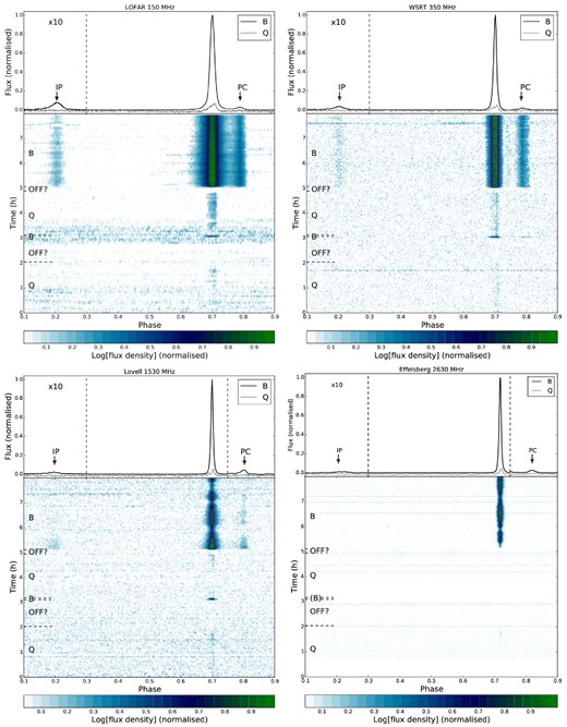
Overview of the multifrequency simultaneous observations taken on 2013 April 7, using: LOFAR (upper left), WSRT (upper right), Lovell (lower left), and Effelsberg 100-m (lower right). Upper panels: time- and frequency-averaged total intensity pulse profiles separated into the Q mode (0–3.07 h, 3.11–5.09 h; 10× magnified; grey lines) and the B mode (3.07–3.11 h, 5.09+ h, black lines), normalized to the peak flux of the B-mode profile. There also appear to be periods in which the pulsar is not detected (‘OFF?’; ∼2–3.07 h, 4.8–5.09 h). The PC (10× magnified in the lower plots) and IP (10× magnified) are also indicated. Lower panels: flux density of the pulsar against pulse phase and integration time (increasing from white through blue to green, see colour bars). Subintegrations removed due to RFI are shown as white. The modes of emission identified (Q, B, and, tentatively, ‘OFF?’) are also labelled, and these are delimited by the dashed lines. The off-pulse noise level in the LOFAR observation shows an increase around the transition from Q- to B- to Q-mode emission around 3 h because there was a period of increased RFI around this time, and more conservative RFI flagging was done to conserve as much data around this period as possible. Modulation of the B-mode brightness due to scintillation is also visible in the higher frequency Lovell and Effelsberg data.
The lower panels in Fig. 3 show that from the beginning of the observations until approximately 2 h, the weak Q-mode emission is visible at all four frequencies. Between ∼2 and 3.07 h the Q mode becomes even more weak and is practically undetectable. After this, the pulsar abruptly ‘flickers’ into B mode emission for approximately 160 pulses. The pulsar transitions back into the weakly-emitting Q mode between 3.11 and 4.8 h, which is most clearly detected at the two lower frequencies, but also towards the end of this period at the two higher frequencies. The flux in the Q mode once again decreases even further and becomes practically undetectable between 4.8 and 5.09 h, just before the pulsar transitions again into the B mode for the remainder of the observation. This is also demonstrated in terms of S/N against observing time in Fig. 4.
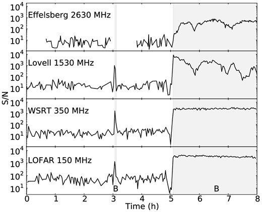
S/N of total intensity pulses versus integration time from the multifrequency simultaneous observations of PSR B0823+26. Upper to lower panels: Effelsberg 100-m at 2635 MHz using 80-s subintegrations; Lovell at 1532 MHz using 140-s subintegrations; WSRT at 345 MHz using 140-s subintegrations; LOFAR at 149 MHz using 110-s integrations. Discontinuation of lines indicates flagged subintegrations due to RFI. The periods of B-mode emission are indicated by the shaded grey backgrounds and labelled ‘B’.
Fig. 3, upper panels, illustrate the B-mode profiles and the previously unknown and much weaker Q-mode pulse profiles between 110 MHz and 2.7 GHz. The B-mode MP, PC, and IP are visible at all frequencies and, as expected from the literature, there is little profile evolution across the observed frequency range. Again, the Q mode is much weaker compared to the MP of the B mode, and the average peak flux occurs towards slightly later pulse phases (>+1°, depending on frequency).
On all occasions where the emission switches from the Q to B mode, the transition occurs within one single rotational period at all frequencies, identified by the notable increase (70×) in S/N of single pulses and change in pulse profile morphology. Fig. 3, lower panels, also show that the mode switch from Q to B at 5.1 h occurs simultaneously for all pulse profile components, i.e. the MP, PC, and IP, at all frequencies.
To determine whether the mode-switch occurs coincidently across all frequencies observed, the MJD of the initial B-mode single-pulse after the mode change was determined for each frequency. The expected time delays of equivalent pulses due to dispersion in the cold plasma of the ISM between the centre frequencies used at Effelsberg, Lovell, and WSRT and the centre frequency used at LOFAR are 3.63, 3.61, and 2.97 s, respectively. Taking this into account, we find that the mode-switch is coincident at the frequencies observed to within 0.01 s.
On the single occasion where we observe the pulsar switch from the B to Q mode, it is more difficult to pinpoint the transition because the flux density of single pulses decreases gradually over a few rotational periods, similar to the behaviour during the 2011 November 14 observation shown in Fig. 1, panel d, rather than showing an abrupt change in S/N. For the three lower frequencies, B-mode emission was detected over a 160 single-pulse time-scale during the B-mode ‘flicker’ at 3.1 h. Since the transition from the Q to B mode was determined to be simultaneous across the observed band, it is probable that this is also the case for the B-to-Q-mode change.
Fig. 4 shows the S/N against time for the simultaneous observations. This clearly demonstrates the simultaneous wide-band transitions between emission modes, especially the decrease in flux density in the Q mode just before the rapid transition to the B mode at 5.1 h. Here we again see that the B and Q mode differ in median flux density by over two orders-of-magnitude.
Fig. 4 illustrates fluctuations in pulse total intensity due to scintillation, which are much more evident in the prolonged B-mode emission at the two higher observing frequencies. This is because the scintillation bandwidth becomes comparable to the observing bandwidth at the higher frequencies. The DM of PSR B0823+26, measured using the LOFAR observation on 2013 April 7 using the PSRCHIVE pdmp program (Hotan et al. 2004), was found to be 19.475(3) pc cm−3. This amount of dispersion contributes to PSR B0823+26 falling into the strong diffractive scintillation regime when observed below approximately 5 GHz (Daszuta et al. 2013). At lower frequencies the scintillation bandwidth is much smaller, causing its effects to be averaged out more effectively across the band.
The B- and Q-mode multifrequency average pulse profiles obtained from the 2012 November 9 and 2013 April 7 observations, see Figs 2 and 3, were used to compare the behaviour of the pulse profile components with frequency. The profile components were fitted with Gaussian functions using the Levenberg–Marquardt algorithm (Levenberg 1944) to provide the normalized peak amplitude, peak location, w50, and full width at tenth of maximum, w10, values, and their respective errors. Table 2 provides the summary of these characteristics for the pulse profile components at multiple frequencies for B- and Q-mode emission. Peak amplitude is measured in percentage relative to the B-mode MP.
After quantifying characteristics of the profile features at each frequency listed in Table 2, the trend with respect to frequency was explored. Assuming that each feature, x, follows a power law with respect to frequency, x ∝ νη, a weighted best fit was performed to determine the appropriate value for the exponent, η. The resulting values and errors for the exponents are shown in the bottom row of Table 2.
We find that the width of all pulse profile components decrease with increasing frequency in both emission modes, although this trend is most notable for the Q-mode pulse. This is consistent with previous results for the B-mode pulse profile (e.g. Kramer 1994), and also with radius-to-frequency mapping (RFM; e.g. Gil et al. 2002). The largest intrachannel DM smearing at the lowest LOFAR frequency accounts for 0| $_{.}^{\circ}$|3 in pulse longitude, which does not affect the conclusions obtained from the low-frequency pulse profile. The B-mode PC and IP move further from the MP and decrease in amplitude relative to the MP with increasing frequency. The positions of the PC and IP and their frequency dependence are in agreement with previous results (Hankins & Fowler 1986). This is further discussed below in Section 4. Table 2 shows that the amplitude of the PC has the strongest frequency dependence and the location of the IP is the least dependent on frequency.
The relative pulse amplitude of the Q-mode profile is approximately equal to the amplitude of the B-mode IP, and also decreases with increasing frequency. The peak amplitude of the Q mode is located towards later pulse phases compared to the B-mode MP at the same frequencies, and seems to arrive progressively earlier in pulse phase towards higher frequencies. Furthermore, Table 2 shows that both B- and Q-mode pulse profiles show no significant change over one year between the LOFAR observations from 2012 February 9 and 2013 April 7.
To further investigate the relative properties of the B and Q modes at low-frequency, the spectrum in each mode was calculated using the eight-hour LOFAR observation. The flux density, S, as a function of frequency was obtained using the radiometer equation, including an empirically-derived and tested formula for the effective area of the LOFAR stations, and correction for the primary beam using the theoretically-derived and tested beam model, described in Hassall, et al. (in preparation), and references therein. The B-mode and Q-mode data were divided into 5 and 3 subbands, respectively, deemed to be appropriate to optimise the respective S/N. A line of best fit was calculated assuming a single power law across the bandwidth of the observation, S ∝ να, and the error was determined considering the flux density errors only. Fig. 5 shows the resulting spectra in the two emission modes.
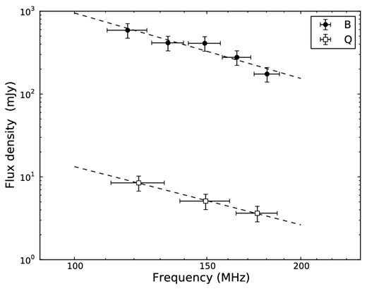
Low-frequency spectra of PSR B0823+26, separated into B- (filled circles) and Q-mode emission (open squares), obtained from the LOFAR observation taken on 2013 April 7. Frequency-axis error bars show the bandwidth used to calculate each point. The dashed lines show the best power-law fit to the data.
The difference in flux density between the B and Q modes is striking, see Fig. 5. In fact, the average flux density in the B mode, 370 mJy at 149 MHz, is almost two orders-of-magnitude greater than that of the Q mode, 5 mJy. This is probably a factor in the previous non-detection of this weak Q mode.
The exponent, α, obtained from the continuous power-law best fits, weighted by the uncertainties, for the B and Q-modes are −2.6(5) and −2.3(1), respectively. Therefore, there is no significant difference in the power-law index of the spectra between emission modes. This is further discussed in Section 4. The relatively steep spectral index and strong scintillation are also possible factors in the previous non-detection of the weak Q-mode emission at higher frequencies. The increased bandwidth used for the observation using the Lovell Telescope on 2013 April 7 in this work (400 MHz) also provided almost a factor of 2 better sensitivity in comparison to the observations in Young et al. (2012).
3.3 Single-pulse analysis
Potentially interesting emission features were investigated and compared for the B and Q modes by analysing single pulses from the eight-hour simultaneous observations. This was conducted using a software package provided by Weltevrede (private communication) to construct centred, gated, de-baselined, and further RFI-excised single-pulse archives (e.g. Weltevrede et al. 2006b). This enabled us to extract information regarding nulling, subpulse drifting, and pulse energy distributions (PEDs).
3.3.1 Pulse energy distributions
Longitude-resolved PEDs were calculated for each pulse profile component of the B and Q modes by integrating over a selected pulse longitude bin range, see Fig. 6. Pulse longitude ranges corresponding to w10 were selected to optimise S/N. These are indicated underneath the average pulse profiles in Fig. 6, upper panels. The longitude range of the off-pulse (OP) region shown in Fig. 6 was selected to correspond to the range selected for the Q-mode pulse, and to be located mid-way between the B-mode MP and IP.
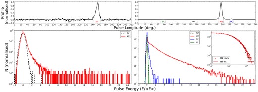
Upper panels: normalized average pulse profiles (black line) for the Q mode (left) and B mode (right), showing longitude ranges included in the pulse-energy analysis (delimited by the black dotted lines). Lower panels: normalized longitude-resolved PEDs for the Q- (left) and B-mode emission (right), using the LOFAR observation taken on 2013 April 7. The MP, PC, IP, and off-pulse (OP) distributions are shown (red, blue, green, and black dotted lines, respectively). Inset panel: B-mode MP PED data (red points) and best lognormal fit to the data (red line), plotted on logarithmic axes.
Fig. 6, upper panels, shows the normalized flux-density profiles of the B and Q modes. Note the difference in the OP noise level. The lower panels in Fig. 6 illustrate the normalized PED with respect to the average pulse energy, 〈E〉, shown separately for the Q (left) and B modes (right). The B-mode MP and PC PEDs are clearly distinct from that of the OP region and resemble lognormal probability density distributions, see the inset panel. Using a method similar to that in Weltevrede et al. (2006b), the best lognormal fit to the PED for the MP for pulse energies 1.5–20 times greater than the average yields a standard deviation of 0.77(15). The IP PED is comparable to that found for the OP region because of its relatively weak single-pulse flux.
Q-mode emission shows a distinctly different PED, which falls off much more rapidly at low energies and resembles a power-law distribution. The Q-mode PED is less distinguishable from that of the OP region at lower pulse energies due to the much weaker emission, but shows a tail of less frequent higher-energy pulses. The best power-law fit to the PED for pulse energies one to eight times greater than the average gives an exponent of −3.2(2).
To investigate how the energy of the pulses affects the average pulse profile, we constructed integrated PEDs from the longitude-resolved PEDs, shown in Fig. 6, to obtain the average pulse profile for a number of pulse energy ranges. We find that the most energetic B-mode single pulse profiles show PCs located towards lagging pulse phases. Moreover, these pulses are approximately eight times brighter compared to the average pulse profile. Despite this, the average pulse profile shows remarkably little pulse profile evolution with increasing pulse energy, similar to that observed in PSR B1133+16 (Kramer et al. 2003). In addition, single pulses with the highest flux in the Q mode have smaller w50 values than the average pulse profile. There is also a more notable contrast in pulse profile evolution with energy in the Q mode. That is, pulses with energies greater than twice the average possess profiles akin to a skewed Gaussian, similar to that in Fig. 6, top left. Pulses with energies less than twice the average have profiles that are weak (discernible from the baseline at approximately 3σ), irregular, and somewhat top-hat-like in shape, for examples see Fig. 7, left. Hence, the pulse profiles in the Q mode seem to show much greater variability with energy compared to those in the B mode.
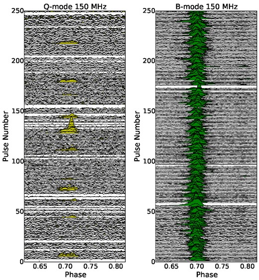
Representative examples of single-pulse profiles from the LOFAR observation on 2013 April 7, arbitrarily normalized. Left: sporadic and weak emission during the Q mode, right: B-mode regular emission for comparison. Single pulses rejected due to RFI are not shown.
3.3.2 Nulling
The integrated PEDs were used for complimentary analysis of the NF. We estimated the NFs by subtracting the OP pulse-energy samples from the on-pulse PEDs, as described in Wang et al. (2007). The analysis was undertaken separately for the Q mode, the 160-pulse B-mode ‘flicker’, and the prolonged B mode from the 2013 April 7 LOFAR observation, summarized in Fig. 3.
PSR B0823+26 displays nulling in both emission modes. More specifically, the NF for the prolonged B-mode was determined to be 1.8(5) per cent. This is lower than, but still within 2.2σ of, previous estimates (Herfindal & Rankin 2009). The NF for the B-mode ‘flicker’ was found to be 15(1) per cent – almost 10 times larger than that during the prolonged B-mode emission.
Further inspection of the single pulses during this short-lived period of B-mode emission also indicates that the NF increases towards the transition back to the Q mode. Inspection of simultaneous pulses from the 346 MHz and 1.5 GHz data also indicate that the nulls occur simultaneously at all frequencies, which is consistent with mode-switching, and is observed in several other cases (e.g. Biggs 1992; Hermsen et al. 2013). The NF throughout both occurrences of the Q mode during the observation was determined to be 80(9) per cent. This indicates that there are over 40 times more nulls during the Q-mode than during B-mode emission. However, we note that the apparent nulls (in both B- and Q-mode emission) may be yet another weaker emission state that is currently undetectable.
Fig. 7, left, demonstrates the nature of the Q-mode emission through a 250-single-pulse extract from 4.6 h into the observation. A pulse extract from the B-mode emission is also shown in Fig. 7, right, for comparative purposes. The weak Q-mode emission consists of sporadic, mainly low-intensity bursts which occur in groups of approximately one to five pulses with no immediately identifiable periodicity. Therefore, PSR B0823+26 seems to display similar behaviour to the weak-mode emission identified in PSR B0826–34 (Esamdin et al. 2005), also somewhat resembling emission from rotating radio transients (RRATs; McLaughlin et al. 2006). This is also further discussed in Section 4.
3.3.3 Subpulse modulation features
The subpulse modulation properties of the prolonged B mode at low frequency were investigated using the LOFAR observation on 2013 April 7, and the method described in Weltevrede et al. (2006a). The aim was to compare the modulation patterns exhibited by the different modes (e.g. van Leeuwen & Timokhin 2012). Pulse stacks, for example see Fig. 7, were used to obtain the Longitude Resolved Fluctuation Spectrum (LRFS; Backer 1970) and hence the vertical separation between drift bands, P3, measured in pulse periods, P0. The LRFS obtained from the B-mode emission, Fig. 8, right, shows two drift features that are broader than 0.05 cycles per period (CPP). One feature is located at the alias border P0/P3 = 0, and the other feature relates to P3 = 5.26(5)P0. Since P3 is generally independent of observing frequency, this is in excellent agreement with the value of 5.3(1)P0 previously determined at 92 cm (Weltevrede et al. 2007).
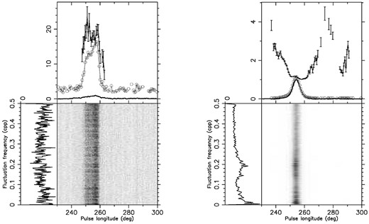
Pulse variability analysis products from the LOFAR observation on 2013 April 7, for the Q mode (left) and the B mode (right). Upper panels: the normalized integrated pulse profile (solid line), the longitude-resolved standard deviation (open circles), and the longitude-resolved modulation index (dimensionless quantity shown as the solid line with error bars). Lower panels: the LRFS is shown, with its horizontal integration to the left.
We also constructed Two-Dimensional Fluctuation Spectra (2DFS; Edwards & Stappers 2002) to determine the horizontal separation between the drift bands, P2, measured in pulse longitude. For the B-mode emission, we find that although the feature in the 2DFS peaks at zero CPP, the wings are asymmetric, indicating that drifting subpulses travel towards later pulse phases more often. Calculating the centroid of the asymmetric wings at 20 per cent of the maximum allowed us to extract the value of P2 = +90(20)°. This is in good agreement with the value obtained at 92 cm, +70°|$^{+10}_{-12}$| (Weltevrede et al. 2007). Unlike P3, P2 is found to vary with observing frequency (Edwards & Stappers 2003). Since P2 = +55°|$^{+40}_{-7}$| at 21 cm (Weltevrede et al. 2006a), the value determined here also seems to be in agreement with the general trend that P2 decreases with increasing observing frequency for PSR B0823+26.
The same subpulse modulation analysis was also conducted for the prolonged Q-mode emission from the 2013 April 7 LOFAR observation. No significant feature was detected in either the LRFS, Fig. 8, left, or 2DFS, indicating that there is variability on all fluctuation frequencies. This may be attributed to the greater NF and very weak single pulses. However, PSR B0943+10, which shares many emission characteristics with PSR B0823+26, also shows subpulse drifting during the B mode and not in the Q mode, which is also comparatively ‘disordered’ (Backus, Mitra & Rankin 2011).
The longitude-resolved modulation index, a measure of the factor by which the intensity varies from pulse to pulse, was derived from the LRFS (Weltevrede et al. 2006a), see Fig 8, upper panels. The median modulation index of the B-mode MP was found to be 1.4(5). The median modulation index of the PC component was found to be slightly larger, 1.6(9). The B-mode MP and PC components show similar longitude-resolved modulation characteristics, although the PC shows slightly more variability than the MP. The median modulation index of the Q-mode pulse was found to be over 10 times larger than the B mode MP, 17(5), and shows somewhat different longitude-resolved modulation compared to the B mode, see Fig 8, upper panels.
The pulse profile stability during the B mode was investigated using the 2013 April 7 simultaneous LOFAR and WSRT data. The Pearson product-moment correlation coefficient, ρ, was calculated between an analytic profile of PSR B0823+26 and the pulse profile integrated from an increasing number of effective single pulse numbers, Nefc, as described in Liu et al. (2012). We find that towards higher effective pulse numbers (>200–500) the LOFAR and WSRT data follow the expected trend, i.e. 1−ρ ∝ |$N_{\rm {efc}}^{\rm {-1}}$| (Liu et al. 2011). However, there are some notable deviations from this trend, which tend to coincide with narrow, bright pulses. This suggests that over many pulse periods the pulse profile is stable, but over short periods the emission shows intrinsic pulse-to-pulse shape variations. This is not unexpected due to previous results that show the array of emission phenomena exhibited by PSR B0823+26.
4 DISCUSSION AND CONCLUSIONS
In this work, we have confirmed that PSR B0823+26 shows a host of emission characteristics over a wide range of time-scales. The most surprising finding from the work presented here is that the long-term nulls, recently found by Young et al. (2012), are in fact a very weak and sporadically emitting mode, which we refer to as the Q mode. We find that this mode is over 100 times weaker than the B mode. We also find evidence for a further decrease in flux just before the switch to the B mode, see Figs 2 and 3. It is possible that this could be a third emission mode, whereby the flux density of emission decreases even further or emission completely ceases. It would also be quite interesting if this weakest (possibly completely off) mode is found to always occur before the start of the B mode – as it has in the three instances we have observed.
Considering the many studies which have been conducted on PSR B0823+26, it is surprising that the long-term nulling was only recently discovered (Young et al. 2012). It may be that the emission from PSR B0823+26 has changed over a multiyear time-scale, such that mode changing is more frequent or longer in duration than in previous years, though that remains to be shown. If so, this may be due to a multidecadal change in emission, perhaps related to that observed in the Crab pulsar due to magnetic field evolution (Lyne et al. 2013).
4.1 Magnetospheric switches
Upon investigation of the newly-discovered Q-mode pulse profile at frequencies between 110 MHz and 2.7 GHz, we find the pulse profile comprises a single component located within the regular B-mode MP envelope, but with a peak located towards slightly later pulse longitude, and a lower flux density by approximately two orders of magnitude. The PC and IP that are present during the B mode are not detected during the Q mode. A converse example of a pulsar that exhibits mode-changing, PSR B0943+10, has a precursor in the Q mode and not in the B mode at 320 MHz (Hermsen et al. 2013).
During the Q mode, the emission is weak and sporadic, with a very high NF and modulation index. This behaviour seems similar to the Q mode identified in PSR B0834–26 (Esamdin et al. 2005). It also seems reminiscent of RRAT-like emission that may imply a common, or at least related, emission mechanism. This has previously been proposed from both theoretical (e.g. Jones 2013) and observational perspectives (e.g. Burke-Spolaor & Bailes 2010; Keane et al. 2011). The detection of the weakly-emitting Q mode from PSR B0823+26 could mean that other pulsars currently identified as extreme-nullers may also show similar weak emission if higher-sensitivity observations can be done (Esamdin et al. 2005; Wang et al. 2007; Young et al. 2014).
During the simultaneous observation on 2013 April 7, the initial ‘OFF?’ period lasted approximately 0.87 h, and preceded the short-duration 160 single-pulse B-mode ‘flicker’. Later in the same observation, and also in the observation on 2012 February 9, the ‘OFF?’ period was much shorter in duration, and the subsequent B-mode emission was much longer in duration. This further decrease in radio emission, which tentatively may be considered as a further separate emission mode, could be caused by a change in the particle density within the magnetosphere that soon after causes the switch to the B mode. We also speculate that the duration of the undetected emission towards the end of the Q mode, just before the mode-switch to the B mode, may be inversely correlated with the length of time the pulsar emits in the subsequent B mode. We stress that this is speculative due to the limited sample, and more work will be done in future to investigate this by using longer and more frequent low-frequency observations.
Single-pulse analysis allowed us to determine that the transition from the Q mode to the B mode occurs within one rotational period, and that it is broad-band over the radio frequencies observed, similar to other mode changing pulsars (e.g. PSR B0943+10; Hermsen et al. 2013; Bilous et al. 2014), and nulling pulsars (e.g. PSR B0809+74; Bartel et al. 1981). Although, considering the tentative ‘OFF?’ mode just before the switch to B-mode emission mentioned previously, the underlying mode change mechanism may be more complex than is evident from the single-pulse data. Within the theoretical framework of force-free magnetospheres, it has been shown that multiple stable solutions with different structures are possible, e.g. with different sizes of closed field line region (Contopoulos 2005; Timokhin 2010). Therefore, the B and Q modes could be caused by two stable magnetospheric states with different magnetospheric structures, affecting the current of relativistic particles, and therefore the broad-band radio emission mechanism. However, the mechanism that generates the wide range of observed time-scales (e.g. each emission state lasting many hours and mode-switches occurring within one rotational period) is still elusive.
4.2 Considering spin-down
PSR B0823+26 shows no detectable change in spin-down rate between modes (Young et al. 2012), similar to other pulsars which exhibit mode-changing on similar time-scales, e.g. PSRs B0834–26 and B0943+10, whilst other extreme-nulling pulsars identified as ‘intermittent’ often do (Kramer et al. 2006; Camilo et al. 2012; Lorimer et al. 2012). In part, this is because it is difficult to detect small changes in spin-down if transitions occur more frequently than for the more extreme nulling pulsars (Young et al. 2012). This may also be due to the electromagnetic spin-down torque exerted on the neutron star, proportional to sin2θ + (1 − κ)cos2θ (Contopoulos & Spitkovsky 2006), where θ is the alignment angle between the spin axis and magnetic moment, and κ the ratio between the angular velocity of the pulsar and the angular velocity at the death line. Namely, if there is some small change in θ between emission modes, then the change in spin-down torque is less severe in cases of nearly orthogonal rotators (e.g. PSR B0823+26, Everett & Weisberg 2001). This is less certain in cases of nearly aligned rotators (e.g. PSR B0943+10; Deshpande & Rankin 2001) (Li, Spitkovsky & Tchekhovskoy 2012a).
4.3 Emission characteristics
Although we find that the spectral indices of the B and Q modes are consistent, within errors, the broad-band spectrum of PSR B0823+26 shown in Hassall et al. (in preparation) indicates a possible spectral turn-over at 127(25) MHz. Future observations using the LOFAR Low Band Antennas (30–90 MHz) would be ideal for further investigating the spectral properties of PSR B0823+26 in both emission modes (if the Q mode is detectable), including providing constraints on the presence of a spectral turn-over, and hence supplying more clues about the origin of the difference between emission modes.
PSR B0823+26 also shows certain emission characteristics which are reminiscent of several other pulsars. The PCs associated with the highest energy single pulses that are eight times brighter than average are reminiscent of the Vela pulsar's (PSR B0833−45) ‘bump’ component after the MP, where ‘giant micro-pulses’ with flux densities exceeding 10 times that of the mean were observed (Kramer, Johnston & van Straten 2002). For comparison to the highly polarized single pulses detected in the 2011 November 14 LOFAR observation, PSR B0656+14, which may be a nearby RRAT, also shows strong highly-polarized single pulses limited to the leading and central regions of the average pulse profile (Weltevrede et al. 2006b). Moreover, narrow pulses observed after the transition to the B mode occur towards the trailing edge of the average pulse profile, similar to that observed in PSR B1133+16 (Kramer et al. 2003). The presence of an IP located close to 180° pulse longitude from the MP, a highly linearly polarized PC (Weisberg et al. 1999; Noutsos et al. 2015) in the pulse profile, and B- and Q-mode emission is also reminiscent of PSR B1822−09 (Backus, Mitra & Rankin 2010; Latham, Mitra & Rankin 2012).
Polarization observations have allowed the MP to be classified as a core component and the IP to be classified as a possible core component of the opposite magnetic pole (Weisberg et al. 1999, and references therein). The PC's high linear polarization fraction could originate from induced scattering of the MP emission into the background by the particles of the ultrarelativistic highly magnetised plasma (Petrova 2008). This could also explain the trend in the PC location growing more distant with increasing frequency, which is contradictory to the behaviour expected from RFM (e.g. Mitra & Rankin 2002) and has led to reluctance in its classification as a conal component (Weisberg et al. 1999). We note that the decrease in the pulse profile component widths with increasing frequency is consistent with the RFM model (e.g. Gil et al. 2002), although this may also be caused by other mechanisms (e.g. birefringence, McKinnon 1997).
It seems that the emission behaviour observed from PSR B0823+26 is very diverse, and may prove one of the most difficult pulsars to model in terms of accounting for the host of emission characteristics that arise over many different time-scales. However, observations of PSR B0823+26 may also help in efforts to unify the diverse phenomenology of pulsar emission and provide vital data in terms of studies of the elusive pulsar emission mechanism.
4.4 Pulsar population implication
In the period–period-derivative (P–|$\dot{P}$|) diagram for non-recycled pulsars from the ATNF pulsar catalogue (Manchester et al. 2005), PSR B0823+26 is located near the centre of the distribution, and therefore appears to be a very regular pulsar in this parameter space. Other pulsars which have been identified to display at least one of the numerous emission characteristics investigated here are located throughout most of the parameter space, apart from the area occupied by very young pulsars. Therefore, there is no obvious correlation with surface magnetic field strength or characteristic age (e.g. Weltevrede et al. 2007). Most pulsars may exhibit these emission phenomena, but the effects of pulse-to-pulse variability are diminished due to summing over many pulses, which is required to achieve sufficient S/N in the case of sources with low flux densities.
To date, only a handful out of the ∼2300 known pulsars are identified as intermittent or extreme nullers. This is because this requires frequent observations over several months/years to identify this long-term behaviour. This is also because they may also be difficult to identify in a pulsar survey due to the nature of the weak/undetectable emission during quiet modes. There may also be pulsars that emit in a Q-mode-like state over longer time-scales or continuously, for which more sensitive radio-telescopes will be needed, such as the Square Kilometre Array (Garrett et al. 2010). Studying pulsars that display many of these emission characteristics, such as PSR B0823+26, will provide further insights into the possible radio emission characteristics, the relationship between phenomena, and understanding of the magnetospheric emission mechanism from pulsars and RRATs.
4.5 Using pulsars as ISM probes
Using the LOFAR observation on 2011 November 14, we found that there is no significant variation in the observed RM over small time-scales due to changes in the pulsar magnetosphere. This is reassuring in terms of using pulsar RMs as probes of the Galactic magnetic field (e.g. Van Eck et al. 2011). Although the pulsar magnetosphere is assumed to have a minor contribution to the observed RM (Noutsos et al. 2009), an interesting area of future investigation may be whether the RM, or polarization angle, as a function of pulse phase is in any way dependent on the emission mode. LOFAR's low frequency and large fractional bandwidth can facilitate such studies, where high RM precision is important. Studies of the emission characteristics from pulsars, including in polarization, will also continue to aid in better understanding the pulsar emission mechanism itself, so that pulsars can be used increasingly effectively as probes of the ISM.
We thank the Deutsche Forschungsgemeinschaft (DFG) for funding this work within the research unit FOR 1254 ‘Magnetisation of Interstellar and Intergalactic Media: The Prospects of Low-Frequency Radio Observations’. NY acknowledges support from the National Research Foundation (NRF). JWTH acknowledges funding from an NWO Vidi fellowship and ERC Starting Grant ‘DRAGNET’ (337062). The LOFAR was designed and constructed by ASTRON, the Netherlands Institute for Radio Astronomy, and has facilities in several countries that are owned by various parties (each with their own funding sources), and that are collectively operated by the International LOFAR Telescope (ILT) foundation under a joint scientific policy. The WSRT is operated by ASTRON/NWO. Observations with the Lovell Telescope are supported through an STFC consolidated grant. This work is partly based on observations with the 100-m telescope of the Max-Planck-Institut für Radioastronomie at Effelsberg. We would like to thank R. Karuppusamy for his help with the Effelsberg observations. CF acknowledges financial support by the Agence Nationale de la Recherche through grant ANR-09-JCJC-0001-01. The majority of the plots were created using the PSRCHIVE python interface, and the python package matplotlib (Hunter 2007).
Note: Throughout the paper, numbers in parentheses are the uncertainties corresponding to the least significant figure in the value quoted.
PSR B0823+26 has a dispersion measure (DM) of 19.454(4) pc cm−3 (Hobbs et al. 2004), and both diffractive and refractive scintillation is observed – the decorrelation bandwidth at 1.7 GHz is 81(3) MHz (Daszuta, Lewandowski & Kijak 2013). We note, however, that the 2–10 h ‘disappearances’ of PSR B0823+26 interpreted as due to scintillation by Daszuta et al. (2013) are more likely to be instances of the weakly-emitting Q mode observed in this work.
see http://psrchive.sourceforge.net for more information.
http://www.atnf.csiro.au/research/pulsar/psrcat (Manchester et al. 2005)
REFERENCES
