Axion dark matter, solitons and the cusp–core problem

Marsh, David J. E.; Pop, Ana-Roxana

doi:10.1093/mnras/stv1050

Abstract

Self-gravitating bosonic fields can support stable and localized (solitonic) field configurations. Such solitons should be ubiquitous in models of axion dark matter, with their characteristic mass and size depending on some inverse power of the axion mass, m_a. Using a scaling symmetry and the uncertainty principle, the soliton core size can be related to the central density and axion mass in a universal way. Solitons have a constant central density due to pressure support, unlike the cuspy profile of cold dark matter (CDM). Consequently, solitons composed of ultralight axions (ULAs) may resolve the ‘cusp–core’ problem of CDM. In dark matter (DM) haloes, thermodynamics will lead to a CDM-like Navarro–Frenk–White (NFW) profile at large radii, with a central soliton core at small radii. Using Monte Carlo techniques to explore the possible density profiles of this form, a fit to stellar kinematical data of dwarf spheroidal galaxies is performed. The data favour cores, and show no preference concerning the NFW part of the halo. In order for ULAs to resolve the cusp–core problem (without recourse to baryon feedback, or other astrophysical effects) the axion mass must satisfy m_a < 1.1 × 10⁻²² eV at 95 per cent C.L. However, ULAs with m_a ≲ 1 × 10⁻²² eV are in some tension with cosmological structure formation. An axion solution to the cusp–core problem thus makes novel predictions for future measurements of the epoch of reionization. On the other hand, improved measurements of structure formation could soon impose a Catch 22 on axion/scalar field DM, similar to the case of warm DM.

elementary particles, galaxies: dwarf, galaxies: haloes, cosmology: theory, dark matter

1 INTRODUCTION

Dark matter (DM) is known to comprise the majority of the matter content of the universe (e.g. Planck Collaboration XVI 2014; Planck Collaboration XIII 2015). The simplest and leading candidate is cold dark matter (CDM). CDM has vanishing equation of state and sound speed, |$w=c_{\rm s}^2=0$|⁠, and clusters on all scales. Popular CDM candidates are |$\mathcal {O}({\rm GeV})$| mass thermally produced supersymmetric weakly interacting massive particles (SUSY WIMPs; e.g. Jungman, Kamionkowski & Griest 1996), and the |$\mathcal {O}(\mu {\rm eV})$| mass non-thermally produced quantum chromodynamics (QCD) axion (Peccei & Quinn 1977; Weinberg 1978; Wilczek 1978). The free-streaming and decoupling lengths of a WIMP and the Jeans scale of the QCD axion are both extremely small (i.e. subsolar on a mass scale; see e.g. Loeb & Zaldarriaga 2005).

It is well known, however, that CDM faces a number of ‘small-scale’ problems related to galaxy formation: ‘missing satellites’ (Klypin et al. 1999; Moore et al. 1999), ‘too-big-to-fail’ (Boylan-Kolchin, Bullock & Kaplinghat 2011), and ‘cusp–core’ (reviewed in Wyse & Gilmore 2008), to name a few. Baryonic physics, for example feedback or dynamical friction, offers possibilities to resolve some or all of these problems within the framework of CDM (e.g. Del Popolo 2009; Governato et al. 2012; Pontzen & Governato 2014, and references therein). Modifying the particle physics of DM so that it is no longer cold and collisionless also provides an attractive and competitive solution (e.g. Hu, Barkana & Gruzinov 2000; Peebles 2000; Spergel & Steinhardt 2000; Bode, Ostriker & Turok 2001; Boehm, Fayet & Schaeffer 2001; Marsh & Silk 2013; Elbert et al. 2014). Modified gravity has also been considered in this context (e.g. Lombriser & Peñarrubia 2015).

There is no compelling theoretical reason, however, that the DM should be cold or indeed thermal. From a pragmatic point of view, then, possible signatures of the particle nature of DM on galactic scales provide a useful tool to constrain or exclude models. The small-scale problems provide a useful way to frame our tests of DM using clustering. If the small-scale problems are resolved by baryon physics, then this removes one ‘side’ of particle physics constraints derived from them. However, the other side is left intact: a particle physics solution cannot ‘oversolve’ the problem (e.g. too little structure or too large cores).

Thermal velocities and degeneracy pressure can support cores if the DM is warm (WDM; e.g. Bond, Szalay & Turner 1982; Bode et al. 2001). However, mass ranges allowed by large-scale structure constraints, |$m_{\rm W}\gtrsim \mathcal {O}({\rm few keV})$| limit core sizes to be too small (e.g. Macciò et al. 2012; Schneider et al. 2014). Particle physics candidates for WDM include sterile neutrinos, or the gravitino. Another promising solution is offered by ultralight (pseudo) scalar field DM with m_a ∼ 10⁻²² eV (Hu, Barkana & Gruzinov 2000; Marsh & Silk 2013; Schive, Chiueh & Broadhurst 2014a), which may be in the form of axions arising in string theory (Svrcek & Witten 2006; Arvanitaki et al. 2010) or other extensions of the standard model of particle physics (see Kim 1987, for a historic review). In this model, cores are supported by quantum pressure arising from the axion de Broglie wavelength. Axions with m_a > 10⁻²³ eV are consistent with large-scale structure constraints (Bozek et al. 2015) and can provide large cores (Hu et al. 2000; Marsh & Silk 2013; Schive et al. 2014a,b). Such ultralight axions (ULAs) may therefore offer a viable particle physics solution to the small-scale problems.

If the small-scale problems are in fact resolved by ULAs, then forthcoming experiments, such as ACTPol (Calabrese et al. 2014), the James Webb Space Telescope (JWST; Windhorst et al. 2006), and Euclid (Laureijs et al. 2011; Amendola et al. 2013), will find novel signatures incompatible with CDM. These include a truncated and delayed reionization history (Bozek et al. 2015), a dearth of high-z galaxies (Bozek et al. 2015), and a lack of weak lensing shear power on small scales (by analogy to WDM; e.g. Smith & Markovic 2011). If these observations are consistent with CDM, however, then ULAs will be excluded from any relevant role in the small-scale crises.

We note that there is no consensus on the preference for cores versus cusps in dwarf density profiles (e.g. Breddels & Helmi 2013; Richardson & Fairbairn 2014; Strigari, Frenk & White 2014). If dwarfs are in fact cuspy, then no baryon feedback or dynamical friction is necessary, and light DM providing cores would be excluded. In this work, we use the data of Walker & Peñarrubia (2011, hereafter WP11), who report that their measurements exclude Navarro–Frenk–White (NFW)-like cuspy profiles at a confidence level of 95.9 per cent for Fornax and 99.8 per cent for Sculptor.

The nature of axion clustering on small scales is a fascinating topic regardless of their role or otherwise in the small-scale crises. There has been much discussion in the literature (e.g. Sikivie & Yang 2009; Davidson & Elmer 2013; Guth, Hertzberg & Prescod-Weinstein 2014; Banik & Sikivie 2015; Davidson 2015, and references therein) concerning whether axions, including the QCD axion, undergo Bose–Einstein condensation and display long-range correlation. This question is of more than theoretical importance and can greatly affect the direct detection prospects for the axion, for example by Axion Dark Matter Experiment (ADMX; Duffy et al. 2006; Hoskins et al. 2011). The density solitons that we study here are the same ground-state solutions studied in the context of the QCD axion by Guth et al. (2014), and display only short-range order. For ULAs, these solitons are kpc scale, while for the QCD axion they are closer to km scale.

DM composed of axions of any mass, be it the QCD axion or ULAs, possesses a characteristic scale and DM clustering should be granular on some scale (Schive et al. 2014a). This scale is set by the axion Jeans scale, which varies with cosmic time, making structure formation non-hierarchical (Marsh & Silk 2013; Bozek et al. 2015). This departure from CDM on small scales makes the study of axion clustering on these scales impossible using standard N-body techniques, and we must ask many basic questions afresh. What fraction of the DM in the Milky Way is smooth, and what is in solitons? What is the power spectrum on small scales? What is the mass function of solitons and subhaloes? Answering these questions in detail will be the subject of future work, with the present work taking some small steps in this direction. The scale symmetry of the relevant equations for axion DM makes answers to these questions universal, and equally applicable to ULAs and the QCD axion.

In this paper, we study the soliton solutions of axion DM, clarifying the core formation mechanism. The stability of this profile and its validity outside the spherically symmetric case is supported by pre-existing evidence from simulation. Our proposal for a complete density profile matching to NFW on large scales is phenomenological, and new to this work. We apply this to the dwarf spheroidal (dSph) galaxies, finding limits on the axion mass for a solution to the cusp–core problem. Our choice of data sets and methodology applied to the axion core model is entirely new to this work, and makes concrete links to cosmological limits. While we refer explicitly to our work as on ‘axion DM’, the results are more generally applicable to any non-thermal scalar DM candidate. We hope that the conclusions we draw inspire further study of these models within the community.

We begin in Section 2 with discussion of some intuitive aspects of the soliton profile and the relation between the central density, axion mass, and core radius. In Section 3.1 we provide a complete model for the halo density profile for axion DM with explicit formulae. We use these formulae in Section 3.2 to find limits on the axion mass based on stellar kinematical data for Fornax and Sculptor dSph galaxies taken from WP11. We conclude in Section 4. Derivations, pedagogical notes, and certain numerical aspects are relegated to the appendix.

2 SOLITON CORES FOR SCALAR DM

Quantum and wave mechanical properties of axion DM allow for pressure support. Bose–Einstein condensation, if it occurred, could also lead to large correlation lengths. Neither phenomenon will occur if the axion is modelled as pressureless dust with classical gravitational interactions. Although from the particle point of view, possible Bose condensation of the axion field is a quantum phenomenon, from the field point of view it can be studied classically (Guth et al. 2014). The classical analysis also allows one to derive the axion sound speed and resulting Jeans scale (Khlopov, Malomed & Zeldovich 1985). Indeed, the characteristic wavelength for the Bose–Einstein condensate, the scale over which thermalization occurs and gravitational growth is suppressed, is none other than the Jeans scale in the fluid description of the classical field under linear density perturbations.

2.1 Schrödinger–Poisson system and ground state solitons

We work in the non-relativistic approximation, where the full Einstein–Klein–Gordon (EKG) equations reduce to the Schrödinger–Poisson (SP) system (Seidel & Suen 1990; Widrow & Kaiser 1993):

\begin{eqnarray} i \hbar \frac{\mathrm{\partial} \psi }{\mathrm{\partial} t} &=& -\frac{\hbar ^2}{2m_{\rm a}} \nabla ^2 \psi + m_{\rm a}V \psi , \nonumber \\ \nabla ^2 V &=& 4\pi G\psi \psi ^* . \end{eqnarray}

(1)

The axion mass is m_a, and the field ψ is related to the WKB amplitude of the axion field, ϕ (see Appendix A1).

The soliton solutions of this system, and their relativistic completion, were first studied by Ruffini & Bonazzola (1969), who identified the scaling symmetry, and the maximum stable mass. High-resolution cosmological simulations of the Schrödinger picture for DM by Schive et al. (2014a) using an adaptive mesh refinement scheme powered by GPU acceleration have provided evidence that ultralight (m_a ∼ 10⁻²² eV) scalar DM haloes form kpc scale soliton cores that are stable on cosmological time-scales.

Consider stationary wave solutions of the form¹

\begin{equation} \psi (r,t) = {\rm e}^{-{\rm i} \gamma t} \chi (r) \end{equation}

(2)

for a function χ(r) which depends on the radial coordinate r, but does not vary with time. Taking ∂_rγ = 0 assumes phase coherence and zero fluid velocity. We expect loss of phase coherence at large distances in real systems, and expect that this is related to the transition from soliton to NFW profile discussed in Section 3.1. Indeed, phase coherence is lost outside of the density cores in the simulations of Schive et al. (2014a).

In spherical coordinates we have the following system of ordinary differential equations (ODEs):

\begin{eqnarray} \chi ^{\prime \prime } + \frac{2\chi ^{\prime }}{r} &=& 2(V-\gamma )\chi , \nonumber \\ V^{\prime \prime } + \frac{2V^{\prime }}{r} &=& \chi ^2 , \end{eqnarray}

(3)

where V, χ, r, and γ are all dimensionless quantities defined in Appendix A2. The solutions χ(r) are a special type of soliton known as an oscillaton (see Appendix B for clarification of terminology) in the axion field ϕ, with soliton profile χ, and density profile ρ = χ².

In the stationary wave solution, equation (2), it is important to note that γ is a parameter to be solved for, related to the total energy. The ground state is the state of lowest energy and depends on only one length scale. It also has no nodes, and with fixed central density this allows us to find the unique value of γ numerically. The stationary wave solution must obey the condition |$|m\psi |\gg |\hbar \dot{\psi }|$| (first order WKB approximation; see Appendix A1), which translates to γ ≪ 1 in dimensionless variables. This must be satisfied if solutions to equations (3) are consistent non-relativistic limits of the solutions to the full EKG equations.

The soliton density profile must have the properties |$\tilde{\rho }(0)={\rm const.}$| and |$\tilde{\rho }(r\rightarrow \infty )=0$|⁠, such that |$\tilde{\rho }$| is the solution of the boundary value problem (BVP) in Appendix A5. We write the density profile as

\begin{equation} \tilde{\rho }_{\rm sol}(r)=f(\alpha r), \end{equation}

(4)

where f (y) has no explicit scales and has the correct asymptotic behaviour. Restoring units:

\begin{eqnarray} \rho _{\rm sol}(r)&=&2m_{\rm a}^2M_{{\rm pl}}^2 f( r/r_{\rm sol}), \end{eqnarray}

(5)

\begin{eqnarray} r_{\rm sol}:&=& \frac{1}{\alpha m_{\rm a}}. \end{eqnarray}

(6)

Solutions to equations (3) possess a scaling symmetry (Ruffini & Bonazzola 1969), as discussed in Appendix A3, which is used to fix the appropriate scale for astrophysical systems. Upon applying a rescaling by λ, all dimensionful quantities² are affected, so that r → r/λ and r_sol → r_sol/λ. The density must scale as ρ → λ⁴ρ. Rewriting

\begin{equation} \frac{\rho _{\rm sol}(r)}{\rho _{\rm crit}} = \delta _{\rm sol} f(r/r_{\rm sol}) , \end{equation}

(7)

we find the relationship between the soliton density parameter, δ_sol, and its characteristic radius, r_sol:

\begin{equation} \delta _{{\rm s}} = \left(\frac{5\times 10^4}{\alpha ^4} \right) \left(\frac{h}{0.7}\right)^{-2}\left(\frac{m_{\rm a}}{10^{-22}\,{\rm eV}}\right)^{-2}\left(\frac{r_{\rm sol}}{{\rm kpc}}\right)^{-4}. \end{equation}

(8)

The value of α is fixed from numerical fits in Appendix A6.

A rescaling of the density profile is seen to affect only δ_sol → λ⁴δ_sol, with the relationship between the central density, the scale radius, and the mass completely being fixed. The numerical value of α depends on the choice of the functional form of f(αr). Choosing a different definition for r_sol, e.g. the half-density radius used by Schive et al. (2014a,b), or even a completely different functional form for f will only change the numerical coefficient in equation (8) and not the functional relationship between δ_sol and r_sol, or their dependence on the axion mass. These features are universal. In Appendix A5, we fit the form of f(αr) from numerical solutions, and fix the value of α for our chosen fit.

The axion mass can be re-expressed in terms of the linear Jeans scale, r_{J, lin}/kpc ∝ (m_a/10⁻²² eV)^−1/2 (Hu et al. 2000). Substituting into equations (7) and (8), the scale radius of any soliton with central density ρ_sol(0) is given by

\begin{equation} r_{\rm sol} \propto \left( \frac{\rho _{\rm sol}(0)}{\rho _{\rm crit}}\right)^{-1/4} r_{{\rm J},{\rm lin}}. \end{equation}

(9)

This simple result fixes the scaling properties of axion density cores using only the scaling symmetry of the SP system. The existence of the scale in the ground state was guaranteed by the uncertainty principle, which holds by virtue of the large occupation numbers and the classical wave mechanical description of the axion field. The scaling symmetry occurs because in the non-relativistic limit there is no scale in the SP system. Such a scaling should therefore hold for all large occupation number, non-relativistic axion/scalar DM density configurations in the small-radius and long-time limits. That is, soliton cores with this scaling property are universal features of such DM models.

2.2 Soliton core radius

We now consider the relation of the soliton radius to the de Broglie wavelength. Consider a particle of mass m_a on a circular orbit around the soliton core. Its velocity is given by

\begin{equation} v^2 = \frac{GM(<r)}{r}. \end{equation}

(10)

The uncertainty principle requires

\begin{equation} p \, r \ge \hbar . \end{equation}

(11)

The de Broglie scale is the point where p r_dB = ℏ, and thus

\begin{equation} r_{\rm dB} m_{\rm a} \sqrt{\frac{G M(<r_{\rm dB})}{r_{\rm dB}}} = \hbar \end{equation}

(12)

\begin{equation} \Rightarrow M(<r_{\rm dB}) = \frac{\hbar ^2}{m_{\rm a}^2 G}\frac{1}{r_{\rm dB}} . \end{equation}

(13)

In Fig. 1 we solve this equation graphically for some typical dwarf galaxy parameters and find r_dB = 1.04 kpc. The de Broglie wavelength found in this way is close to the core radius at half central density, r_1/2, where ρ_sol(r_1/2) = ρ_sol(0)/2.

Figure 1.

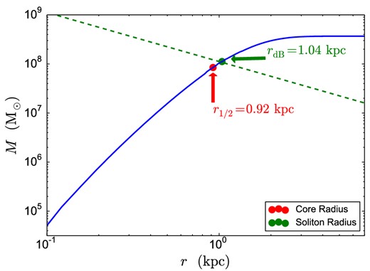
Solving equation (13). Blue: left-hand side, the mass of the soliton as a function of radius for some representative dwarf galaxy parameters. Green: right-hand side, the intersection solves for the de Broglie radius thus defined. The red dot shows the core radius as defined by Schive et al. (2014a), r_1/2, while the green dot shows the de Broglie radius obtained from the uncertainty principle. Because of the steeply falling soliton profile outside of the core, neither definition of core radius fixes the density of the point of transition to NFW accurately (Schive et al. 2014a,b).

Open in new tab Download slide

The form of the scaling in equation (9) is the same as for the halo Jeans scale extrapolated from linear theory (Hu et al. 2000; Marsh & Silk 2013; Guth et al. 2014). Both follow from the scale symmetry and dimensional analysis, and thus their interpretation as related to the de Broglie scale remains the same (see also Hlozek et al. 2015). Beyond scaling alone, how exactly are the linear Jeans scale and the soliton size related numerically? Can this be used to predict properties of axion haloes, including the core-size/mass relation, and the transition to NFW?

The simulation results of Schive et al. (2014a) indicate a soliton core connecting to an NFW profile at larger radii. No prescription for the matching radius is provided, however. In a follow up paper (Schive et al. 2014b), the same authors assessed halo formation in this model as the gravitational collapse of a system of solitons. Using the uncertainty principle and the virial theorem they motivated a relationship between the total halo mass, M_h, the soliton core mass M(< r_1/2), and the minimum halo mass, M_min: M(< r_1/2) ∝ (M_h/M_min)^1/3M_min.

Hu et al. (2000) and Marsh & Silk (2013) related the core radius to the halo Jeans scale. Can the same quantity be used to define a matching point between soliton and NFW? With respect to the linear Jeans scale r_J, the halo Jeans scale, r_{J, h}, satisfies

\begin{equation} \frac{\rho (r_{{\rm J,h}})}{\rho _{\rm crit}}=\left(\frac{r_{{\rm J}}}{r_{{\rm J,h}}}\right)^4 . \end{equation}

(14)

In order for this relation to define a matching point between soliton and NFW profiles, both profiles must provide a solution to this equation at the same radius. The logarithmic slope, Γ, of the NFW profile is in the range −3 < Γ < −1 and so there is always a single unique solution for r_{J, h}. However, the slope of the soliton profile is zero at the origin, decreasing to Γ < −4 at large radius. For the soliton, there can be either zero, one, or two solutions for r_{J, h}, with a single unique solution at the point where Γ = −4. Using the relationship in equation (8) it is possible to show that solutions only occur for δ_s ≪ 1. Haloes, on the other hand, correspond to non-linear density perturbations with δ_s ≫ 1. Therefore, the transition from soliton to NFW profile in a halo must occur on radii smaller than the linear Jeans scale extrapolated using the local density, i.e. on r < r_{J, h} defined by equation (14). This implies that soliton cores are more compact than expected from linear theory. This will turn out to have important implications for a possible solution to the cusp–core problem using ULAs/scalar field DM.

3 AXION HALO DENSITY PROFILES AND DWARF GALAXY CORES

In this section we will first define our proposal for the complete halo density profile of axion /scalar-field DM. We then go on to estimate the parameters in this profile using the Fornax and Sculptor dSph density profile slopes as measured by WP11. We introduce this measurement and the approximations it uses, define a likelihood from this, and perform a Monte Carlo Markov chain (MCMC) analysis. The results are all contained in Table 3 and Figs 2 and 3.

Figure 2.

Two and one-dimensional marginalized posteriors on the constrained density profile parameters for the HUDF mass prior (see Table 2). Contour levels show [0.5, 1.0, 1.5, 2.0]σ preferred regions. Vertical dashed lines show [0.05, 0.5, 0.95] percentiles. This plot is made using triangleplot (Foreman-Mackey 2014).

Open in new tab Download slide

Figure 3.

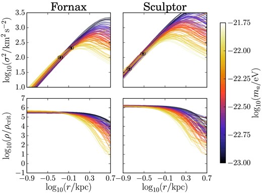
Velocity dispersions are estimated at the stellar half-light radii from M(< r_h), equation (19). We show velocity dispersions and density profiles of 200 random samples from our MCMC using the HUDF mass prior (see Table 2). The large core in Fornax favours low axion masses. Consistency with HUDF predicts a rapid turnover in the density slope at radii slightly larger than those observed, caused by the transition from soliton to NFW. Data from WP11, quoted in Table 1.

Open in new tab Download slide

3.1 Defining the density profile

The halo density profiles for ultralight scalar DM observed in the simulations of Schive et al. (2014a,b) consist of an NFW-like outer region, with a prominent solitonic core. The observed transition is sharp, and we model it as a step function:

\begin{equation} \rho (r)=\Theta (r_\epsilon -r)\rho _{\rm sol}(r)+\Theta (r-r_\epsilon )\rho _{\rm NFW}(r) . \end{equation}

(15)

The transition to an NFW profile at some radius is expected on a number of physical grounds. Axion/scalar field DM is indistinguishable from CDM on large scales, and this is the basis of the Schrödinger approach to simulating CDM (Widrow & Kaiser 1993; Uhlemann, Kopp & Haugg 2014). Thus, on scales much larger than the de Broglie wavelength, the scalar field haloes should resemble those found in N-body simulations, i.e. NFW. Furthermore, no long range correlation should occur; the smallest objects are solitons, with a characteristic granularity fixed by the Jeans scale (Guth et al. 2014; Schive et al. 2014a,b). On large scales, phase decoherence should occur, violating the assumption in our soliton ansatz that ∂_rγ = 0.

The dynamics will be that of an interacting gas of solitons in a decoherent scalar field background. On length scales larger than the soliton radius the usual thermodynamic arguments relating to dust (Binney & Tremaine 2008) will apply, leading to an NFW-like profile (on large scales this equivalence between the Schrödinger picture and dust thermodynamics can be derived using the Wigner distribution; e.g. Widrow & Kaiser 1993; Uhlemann et al. 2014). The transition in behaviour from soliton to NFW governed by the decoherence scale, and the mass function of solitons in the outer halo are all interesting questions, and will be the subjects of forthcoming papers. The NFW density profile is given by (Navarro, Frenk & White 1997)

\begin{equation} \frac{\rho _{\rm NFW}(r)}{\rho _{\rm crit}}=\frac{\delta _{\rm char}}{(r/r_{\rm s})(1+r/r_{\rm s})^2} . \end{equation}

(16)

We fit for the soliton density profile in Appendix A6:

\begin{equation} \frac{\rho _{\rm sol}(r)}{\rho _{\rm crit}} = \frac{\delta _{\rm s}}{(1+(r/r_{\rm sol})^2)^8} . \end{equation}

(17)

We take δ_s as a free parameter and r_sol is fixed in terms of it by equation (8) using α = 0.230. The rescaling parameter, λ, can then be found by setting r_sol = (λαm_a)⁻¹. We recall that consistent solutions with |γ/m| ≪ 1 require λ < 1, which also guarantees ϕ(0) ≲ 0.3M_pl and the stability of the soliton (Seidel & Suen 1990).

We match the soliton and NFW profiles at a fixed value of the overdensity, δ = ϵδ_s, defining the matching radius r_ϵ. Since we have not been able to find an accurate estimate that fixes ϵ analytically, we take it as a free parameter.³ Continuity of the density at this point fixes one of the two free parameters in the NFW profile. We choose this to be δ_char and take the scale radius to be a free parameter. For a given ULA mass, our halo density profile thus has three additional free parameters:

\begin{equation} \lbrace \delta _{\rm s},\epsilon ,r_{\rm s}\rbrace . \end{equation}

(18)

We emphasize again that a theoretical model for the value of ϵ, which could depend on redshift, central density, and/or particle mass, could perhaps be derived. In this case, the density profile has just as many free parameters as an NFW profile. Thus, in any given halo, a core measurement would predict the point of transition to NFW, and a measurement of the outer halo fixing concentration and scale radius would predict the corresponding inner core size.

The data we use imply cored profiles on the observed radii, and so in our phenomenological model with free ϵ we will find that the NFW parameters ϵ and r_s are unconstrained. This shows that the data prefer soliton cores to NFW profiles. For a complete Bayesian analysis, we include and marginalize over the NFW parameters in our constraints, as described in the next subsection.

3.2 Fitting to Fornax and Sculptor

While there are several ways of analysing the observed data, we will focus on the method used by WP11 who measured the slopes of dSph mass profiles directly from stellar spectroscopic data. They use the fact that some dSphs have been shown to have at least two stellar populations that are chemodynamically distinct (see e.g. Tolstoy et al. 2004; Battaglia et al. 2006, 2011). Measuring the half-light radii and velocity dispersions of two such populations in a dSph allows one to infer the slope of the mass profile. The method of WP11 has the advantage that it does not need to adopt any DM halo model a priori. Therefore the data can be used to test theoretical density profile models without having to run computationally expensive fits to the full stellar data for each value of the theoretical parameters.

We model the results of WP11 as providing two-dimensional Gaussian distributions for the half-light radii, r_{h, i}, and velocity dispersions, σ(r_{h, i}), for each of the two stellar populations, i, in Fornax and Sculptor. While the exact results display some covariance between σ and r_h the Gaussian approximation is far simpler to analyse, and accurate enough for the purposes of this study. This follows the approach taken by Lombriser & Peñarrubia (2015) for testing chameleon gravity using dSphs. The data we use are given in Table 1.

Table 1.

Open in new tab

Data used in this work, taken from WP11. We approximate the likelihoods to be two-dimensional uncorrelated Gaussians in log₁₀(r, σ) for each data point.

dSph	log₁₀(σ²/km² s⁻²)	Error	log₁₀(r/kpc)	Error
Fornax	2.00	0.05	−0.26	0.04
	2.32	0.04	−0.05	0.04
Sculptor	1.62	0.06	−0.78	0.04
	2.13	0.05	−0.52	0.04

dSph	log₁₀(σ²/km² s⁻²)	Error	log₁₀(r/kpc)	Error
Fornax	2.00	0.05	−0.26	0.04
	2.32	0.04	−0.05	0.04
Sculptor	1.62	0.06	−0.78	0.04
	2.13	0.05	−0.52	0.04

Table 1.

Open in new tab

Data used in this work, taken from WP11. We approximate the likelihoods to be two-dimensional uncorrelated Gaussians in log₁₀(r, σ) for each data point.

dSph	log₁₀(σ²/km² s⁻²)	Error	log₁₀(r/kpc)	Error
Fornax	2.00	0.05	−0.26	0.04
	2.32	0.04	−0.05	0.04
Sculptor	1.62	0.06	−0.78	0.04
	2.13	0.05	−0.52	0.04

dSph	log₁₀(σ²/km² s⁻²)	Error	log₁₀(r/kpc)	Error
Fornax	2.00	0.05	−0.26	0.04
	2.32	0.04	−0.05	0.04
Sculptor	1.62	0.06	−0.78	0.04
	2.13	0.05	−0.52	0.04

For our density profile the mass internal to any radius, M(< r), can be computed analytically (and so can the derivative of the mass, dM/dr). These are the only ingredients necessary in analysing this simplified version of the stellar kinematic data. The velocity dispersion at the stellar half-light radius obeys the following empirical relationship:

\begin{equation} \sigma ^2(r_{\rm h})=\frac{2\,G M(<r_{\rm h})}{5 r_{\rm h}} . \end{equation}

(19)

This relationship is related to the virial theorem, and is found by solving the Jeans equation and finding a ‘sweet spot’ where a wide variety of density and velocity profiles agree (including projection and anisotropy effects). In this work we do not perform a full Jeans analysis and use only this analytic relationship and the derived errors on it, following WP11.

The two-dimensional nature of the (r, σ) data can be accounted for using an effective one-dimensional error (e.g. Ma, Hinshaw & Scott 2013). If the data have central values |$(\bar{x},\bar{y})$| and standard deviations (Σ_x, Σ_y), then for a given model y = f(x) the effective one-dimensional error is given by

\begin{equation} \Sigma _{\rm eff}^2=\Sigma _y^2+\left(\frac{{\rm d}f(\bar{x})}{{\rm d}x}\right)^2\Sigma _x^2 . \end{equation}

(20)

The likelihood, |$\mathcal {L}$|⁠, can then be approximated as

\begin{equation} \mathcal {L} \propto \exp \left[\frac{-(f(\bar{x})-\bar{y})^2}{2\Sigma _{\rm eff}^2} \right] . \end{equation}

(21)

We use the data for Fornax and Sculptor with equal weight in the combined likelihood. The axion mass, m_a, is a global parameter which is the same for both Fornax and Sculptor. Our final model thus has seven parameters in total:

\begin{equation} \left\lbrace m_{\rm a},\delta _{\rm s}^{\rm F},\delta _{\rm s}^{\rm S},r_{\rm s}^{\rm F},r_{\rm s}^{\rm S},\epsilon ^{\rm S},\epsilon ^{\rm F}\right\rbrace , \end{equation}

(22)

with F and S labelling Fornax and Sculptor, respectively.

The priors on these parameters are given in Table 2. We take Jeffreys’, or ‘least information’, priors in a fixed range for all parameters. We will discuss our results in detail shortly, but mention here those aspects relevant to priors. We find that the NFW parameters (ϵ, r_s) are unconstrained. The priors on these parameters are therefore irrelevant in quoting marginalized constraints on other parameters and we take them extremely wide to explore all possibilities. We impose an upper bound on the ϵ prior of ϵ = 0.5, so that the match must occur outside the half-density radius, consistent with the simulation results of Schive et al. (2014a). As already mentioned, the fact that these parameters are unconstrained has physical meaning: our MCMC finds no peak corresponding to an NFW profile, and thus the data prefer soliton cores to NFW cusps. The central densities are well constrained and so the results are independent of the prior.

Table 2.

Open in new tab

Priors on our density profile parameters, where U(a, b) is the uniform distribution on [a, b]. The lower bound on the mass prior, X is given two different values: X_CMB = −25 (Hlozek et al. 2015) and X_HUDF = −23 (Bozek et al. 2015), referred to as CMB and HUDF priors, respectively.

Parameter	Prior
log₁₀(m_a/eV)	U(X, −19)
\|$\log _{10}\delta _{\rm s}^{\rm F,S}$\|	U(0, 10)
log₁₀ϵ^{F, S}	U( − 5, log₁₀0.5)
\|$\log _{10}(r_{\rm s}^{\rm F,S}/{\rm kpc})$\|	U(−1, 2)

Parameter	Prior
log₁₀(m_a/eV)	U(X, −19)
\|$\log _{10}\delta _{\rm s}^{\rm F,S}$\|	U(0, 10)
log₁₀ϵ^{F, S}	U( − 5, log₁₀0.5)
\|$\log _{10}(r_{\rm s}^{\rm F,S}/{\rm kpc})$\|	U(−1, 2)

Table 2.

Open in new tab

Priors on our density profile parameters, where U(a, b) is the uniform distribution on [a, b]. The lower bound on the mass prior, X is given two different values: X_CMB = −25 (Hlozek et al. 2015) and X_HUDF = −23 (Bozek et al. 2015), referred to as CMB and HUDF priors, respectively.

Parameter	Prior
log₁₀(m_a/eV)	U(X, −19)
\|$\log _{10}\delta _{\rm s}^{\rm F,S}$\|	U(0, 10)
log₁₀ϵ^{F, S}	U( − 5, log₁₀0.5)
\|$\log _{10}(r_{\rm s}^{\rm F,S}/{\rm kpc})$\|	U(−1, 2)

Parameter	Prior
log₁₀(m_a/eV)	U(X, −19)
\|$\log _{10}\delta _{\rm s}^{\rm F,S}$\|	U(0, 10)
log₁₀ϵ^{F, S}	U( − 5, log₁₀0.5)
\|$\log _{10}(r_{\rm s}^{\rm F,S}/{\rm kpc})$\|	U(−1, 2)

We find a one-sided constraint on the axion mass, and so the percentiles quoted depend on the prior for the lower bound. We take two such priors. The first uses the results of Hlozek et al. (2015), which place an approximate lower bound on ULAs to be all of the DM of m_a > 10⁻²⁵ eV. This is a very conservative lower bound and relies only on linear constraints from the cosmic microwave background (CMB). It is thus extremely reliable. Our alternative prior uses the results Bozek et al. (2015), which constrains m_a > 10⁻²³ eV at more than 8σ significance using Hubble Ultra-Deep Field (HUDF). While this is a very strong bound, it relies on more assumptions about the astrophysics of reionization and on the non-linear structure formation of ULAs. This HUDF bound is, however, still rather conservative compared to other constraints to ULAs using non-linear scales (e.g. Lyman α forest; Amendola & Barbieri 2006).

We evaluate the likelihood using emcee, an affine-invariant MCMC ensemble sampler (Foreman-Mackey et al. 2013). We use 200 ‘walkers’. Convergence is tested by evaluating the autocorrelation time, which is found to be |$\mathcal {O}(80)$| for each parameter. With 5000 steps per walker the likelihood is thus evaluated over many correlation times, giving many independent samples. We have used an ‘MCMC hammer’ (Foreman-Mackey et al. 2013) to crack a very simple parameter constraint nut, but this gives us a high degree of confidence in our results, and allows us to present them in a completely Bayesian fashion.

Our results are presented in Table 3, and shown for the HUDF priors in Fig. 2. As already mentioned, the NFW parameters (r_s, ϵ) are unconstrained, and so we do not show them. A weak constraint could be found on these parameters if one were to solve the full Jeans equation to fit the stellar kinematic data, rather than using only the empirical relationship equation (19). The constraint is caused by requiring a fixed enclosed mass at large radius. This consequently also imposes a weak lower bound on the axion mass to give a finite core radius, as in Schive et al. (2014a). Such an analysis is beyond the scope of this paper. Information about the total halo virial mass could also allow one to impose the core–halo relation of Schive et al. (2014b), introducing a degeneracy between r_s and ϵ.

Table 3.

Open in new tab

Posteriors on the constrained density profile parameters. The mass constraint is quoted for both the CMB and HUDF priors (see Table 2). Upper and lower errors on the central densities are given as the 16th and 84th percentiles and are quoted for the HUDF prior only (see text for discussion). The upper bound on the axion mass reflects the minimum core size consistent with observations.

Parameter	Posterior
(m_a/eV)_HUDF	<1.1 × 10⁻²² (95 per cent C.L.)
(m_a/eV)_CMB	<1.0 × 10⁻²² (95 per cent C.L.)
\|$\log _{10}\delta _{\rm s}^{\rm F}$\|	\|$5.55^{+0.06}_{-0.08}$\|
\|$\log _{10}\delta _{\rm s}^{\rm S}$\|	6.19 ± 0.05

Parameter	Posterior
(m_a/eV)_HUDF	<1.1 × 10⁻²² (95 per cent C.L.)
(m_a/eV)_CMB	<1.0 × 10⁻²² (95 per cent C.L.)
\|$\log _{10}\delta _{\rm s}^{\rm F}$\|	\|$5.55^{+0.06}_{-0.08}$\|
\|$\log _{10}\delta _{\rm s}^{\rm S}$\|	6.19 ± 0.05

Table 3.

Open in new tab

Posteriors on the constrained density profile parameters. The mass constraint is quoted for both the CMB and HUDF priors (see Table 2). Upper and lower errors on the central densities are given as the 16th and 84th percentiles and are quoted for the HUDF prior only (see text for discussion). The upper bound on the axion mass reflects the minimum core size consistent with observations.

Parameter	Posterior
(m_a/eV)_HUDF	<1.1 × 10⁻²² (95 per cent C.L.)
(m_a/eV)_CMB	<1.0 × 10⁻²² (95 per cent C.L.)
\|$\log _{10}\delta _{\rm s}^{\rm F}$\|	\|$5.55^{+0.06}_{-0.08}$\|
\|$\log _{10}\delta _{\rm s}^{\rm S}$\|	6.19 ± 0.05

Parameter	Posterior
(m_a/eV)_HUDF	<1.1 × 10⁻²² (95 per cent C.L.)
(m_a/eV)_CMB	<1.0 × 10⁻²² (95 per cent C.L.)
\|$\log _{10}\delta _{\rm s}^{\rm F}$\|	\|$5.55^{+0.06}_{-0.08}$\|
\|$\log _{10}\delta _{\rm s}^{\rm S}$\|	6.19 ± 0.05

For the central densities, shifts in the central values using the CMB prior compared to the HUDF prior are smaller than 1σ for Fornax and Sculptor, with comparable errors in both cases. The shift for Fornax is ever-so-slightly larger due to the degeneracy between δ_s and m_a enforced by equation (8) having an effect when marginalizing over m_a with a different prior in the unconstrained, low-mass region. The degeneracy between these parameters is more pronounced for Fornax as it is less cored than Sculptor. This same effect is the cause of the non-Gaussianity in the one-dimensional central density distribution for Fornax.

Random samples from our emcee runs showing the density and velocity profiles colour coded by axion mass are shown in Fig. 3 for the HUDF prior. This makes one clear point: since the HUDF prior already restricts the mass, cores cannot be too large. Therefore, if ULAs are responsible for dSph cores, velocity dispersions and density profiles must turn over quite rapidly on radii just larger than those observed. This is, in principle, a falsifiable prediction of the ULA model for cores.

4 DISCUSSION AND CONCLUSIONS

In this paper we have investigated stable solitonic density profiles, which are expected to be the smallest structures formed in models of axion/scalar field DM. We found these objects via numerical solution of the BVP in the Schrödinger approach to DM. Via use of a scaling symmetry we found a universal relationship between the central density of the soliton, the soliton radius, and the DM particle mass. We further explained the soliton size by recourse to the uncertainty principle. The standard thermodynamic arguments for dust, and the formal equivalence between the Schrödinger picture and dust on large scales, further supported by evidence from simulation, lead us to consider solitons as the central cores in NFW haloes. We presented a new phenomenological model for such a density profile.

If the DM is ultralight, then solitons may be responsible for the density cores observed in dSph galaxies, with soliton density profiles in the inner regions, and an outer NFW profile. We investigated the validity of this claim by performing an MCMC analysis of the simplified stellar kinematic data of WP11 for Fornax and Sculptor. This data shows a preference for cores over cusps, but other studies prefer cusps (e.g. Breddels & Helmi 2013; Richardson & Fairbairn 2014). The preference of the WP11 data for large cores shows up as an upper bound on the axion DM mass of m_a < 1.1 × 10⁻²² eV at 95 per cent C.L., leaving the NFW parameters unconstrained and marginalized over. The axion mass bound applies only if the dSph cores are solitonic, and not if they are caused by baryonic effects for standard CDM (be it composed of heavier axions, WIMPs, etc.). This bound is consistent with the best-fitting mass |$m_{\rm a}=8.1^{+1.6}_{-1.7}\times 10^{-23}{\rm \,eV}$| (an approximate 95 per cent C.L. region 0.47 ≲ m_a/10⁻²² eV ≲ 1.13) of Schive et al. (2014a) found by solving a simplified version of the full Jeans equations for a single stellar subcomponent in Fornax alone. Schive et al. (2014a) also checked the (rough) consistency of their results with density profile slope measurements, but our analysis is the first to use these data together in a complete and Bayesian manner. In future we hope to conduct a full Jeans analysis for our model, following the similar analysis for self-interacting scalar field DM by Diez-Tejedor, Gonzales-Morales & Profumo (2014).

The existence of an upper bound on the DM particle mass in the axion model has a number of interesting consequences. Structure formation in this model is substantially different from CDM due to the cut-off in the power spectrum on small scales caused by the axion sound speed and resulting Jeans scale. Bozek et al. (2015) found that, if the DM is composed entirely of ultralight axions, m_a = 10⁻²² eV is just consistent with HUDF. Our upper bound is right on the edge of this limit, and suggests two possible outcomes warranting further study.

Pessimistic. Structure formation and the requirement of dSph cores put conflicting demands on axion DM. This places the model in a ‘Catch 22’ analogous to WDM.⁴ This particle physics model is no longer a catch-all solution to the small-scale crises, and additional mechanisms are required for its consistency.
Optimistic. Ultralight axions are responsible for dSph cores. The cut-off in the power spectrum is just outside current observational reach. Near-future experiments will turn up striking evidence for axions in structure formation and in study of the high-z universe.

In the pessimistic case, axions have nothing to do with core formation in dSph galaxies, and another mechanism is needed to form the cores. The DM can still be composed of axions, but there is now no limit on the mass based on the dSph observations. Cores may be formed by baryonic processes, putting axion DM in the same situation as any other DM model, e.g. WIMPs. Cores could also be formed by adding strong self-interactions for CDM or for axions. One could also modify gravity, for example if the modulus partner of the axion played the role of a chameleon field (Khoury & Weltman 2004; Lombriser & Peñarrubia 2015). Another alternative would be to keep cores from axion solitons, but compensate structure formation by a boost in the primordial power or some other alteration to cosmology. A compensation based on a mixed DM model, however, is unlikely to succeed (Marsh & Silk 2013).

There are still opportunities to discover evidence for axion DM in the pessimistic case. We briefly outline some of these for the ‘most pessimistic’ case (from a particle physics view point) that cores are formed entirely by baryonic processes, and consider only searches influenced in some way by the Jeans scale or solitons, i.e. by non-trivial gravitational behaviour. For 10⁻²² ≲ m_a ≲ 10⁻²⁰ eV axions are consistent with current constraints from cosmology, but the cut-off in the power spectrum may still be observable using measurements of the weak lensing or 21-cm power spectra. Axions can further be evidenced by their effect on black holes via the super-radiant instability (Arvanitaki & Dubovsky 2011). Spinning supermassive black holes indirectly probe/constrain masses in the range 10⁻¹⁹ ≲ m_a ≲ 10⁻¹⁸ eV (Pani et al. 2012; Brito, Cardoso & Pani 2014). More direct signatures in gravitational wave detection may come from solar mass black holes for axions in the range 10⁻¹³ ≲ m_a ≲ 10⁻¹⁰ eV (Arvanitaki, Baryakhtar & Huang 2015).

Axion DM of any mass will contain solitons somewhere in the mass spectrum at some point in cosmic history. This could have a number of consequences relevant to both the optimistic and pessimistic scenarios outlined above. This model predicts small and dense cores in all DM haloes, with core size inversely related to central density and halo mass (equation 8; Schive et al. 2014b). Such cores may provide seeds for high-z quasars (Schive et al. 2014b). The granular nature of DM composed of solitons could be detected by measures of substructure (which we discuss further below). DM composed entirely of solitons/oscillons/boson stars may have a number of interesting features for gravitational wave observations, as discussed in, e.g. Evslin & Bjarke Gudnason (2012) and Macedo et al. (2013), that distinguish soliton DM from an equivalent model with black holes, due to the absence of a horizon. The soliton content of an axion DM halo will also impact the direct detection prospects (Hoskins et al. 2011), while the evaporation of solitons from axion self-interactions enhanced by the high number densities could have indirect signatures. Other signatures of the soliton components of an axion halo, e.g. in precision time-delay experiments with atomic clocks, may be similar to those with topological defect DM (Pospelov et al. 2013; Derevianko & Pospelov 2014; Stadnik & Flambaum 2014).

There are also ‘intermediate’ cases to consider. ULAs with m_a ≲ 10⁻²³ eV could be detected as a subdominant component of the DM with high precision studies (Hlozek et al. 2015). A subdominant component at these masses is likely the expectation based on string models with sub-Planckian axion decay constants (although see Bachlechner, Long & McAllister 2014). ULAs with m_a > 10⁻²² eV as the dominant DM could also play some role in core formation alongside inefficient baryonic processes.

Finally, we turn to discussion of the optimistic case, where axions at the edge of our allowed region in mass are solely responsible for dSph cores. In this case, soliton cores have a large mass |$\mathcal {O}(10^8\, \mathrm{M}_{\odot })$| and large radial extent |$\mathcal {O}(1{\rm \,kpc})$|⁠, and the cut-off in the halo mass function (in the field) occurs at M ∼ 10⁸ M_⊙ (the z = 0 Jeans mass; Marsh & Silk 2013; Bozek et al. 2015).

We have demonstrated the ability of soliton cores to fit the dSph observations, and suggested a complete density profile including the NFW piece. This density profile could be fit to many other observations, including rotation curves (de Blok et al. 2001; Robles & Matos 2012) and stellar clump survival (Lora & Magaña 2014). We argue that further study of this model should use the density profiles we advocate in this work, and not ‘multistate’ or other adaptations of the scalar field DM model. The outer NFW piece obviates the need for such additions, and is consistent with many lines of reasoning. Further study should, as we have in this work, account for consistency of the cosmology, as well as between different density profile constraints. Consistency with cosmology and our core size fits in this work suggest that density profiles just outside 1 kpc should be much steeper than cores and make a transition to NFW shortly thereafter. It should also be investigated whether the scale symmetry for soliton cores can be used to explain the observed scaling relationships in dwarf galaxies (Kormendy & Freeman 2014; Burkert 2015).

While density profiles provide the motivation for m_a ∼ 10⁻²² eV, cosmology suggests that the most striking evidence for such a model will be found in substructure and high-z galaxy formation. Measures of substructure from mililensing (Dalal & Kochanek 2002), tidal tails (Johnston, Spergel & Haydn 2002), and strong lensing (Hezaveh et al. 2014) should be sensitive to the absence of small-scale structure predicted by an axion solution to the cusp–core problem. Further study is required to formulate the predictions of the axion model in this regard. This should come from simulation, but also from semi-analytic study of the conditional mass function and extended Press–Schecter formalism (Lacey & Cole 1993). This study will further address the questions of whether axion DM can provide a consistent solution to other small-scale crises like ‘missing satellites’.

A final set of ‘smoking gun’ signatures in the optimistic scenario is suggested by the results of Bozek et al. (2015). Since m_a ∼ 10⁻²² eV is just consistent with the HUDF ultraviolet (UV) luminosity function, and also just able to provide a dSph core, this makes the prediction that a JWST measurement of the UV luminosity function sensitive to fainter magnitudes will only see a value consistent with HUDF, and not the larger value predicted by CDM. The cut-off in the mass function also makes predictions about reionization that are less sensitive to astrophysical uncertainties than in CDM. An axion solution to the cusp–core problem predicts that CMB polarization experiments (Calabrese et al. 2014) should measure: a low value of τ ∼ 0.05,⁵ a low redshift of reionization z_re ∼ 7, and thin width of reionization δz_re ∼ 1.5. These effects on reionization, caused by the rapid build up of massive structures at the mass function cut-off, should also turn up striking effects in the 21-cm power spectrum (building on Kadota et al. 2014; Sitwell et al. 2014). Further study of all of these signatures is underway.

We thank Niayesh Afshordi, Mustafa Amin, Asimina Arvanitaki, Avery Broderick, Tzihong Chiueh, Malcolm Faribairn, Renée Hlozek, Andrew Liddle, Eugene Lim, Ue-Li Pen, Gray Rybka, David Spergel, Clifford Taubes, Luis Ureña-Lopez, and Rosemary Wyse for helpful discussions. We especially thank Jorge Peñarrubia for help using the data from Walker & Peñarrubia (2011), the Royal Observatory of Edinburgh for hospitality, and Dan Grin for a careful reading of the manuscript. Research at Perimeter Institute is supported by the Government of Canada through Industry Canada and by the Province of Ontario through the Ministry of Research and Innovation.

1

Separating the function ψ(r, t) into polar coordinates in this way is sometimes referred to as the Madelung transformation (Madelung 1926).

2

Except the axion mass, which does not appear explicitly in equation (3), and hence only sets the units.

3

An order of magnitude estimate for the matching radius based on the de Broglie scale will not be enough. The soliton density falls rapidly for r > r_dB and so |$\mathcal {O}(1)$| numerical coefficients have a large effect on the estimate for ϵ.

4

Phrase coined by Macciò et al. (2012). For ULAs, one might call it a Catch 10⁻²².

5

In Bozek et al. (2015) it was noted that this is disfavoured at ∼2–3σ by WMAP (Bennett et al. 2013), however, it is in less tension with recent Planck results (Planck Collaboration XIII 2015).

6

Here, we are using a Schrödinger system as a change of variables to understand a classical wave equation, which also has a fluid description. Similarly, an understanding of classical fluids can help in understanding aspects of quantum mechanics. See Park (1979) for further discussion.

REFERENCES

Alcubierre

M.

de la Macorra

A.

Diez-Tejedor

A.

Torres

J. M.

2015

preprint (arXiv:1501.06918)

Amendola

L.

Barbieri

R.

Phys. Lett. B

2006

642

192

Crossref

Search ADS

Amendola

L.

et al.

Living Rev. Relativ.

2013

16

6

Crossref

Search ADS

Amin

M. A.

Phys. Rev. D

2013

87

123505

Crossref

Search ADS

Amin

M. A.

Easther

R.

Finkel

H.

Flauger

R.

Hertzberg

M. P.

Phys. Rev. Lett.

2012

108

241302

Crossref

Search ADS

PubMed

Arvanitaki

A.

Dubovsky

S.

Phys. Rev. D

2011

83

044026

Crossref

Search ADS

Arvanitaki

A.

Dimopoulos

S.

Dubovsky

S.

Kaloper

N.

March-Russell

J.

Phys. Rev. D

2010

81

123530

Crossref

Search ADS

Arvanitaki

A.

Baryakhtar

M.

Huang

X.

Phys. Rev. D

2015

91

084011

Crossref

Search ADS

Bachlechner

T. C.

Long

C.

McAllister

L.

2014

preprint (arXiv:1412.1093)

Banik

N.

Sikivie

P.

2015

preprint (arXiv:1501.05913)

Battaglia

G.

et al.

A&A

2006

459

423

Crossref

Search ADS

Battaglia

G.

Tolstoy

E.

Helmi

A.

Irwin

M.

Parisi

P.

Hill

V.

Jablonka

P.

MNRAS

2011

411

1013

Crossref

Search ADS

Bennett

C. L.

et al.

ApJS

2013

208

20

Crossref

Search ADS

Binney

J.

Tremaine

S.

Galactic Dynamics

2008

2nd edn

Princeton, NJ

Princeton Univ. Press

Google Scholar

Google Preview

OpenURL Placeholder Text

WorldCat

Bode

P.

Ostriker

J. P.

Turok

N.

ApJ

2001

556

93

Crossref

Search ADS

Boehm

C.

Fayet

P.

Schaeffer

R.

Phys. Lett. B

2001

518

8

Crossref

Search ADS

Bond

J. R.

Szalay

A. S.

Turner

M. S.

Phys. Rev. Lett.

1982

48

1636

Crossref

Search ADS

Boylan-Kolchin

M.

Bullock

J. S.

Kaplinghat

M.

MNRAS

2011

415

L40

Crossref

Search ADS

Bozek

B.

Marsh

D. J. E.

Silk

J.

Wyse

R. F. G.

MNRAS

2015

450

209

Crossref

Search ADS

Breddels

M. A.

Helmi

A.

A&A

2013

558

A35

Crossref

Search ADS

Brito

R.

Cardoso

V.

Pani

P.

2014

preprint (arXiv:1411.0686)

Burkert

A.

ApJ

2015

submitted (arXiv:1501.06604)

Calabrese

E.

et al.

J. Cosmol. Astropart. Phys.

2014

08

010

Crossref

Search ADS

Choptuik

M. W.

Phys. Rev. Lett.

1993

70

9

Crossref

Search ADS

PubMed

Coles

P.

2003

preprint (astro-ph/0209576)

Coles

P.

Spencer

K.

MNRAS

2003

342

176

Crossref

Search ADS

Dalal

N.

Kochanek

C. S.

ApJ

2002

572

25

Crossref

Search ADS

Davidson

S.

Astropart. Phys.

2015

65

101

Crossref

Search ADS

Davidson

S.

Elmer

M.

J. Cosmol. Astropart. Phys.

2013

12

34

Crossref

Search ADS

de Blok

W. J. G.

McGaugh

S. S.

Bosma

A.

Rubin

V. C.

ApJ

2001

552

L23

Crossref

Search ADS

Del Popolo

A.

ApJ

2009

698

2093

Crossref

Search ADS

Derevianko

A.

Pospelov

M.

Nat. Phys.

2014

10

933

Crossref

Search ADS

Diez-Tejedor

A.

Gonzales-Morales

A. X.

Profumo

S.

Phys. Rev. D

2014

90

043517

Crossref

Search ADS

Duffy

L. D.

et al.

Phys. Rev. D

2006

74

012006

Crossref

Search ADS

Elbert

O. D.

Bullock

J. S.

Garrison-Kimmel

S.

Rocha

M.

Oñorbe

J.

Peter

A. H. G.

2014

preprint (arXiv:1412.1477)

Evslin

J.

Bjarke Gudnason

S.

2012

preprint (arXiv:1202.0560)

Foreman-Mackey

D.

Hogg

D. W.

Lang

D.

Goodman

J.

PASP

2013

125

306

Crossref

Search ADS

Foreman-Mackey

D.

Hogg

D. W.

Morton

T. D.

ApJ

2014

795

64

Governato

F.

et al.

MNRAS

2012

422

1231

Crossref

Search ADS

Guth

A. H.

Hertzberg

M. P.

Prescod-Weinstein

C.

2014

preprint (arXiv:1412.5930)

Guzman

F. S.

Urena-Lopez

L. A.

Phys. Rev. D

2004

69

124033

Crossref

Search ADS

Guzmán

F. S.

Ureña-López

L. A.

ApJ

2006

645

814

Crossref

Search ADS

Hezaveh

Y.

Dalal

N.

Holder

G.

Kisner

T.

Kuhlen

M.

Perreault Levasseur

L.

ApJ

2014

submitted (arXiv:1403.2720)

Hlozek

R.

Grin

D.

Marsh

D. J. E.

Ferreira

P. G.

Phys. Rev. D

2015

91

103512

Crossref

Search ADS

Hoskins

J.

et al.

Phys. Rev. D

2011

84

121302

Crossref

Search ADS

Hu

W.

ApJ

1998

506

485

Crossref

Search ADS

Hu

W.

Barkana

R.

Gruzinov

A.

Phys. Rev. Lett.

2000

85

1158

Crossref

Search ADS

PubMed

Hwang

J.-C.

Noh

H.

Phys. Lett. B

2009

680

1

Crossref

Search ADS

Johnston

K. V.

Spergel

D. N.

Haydn

C.

ApJ

2002

570

656

Crossref

Search ADS

Johnston

R.

Lasenby

A. N.

Hobson

M. P.

MNRAS

2010

402

2491

Crossref

Search ADS

Jungman

G.

Kamionkowski

M.

Griest

K.

Phys. Rep.

1996

267

195

Crossref

Search ADS

Kadota

K.

Mao

Y.

Ichiki

K.

Silk

J.

J. Cosmol. Astropart. Phys.

2014

06

11

Crossref

Search ADS

Khlopov

M. I.

Malomed

B. A.

Zeldovich

I. B.

MNRAS

1985

215

575

Crossref

Search ADS

Khoury

J.

Weltman

A.

Phys. Rev. D

2004

69

044026

Crossref

Search ADS

Kim

J. E.

Phys. Rep.

1987

150

1

Crossref

Search ADS

Klypin

A.

Kravtsov

A. V.

Valenzuela

O.

Prada

F.

ApJ

1999

522

82

Crossref

Search ADS

Kormendy

J.

Freeman

K. C.

ApJ

2014

submitted (arXiv:1411.2170)

Lacey

C.

Cole

S.

MNRAS

1993

262

627

Crossref

Search ADS

Laureijs

R.

et al.

2011

preprint (arXiv:1110.3193)

Liddle

A. R.

Madsen

M. S.

Int. J. Modern Phys. D

1992

1

101

Crossref

Search ADS

Liebling

S. L.

Palenzuela

C.

Living Rev. Relativ.

2012

15

6

Crossref

Search ADS

Loeb

A.

Zaldarriaga

M.

Phys. Rev. D

2005

71

103520

Crossref

Search ADS

Lombriser

L.

Peñarrubia

J.

Phys. Rev. D

2015

91

084022

Crossref

Search ADS

Lora

V.

Magaña

J.

J. Cosmol. Astropart. Phys.

2014

9

11

Crossref

Search ADS

Lozanov

K. D.

Amin

M. A.

Phys. Rev. D

2014

90

083528

Crossref

Search ADS

Ma

Y.-Z.

Hinshaw

G.

Scott

D.

ApJ

2013

771

137

Crossref

Search ADS

Macciò

A. V.

Paduroiu

S.

Anderhalden

D.

Schneider

A.

Moore

B.

MNRAS

2012

424

1105

Crossref

Search ADS

Macedo

C. F.

Pani

P.

Cardoso

V.

Crispino

L. C. B.

Phys. Rev. D

2013

88

064046

Crossref

Search ADS

Madelung

E.

Z. Phys.

1926

40

332

Marsh

D. J. E.

Silk

J.

MNRAS

2013

437

2652

Crossref

Search ADS

Moore

B.

Ghigna

S.

Governato

F.

Lake

G.

Quinn

T.

Stadel

J.

Tozzi

P.

ApJ

1999

524

L19

Crossref

Search ADS

Navarro

J. F.

Frenk

C. S.

White

S. D.

ApJ

1997

490

493

Crossref

Search ADS

Noh

H.

Park

C.-G.

Hwang

J.-c.

Phys. Lett. B

2013

726

559

Crossref

Search ADS

Pani

P.

Cardoso

V.

Gualtieri

L.

Berti

E.

Ishibashi

A.

Phys. Rev. Lett.

2012

109

131102

Crossref

Search ADS

PubMed

Park

D.

Classical Dynamics and Its Quantum Analogues

1979

Berlin

Springer-Verlag

Google Scholar

Google Preview

OpenURL Placeholder Text

WorldCat

Peccei

R. D.

Quinn

H. R.

Phys. Rev. Lett.

1977

38

1440

Crossref

Search ADS

Peebles

P. J. E.

ApJ

2000

534

L127

Crossref

Search ADS

Planck Collaboration XVI

A&A

2014

571

A16

Crossref

Search ADS

Planck Collaboration XIII

2015

preprint (arXiv:1502.01589)

Pontzen

A.

Governato

F.

Nature

2014

506

171

Crossref

Search ADS

PubMed

Pospelov

M.

Pustelny

S.

Ledbetter

M. P.

Kimball

D. F. J.

Gawlik

W.

Budker

D.

Phys. Rev. Lett.

2013

110

021803

Crossref

Search ADS

PubMed

Richardson

T.

Fairbairn

M.

MNRAS

2014

441

1584

Crossref

Search ADS

Robles

V. H.

Matos

T.

MNRAS

2012

422

282

Crossref

Search ADS

Ruffini

R.

Bonazzola

S.

Phys. Rev.

1969

187

1767

Crossref

Search ADS

Schive

H.-Y.

Chiueh

T.

Broadhurst

T.

Nat. Phys.

2014a

10

496

Crossref

Search ADS

Schive

H.-Y.

Liao

M.-H.

Woo

T.-P.

Wong

S.-K.

Chiueh

T.

Broadhurst

T.

Hwang

W.-Y. P.

Phys. Rev. Lett.

2014b

113

261302

Crossref

Search ADS

Schneider

A.

Anderhalden

D.

Macciò

A. V.

Diemand

J.

MNRAS

2014

441

L6

Crossref

Search ADS

Seidel

E.

Suen

W.-M.

Phys. Rev. D

1990

42

384

Crossref

Search ADS

Seidel

E.

Suen

W.-M.

Phys. Rev. Lett.

1994

72

2516

Crossref

Search ADS

PubMed

Sikivie

P.

Yang

Q.

Phys. Rev. Lett.

2009

103

111301

Crossref

Search ADS

PubMed

Sitwell

M.

Mesinger

A.

Ma

Y.-Z.

Sigurdson

K.

MNRAS

2014

438

2664

Crossref

Search ADS

Smith

R. E.

Markovic

K.

Phys. Rev. D

2011

84

063507

Crossref

Search ADS

Spergel

D. N.

Steinhardt

P. J.

Phys. Rev. Lett.

2000

84

3760

Crossref

Search ADS

PubMed

Stadnik

Y. V.

Flambaum

V. V.

Phys. Rev. Lett.

2014

113

151301

Crossref

Search ADS

PubMed

Strigari

L. E.

Frenk

C. S.

White

S. D. M.

2014

preprint (arXiv:1406.6079)

Svrcek

P.

Witten

E.

J. High Energy Phys.

2006

06

051

Crossref

Search ADS

Tolstoy

E.

et al.

ApJ

2004

617

L119

Crossref

Search ADS

Uhlemann

C.

Kopp

M.

Haugg

T.

Phys. Rev. D

2014

90

023517

Crossref

Search ADS

Walker

M. G.

Peñarrubia

J.

ApJ

2011

742

20

(WP11)

Crossref

Search ADS

Weinberg

S.

Phys. Rev. Lett.

1978

40

223

Crossref

Search ADS

Widrow

L. M.

Kaiser

N.

ApJ

1993

416

L71

Crossref

Search ADS

Wilczek

F.

Phys. Rev. Lett.

1978

40

279

Crossref

Search ADS

Windhorst

R. A.

Cohen

S. H.

Jansen

R. A.

Conselice

C.

Yan

H.

New Astron. Rev.

2006

50

113

Crossref

Search ADS

Wyse

R. F. G.

Gilmore

G.

Davies

J. I.

Disney

M. J.

Proc. IAU Symp. 244, Dark Galaxies and Lost Baryons

2008

Cambridge

Cambridge Univ. Press

44

Google Scholar

Google Preview

OpenURL Placeholder Text

WorldCat

APPENDIX A: THE SCHRÖDINGER–POISSON SYSTEM

A1 Derivation

We begin by deriving our workhorse system, the Schödinger–Poisson (SP) form of the field equations, following Widrow & Kaiser (1993). Further reading on this formalism can be found in Coles (2003), Coles & Spencer (2003), Johnston, Lasenby & Hobson (2010), and references therein.⁶ The SP system can be viewed as a fundamental picture of structure formation for axions or other scalar DM, or as a numerical procedure to model and study CDM with a suitable cut-off, having certain advantages over N-body simulations (Uhlemann et al. 2014).

The Klein–Gordon (KG) equation for a free homogeneous scalar field ϕ of mass m_a, in an expanding universe with Hubble rate H, is

\begin{equation} \ddot{\phi } + 3H \dot{\phi } + \frac{c^4m_{\rm a}^2}{\hbar ^2} \phi = 0 . \end{equation}

(A1)

From this point onwards, we will set c = 1, but keep factors of ℏ for now. In the regime H ≪ m (valid at late times, when the axion field is oscillating and behaving as DM) the equation above can be solved by WKB methods,

\begin{equation} \phi = \frac{\hbar }{\sqrt{2} \, m_{\rm a}} (\psi \, {\rm e}^{-{\rm i}mt/\hbar } + \psi ^* {\rm e}^{{\rm i}mt/\hbar }) , \end{equation}

(A2)

for the function ψ that is slowly varying with time, i.e. |$|m \, \psi | \gg |\hbar \, \dot{\psi }|$|⁠.

The time–time metric component is (in the Newtonian gauge and in physical time)

\begin{equation} g_{00} = - [1+2V(r)] , \end{equation}

(A3)

where V(r) is the Newtonian potential. Treating this perturbatively, the KG equation for the inhomogeneous field becomes

\begin{equation} \frac{1}{\sqrt{-g}} \mathrm{\partial} _\mu \left[ \sqrt{-g} g^{\mu \nu } \mathrm{\partial} _\nu \right] \phi - \frac{m_{\rm a}^2}{\hbar ^2} \phi = 0 , \end{equation}

(A4)

\begin{equation} \ddot{\phi } + 3H\dot{\phi } - \mathrm{\partial} ^i \mathrm{\partial} _i \phi + (1+2V) \frac{m_{\rm a}^2}{\hbar ^2} \phi =0 . \end{equation}

(A5)

In the non-relativistic limit, this equation has the same ansatz solution as the homogeneous field equation. Plugging in our ansatz and neglecting terms of order |$O(\ddot{\psi })$|⁠, since ψ is a slowly varying function of time, we find

\begin{eqnarray} \ddot{\phi } &= &\sqrt{2}i \left( -\dot{\psi } {\rm e}^{-{\rm i}m_{\rm a}t/\hbar } + \dot{\psi }^* {\rm e}^{{\rm i}m_{\rm a}t/\hbar } \right) \nonumber \\ &&- \frac{m}{\sqrt{2}\hbar } \left( \psi \, {\rm e}^{-{\rm i}m_{\rm a}t/\hbar } + \psi ^* {\rm e}^{{\rm i}m_{\rm a}t/\hbar } \right) , \end{eqnarray}

(A6)

\begin{equation} \nabla ^2 \phi = \frac{\hbar }{\sqrt{2}m_{\rm a}} \left( \nabla ^2 \psi \, {\rm e}^{-{\rm i}m_{\rm a}t/\hbar } + \nabla ^2 \psi ^* {\rm e}^{{\rm i}m_{\rm a}t/\hbar } \right) . \end{equation}

(A7)

In the regime H ≪ m, the second term in equation (A5) can be neglected. This gives

\begin{eqnarray} &&{\sqrt{2} \, i\, (- \dot{\psi } \, {\rm e}^{-{\rm i}m_{\rm a}t/\hbar } \!+\! \dot{\psi }^* {\rm e}^{{\rm i}m_{\rm a}t/\hbar })} \nonumber \\ &&-\frac{\hbar }{\sqrt{2} m} \left( \nabla ^2 \psi \, {\rm e}^{-{\rm i}m_{\rm a}t/\hbar } \!+\! \nabla ^2 \psi ^* {\rm e}^{{\rm i}m_{\rm a}t/\hbar } \right) \nonumber \\ && +2V \frac{m}{\sqrt{2}\hbar } \left( \psi \, {\rm e}^{-{\rm i}m_{\rm a}t/\hbar } + \psi ^* {\rm e}^{{\rm i}m_{\rm a}t/\hbar } \right) = 0 . \end{eqnarray}

(A8)

Multiplying the equation above by |$\hbar /\sqrt{2}$| and identifying all terms with the same exponential factor, we find the familiar Schrödinger equation:

\begin{equation} i\hbar \dot{\psi } = - \frac{\hbar ^2}{2m}\nabla ^2 \psi + m_{\rm a}V \psi . \end{equation}

(A9)

In the subhorizon, non-relativistic limit, in any gauge, the Poisson equation is

\begin{equation} \nabla ^2 V = 4 \pi G \rho = 4 \pi G \psi \psi ^* . \end{equation}

(A10)

Equations (A9) and (A10) form the coupled SP system for inhomogeneous scalar fields, give as equation (1). The non-relativistic limit in this case caused us to drop the gradient energy from the right-hand side of the Poisson equation, setting ρ = |ψ|². This is valid in the limit that k/m_a ≪ 1 for wavenumber k, i.e. ∂_xϕ/(M_plm_a) ≪ 1. Consistent solutions to the SP system must respect this limit.

In deriving this form of the field equations, the only quantity that has been treated perturbatively is the potential, V, i.e. we are working in the weak-field, Newtonian limit of general relativity. We have not treated the field, ϕ, or the density, ρ, perturbatively, and therefore our results will be valid in the non-linear (in terms of density fluctuations about the critical density) regime of gravitational collapse. The only clear limitation of our solutions will be instability to black hole formation: the Jeans limit (for boson stars, this is the analogue of the Chandrasekhar limit; see Ruffini & Bonazzola 1969; Khlopov et al. 1985; Seidel & Suen 1990; Choptuik 1993, for more details).

The SP system is simply another way of rewriting the KG equation, and is related to the more familiar fluid treatment of scalar fields in cosmology (e.g. Hu 1998). The standard fluid picture is most useful for studying linear perturbations in Fourier space via the sound speed and Jeans instability (e.g. Hwang & Noh 2009; Noh, Park & Hwang 2013; Hlozek et al. 2015; Alcubierre et al. 2015). We will find the Schrödinger picture to be more intuitive and useful for applications in real space relevant to non-linear densities in haloes.

A2 Dimensionless variables

Plugging the soliton ansatz, equation (2), into the SP system, equations (1), yields

\begin{eqnarray} \nabla ^2 \chi &=& \frac{2m_{\rm a}^2}{\hbar ^2}\left(V - \hbar \frac{\gamma }{m_{\rm a}}\right) \chi , \nonumber \\ \nabla ^2 V &=& 4 \pi G \chi ^2 . \end{eqnarray}

(A11)

From equation (A2), we know the dimension of [χ] = [ψ] = [m_a][ϕ] = [m_a]², and we will now replace χ, r, and γ by the dimensionless variables |$\tilde{\chi }$|⁠, |$\tilde{r}$|⁠, and |$\tilde{\gamma }$|⁠:

\begin{eqnarray} &&{\chi \rightarrow \tilde{\chi } \, m_{\rm a} M_{{\rm pl}} \sqrt{2}\left(\frac{c}{\hbar }\right)^{3/2}\rightarrow \tilde{\chi } m_{\rm a} \frac{c^2}{\hbar }\frac{1}{\sqrt{4\pi G}} ,} \nonumber \\ &&r \rightarrow \tilde{r} \, \hbar /m_{\rm a}c , \nonumber \\ &&\gamma \rightarrow \tilde{\gamma } \, m_{\rm a}/\hbar . \end{eqnarray}

(A12)

In these dimensionless variables the SP system is

\begin{eqnarray} \tilde{\nabla }^2 \tilde{\chi } &=& 2\left(V - \tilde{\gamma }\right) \tilde{\chi }, \end{eqnarray}

(A13)

\begin{eqnarray} \tilde{\nabla }^2V &=& \tilde{\chi }^2 . \end{eqnarray}

(A14)

Tildes can then be dropped.

A3 Scaling relations

The SP system of equations (3) obeys a scaling relation (r, χ, V, γ) → (r/λ, λ²χ, λ²V, λ²γ) for scale factor λ (Ruffini & Bonazzola 1969). This is easy to check:

\begin{eqnarray*} \nabla ^2 \chi &=&Y \frac{1}{\lambda ^2} \nabla ^2 \tilde{\chi } = \frac{1}{\lambda ^4} \tilde{\nabla }^2 \tilde{\chi } , \nonumber \\ 2(V-\gamma )\chi &=& 2\frac{(\tilde{V} - \tilde{\gamma })}{\lambda ^2} \frac{\tilde{\chi }}{\lambda ^2} , \nonumber \\ \nabla ^2\chi &=& 2(V - \gamma )\chi , \nonumber \\ \Leftrightarrow \; \; \frac{1}{\lambda ^4} \tilde{\nabla }^2\tilde{\chi } &=& \frac{2}{\lambda ^4}(\tilde{V}-\tilde{\gamma })\tilde{\chi }, \nonumber \\ \Leftrightarrow \; \; \tilde{\nabla }^2\tilde{\chi } &=& 2(\tilde{V}-\tilde{\gamma })\tilde{\chi } . \nonumber \end{eqnarray*}

We can also extend this scaling relation to include the mass of the soliton:

\begin{eqnarray} M_{\rm s} &=& \int _0^{r_{\rm s}}4\pi r^2 \rho \, \mathrm{d}r = \int _0^{r_{\rm s}}4\pi r^2 |\chi |^2 \mathrm{d}r \nonumber \\ &=& \int _0^{\tilde{r}_{\rm s}}4\pi r^2 \frac{|\tilde{\chi }|^2}{\lambda ^4} \lambda ^3 \mathrm{d}\tilde{r} = \frac{\tilde{M_{\rm s}}}{\lambda } , \end{eqnarray}

(A15)

and the density of the soliton:

\begin{equation} \rho _{\rm sol} = |\chi |^2 = \frac{1}{\lambda ^4}|\tilde{\chi }|^2 = \frac{\tilde{\rho }_{\rm sol}}{\lambda ^4}. \end{equation}

(A16)

Therefore, we can summarize the scaling relation as

\begin{equation} (r, \chi , V, \gamma , M_{\rm s}, \rho _{\rm s}) \rightarrow (r/\lambda , \lambda ^2 \chi , \lambda ^2 V, \lambda ^2\gamma ,\lambda M_{\rm s}, \lambda ^4 \rho _{\rm s}). \end{equation}

(A17)

This scaling symmetry is very powerful, and makes results about the small-scale clustering of axion/scalar-field DM have a universal character. The scaling can be used to find the density profiles on different length and density scales at fixed axion mass, m_a, but can also be used to rescale the mass at fixed length scale. The scaling symmetry will be useful to us in Appendix A5, where we numerically find soliton solutions with arbitrary central density ρ and then scale them to astrophysical densities.

For the SP system to be used as a model for the gravitational collapse of non-relativistic DM axions, its solutions must be consistent limits of the full KG equation satisfying γ ≪ 1 and k/m ≪ 1. Solutions to the SP system for a fixed scaling are formally solutions regardless of the value of γ and need not satisfy these constraints. However, when we fix the scaling for real astrophysical systems, the rescaled values must satisfy these constraints. In typical DM haloes, the virial velocity is v ∼ 100 km s⁻¹ ≪ c. Since both γ and k are related to the kinetic energy, we therefore expect to find these limits satisfied in astrophysical objects. In our explicit examples of density profiles for dSphs this is indeed the case.

A4 Power-law solutions

In this subsection, we are especially interested in the oscillaton profile at small radii. In the limit r → 0, we can assume that the dominant term in the series expansion of the solution χ(r) is of the form χ = Cr^β, for a given constant C and exponent β to be determined below.

In the case β ≠ {−1, 0} the Schrödinger equation implies:

\begin{eqnarray} \chi ^{\prime \prime } + 2\frac{\chi ^{\prime }}{r} &=& \beta (\beta + 1) C r^{\beta -2} , \nonumber \\ &=& 2(V-\gamma ) C r^\beta . \end{eqnarray}

(A18)

Therefore, as r → 0, we find that V(r) obeys the equation:

\begin{equation} V - \gamma = \frac{\beta (\beta +1)}{2r^2}. \end{equation}

(A19)

Substituting into the Poisson equation:

\begin{eqnarray*} V^{\prime \prime } + 2\frac{V^{\prime }}{r} &=& C^2 r^{2\beta }, \nonumber \\ 3\beta \frac{(\beta +1)}{r^4} - 2\beta \frac{(\beta +1)}{r^4} &=& C^2 r^{2\beta }, \nonumber \\ \beta (\beta +1) &=& C^2 r^{2\beta +4}, \end{eqnarray*}

we find that the SP system has a solution for β = −2. This implies a steeply increasing central density profile:

\begin{equation} \rho (r) = \chi ^2(r) \sim r^{-4}. \end{equation}

(A20)

However, in this case, we can see that the mass within any radius r_c diverges:

\begin{equation} M = \int _0^{r_{\rm c}} \rho (r) 4 \pi r^2 \mathrm{d}r \sim 4 \pi \left( - \frac{1}{r} \right)\bigg |_0^{r_{\rm c}} \rightarrow \infty . \end{equation}

(A21)

Therefore, the requirement that the central mass is finite excludes the case β = −2 .

Next we check the cases β = 0 and β = −1 separately.

For β = −1, we have that χ = C/r, χ^′ = −C/r², χ^′^′ = 2C/r³, and thus

\begin{equation*} \chi ^{\prime \prime } + 2\frac{\chi ^{\prime }}{r} = 2\frac{C}{r^3} - 2\frac{C}{r^3} = 0 = 2(V-\gamma ) \frac{C}{r} . \nonumber \end{equation*}

This expression must be true as r → 0, and therefore, it imposes that lim_{r → 0}V = γ. In this case, the Poisson equation becomes

\begin{equation*} V^{\prime \prime } + 2\frac{V^{\prime }}{r} = \frac{C^2}{r^2} , \end{equation*}

with V = log(r) a solution of the equation, for a constant |$C = \sqrt{3}$|⁠.

Thus, the SP system allows solutions with β = −1, i.e. solutions of the form |$\lim _{r \rightarrow 0} \chi = \sqrt{3}/r$|⁠. Unlike the β = −2 case, these solutions will have a finite mass. Nevertheless, solutions with β = −1 are non-physical because they correspond to infinite total energy:

\begin{eqnarray*} E &=& \int _0^{r_{\rm c}} (\nabla \chi )^2 4 \pi r^2 \mathrm{d}r \nonumber \\ &=& \int _0^{r_{\rm c}} \frac{3}{r^4} 4 \pi r^2 \mathrm{d}r \sim 12 \pi \left(-\frac{1}{r}\right) \bigg |_0^{r_{\rm c}} \rightarrow \infty . \nonumber \end{eqnarray*}

Finally, for β = 0, we must also consider the next terms in the expansion of χ(r) at small radii (i.e. |$\chi (r) = C_0 + C_1 r^{\beta _1} +\cdots$| with β_i > 0). If all the coefficients of terms with positive powers of r are zero, we recover the trivial solution χ(r) = C at all radii. This trivial homogeneous solution corresponds to the background density and the global ground state. We can also have non-trivial solutions for which the dominant term in the expansion at r → 0 is a constant and the higher order terms have non-zero coefficients. The numerical solution to the boundary value problem (BVP) with V(r → ∞) = χ(r → ∞) = 0 found in Appendix A5 is such a solution. It has lim_{r → 0}χ^′ = 0 , while the boundary conditions forbid the global ground state and enforce lim_{r → 0}χ^′^′ < 0 .

The solutions with β = −1 and β = −2 are clearly not solutions that minimize the total energy, so they cannot represent the local ground state. Also, each violates the non-relativistic condition, k/m ≪ 1, which in dimensionless variables and spherical coordinates reads ∂_rχ ≪ 1. These solutions are not consistent limits of the fundamental EKG equations. The existence of these solutions does, however, point to the instability of the r⁰ flat-core (pseudo) soliton. The instability, however, is a relativistic one, and the SP system is not suitable to analyse it. The solutions become relativistic before the β = −1 or β = −2 solutions are ever found, and a black hole will form for finite mass and energy. The flat-core soliton solution is unstable to black hole formation when the central field value exceeds ϕ(0) ≳ 0.3M_pl (Seidel & Suen 1990). This fixes the maximum, Chandrasekhar-like, soliton mass as a function of m_a (Ruffini & Bonazzola 1969).

The result that the consistent, non-relativistic density profiles are flat as r → 0 is not surprising given that we were analysing solitons, which are by definition spatially confined, non-dispersive and non-singular solutions of a non-linear field theory.

A5 Numerical solutions

The SP system found in equation (3) does not have an analytic solution. We devote this section to finding the soliton profile for the SP system numerically.

A5.1 Boundary conditions

We begin by noting that the SP system consists of two second-order ODEs with an additional unknown parameter γ, and thus we need to set five boundary conditions such that the system is uniquely determined. In Section A4 for χ ∼ r^β as r → 0 we found that β = 0 and therefore, χ^′(0) = 0. In addition, we are always free to normalize χ such that χ(0) = 1, and then later restore units and use the scaling symmetry to ensure that χ(0)² matches the desired central density. Two additional boundary conditions can be set by imposing a vanishing density and potential far away from the core (i.e. χ(r → ∞) = 0 and V(r → ∞) = 0). Thus, the first four boundary conditions arise naturally, and we are only left with the task of finding one more. This last condition arises from the fact that χ^′(0) = χ^′^′(0) = 0 when we have a flat core (i.e. β = 0). Then, by differentiating the Schrödinger equation with respect to r, we have

\begin{equation} \chi ^{\prime \prime \prime } + 2\frac{\chi ^{\prime \prime }}{r} - 2\frac{\chi ^{\prime }}{r^2} = 2V^{\prime } + 2(V-\gamma ) \chi ^{\prime } \end{equation}

(A22)

\begin{equation} \Rightarrow V^{\prime }(r\rightarrow 0) = 0. \end{equation}

(A23)

Thus, in order to find the soliton profile, we need to solve the BVP:

\begin{eqnarray} \chi ^{\prime \prime } + \frac{2\chi ^{\prime }}{r} &=& 2(V-\gamma )\chi , \end{eqnarray}

(A24)

\begin{eqnarray} V^{\prime \prime } + \frac{2V^{\prime }}{r} &=& \chi ^2, \end{eqnarray}

(A25)

with boundary conditions:

\begin{eqnarray} \chi (0) = 1, \end{eqnarray}

(A26)

\begin{eqnarray} \chi ^{\prime }(0) = 0, \end{eqnarray}

(A27)

\begin{eqnarray} \chi (\infty ) = 0, \end{eqnarray}

(A28)

\begin{eqnarray} V^{\prime }(0) = 0, \end{eqnarray}

(A29)

\begin{eqnarray} V(\infty ) = 0. \end{eqnarray}

(A30)

BVPs which have one or more of the boundary conditions set at infinity are inherently difficult to solve numerically. One can attempt to replace the boundary at infinity by a boundary at r = R ≫ 1, but this method will be very sensitive to the choice of R and, in most cases, will fail to converge to the exact solution of the BVP. Instead, we note that χ (r → ∞) = 0 and V (r → ∞) = 0, and by assuming that γ is not too small (i.e. V(R) ≪ |γ| for R ≫ 1), we can approximate the SP system as follows:

\begin{eqnarray} \chi ^{\prime \prime } + 2\frac{\chi ^{\prime }}{r} &=& 2(V-\gamma )\chi , \end{eqnarray}

(A31)

\begin{eqnarray} \chi ^{\prime \prime }(R \gg 1) &\approx& -2\, \gamma \, \chi \,(R\gg 1), \end{eqnarray}

(A32)

so at large values of R,

\begin{equation} \chi (R) \propto {\rm e}^{-\sqrt{- 2 \gamma } R} \; \; \; \mathrm{for\; \; \; } \gamma < 0. \end{equation}

(A33)

We expect γ < 0 because χ must decay at large distances, whilst for positive values of γ, χ would have an oscillatory behaviour. If we replace this expression for χ(R) in the Poisson equation, (A25), we find

\begin{equation} V^{\prime \prime }(R) + 2\frac{V^{\prime }(R)}{R} \propto {\rm e}^{-2\sqrt{-2 \gamma }R}, \end{equation}

(A34)

introducing the notation U ≡ V ^′:

\begin{equation} U^{\prime }(R) + 2\frac{U(R)}{R} \propto {\rm e}^{-2\sqrt{-2\gamma }R}, \end{equation}

(A35)

\begin{eqnarray} \frac{{\rm d}U}{C{\rm e}^{-2\sqrt{2\gamma } R} - 2\frac{U}{R}} &=& {\rm d}R \end{eqnarray}

(A36)

\begin{eqnarray} -\frac{{\rm d}U}{2U} &\simeq& \frac{{\rm d}R}{R}{\rm , for }R\gg 1. \end{eqnarray}

(A37)

This gives the behaviour of the potential at large distances:

\begin{equation} U(R) = V^{\prime }(R) \propto R^{-2}, \end{equation}

(A38)

\begin{equation} V(R) \propto -\frac{1}{R}. \end{equation}

(A39)

Using the approximations of equations (A33) and (A39), we can now replace the two boundary conditions at infinity (i.e. χ(∞) = 0 and V(∞) = 0) by

\begin{eqnarray} \chi ^{\prime }(R) &=& -\sqrt{-2\gamma } \, \chi (R), \end{eqnarray}

(A40)

\begin{eqnarray} V^{\prime }(R) &=& -\frac{V(R)}{R} \end{eqnarray}

(A41)

for a large value of R. In practice, we will test different values of R and find the smallest value for which the solution still converges.

A5.2 Solution of the boundary value problem

To solve the BVP, convert the system of two second-order ODEs into a system of four first-order ODEs, by introducing the quantities |$\mathcal {X} \equiv \chi ^{\prime }$| and |$\mathcal {V} \equiv V^{\prime }$|⁠:

\begin{equation} \bf {y} = \left(\begin{array}{c}\chi \\ \mathcal {X}\\ V\\ \mathcal {V}\end{array} \right), \end{equation}

(A42)

\begin{equation} {\bf {y}^{\prime }} = \left(\begin{array}{c}\chi ^{\prime }\\ \mathcal {X}^{\prime }\\ V^{\prime }\\ \mathcal {V}^{\prime } \end{array} \right) = \left(\begin{array}{c} \mathcal {X} \\ -2\frac{\mathcal {X}}{r} + 2(V-\gamma ) \chi \\ \mathcal {V} \\ -2\frac{\mathcal {V}}{r} + \chi ^2 \end{array} \right), \end{equation}

(A43)

with the following five boundary conditions (noting again that the fifth boundary condition arises due to the presence of the unknown parameter γ):

\begin{eqnarray} \chi (0) &=& 1 , \nonumber \\ \chi ^{\prime }(0) &=& 0 , \nonumber \\ V^{\prime }(0) &=& 0 , \nonumber \\ \chi ^{\prime }(R) &=& -\sqrt{-2\gamma } \, \chi (R) , \nonumber \\ V^{\prime }(R) &=& -V(R)/R . \end{eqnarray}

(A44)

This system does not have a unique solution |$(\bf {y},\gamma )$|⁠. Instead, it can be viewed as an eigenvalue problem with unique solutions |$(\bf {y}_i, \gamma _i)$| for each eigenvalue λ_i or number of nodes n_i. Over time, the system will relax into the stable state of minimum energy, which corresponds to a soliton with zero nodes (i.e. the ground state). Thus, we look not only for a solution of the BVP that converges, but also for the exact solution |$(\bf {y}, \gamma )$| which has zero nodes.

The zero-node soliton profile χ(r) is depicted in Fig. A1. We find that the zero-node solution presented in this figure corresponds to

\begin{eqnarray} \gamma &=& -0.692 , \end{eqnarray}

(A45)

\begin{eqnarray} V(r=0) &=& -1.341 . \end{eqnarray}

(A46)

These values are in agreement with those reported in table II of Guzman & Urena-Lopez (2004), who studied an equivalent system. We note that our soliton solution has |γ| < 1 and |∂_rχ| < 1 ∀r. They are consistent limits of the EKG equations. The scale parameter λ < 1 that takes them to astrophysical systems after restoring units reduces these values further and improves the validity of the non-relativistic, Newtonian limit.

Figure A1.

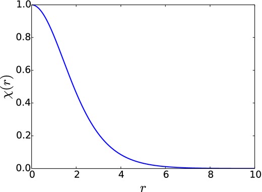
Zero-node soliton profile χ(r) found by solving the BVP system in equation (A25).

Open in new tab Download slide

Figure A2.

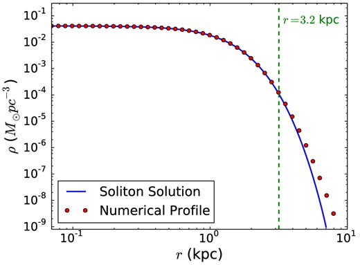
In blue is depicted the density profile obtained from the zero-node soliton solution, scaled to typical dwarf galaxy parameters, while in red we show the fit of equation (A52). This provides a good fit to the BVP solution up to radius r ≈ 3.2 kpc.

Open in new tab Download slide

A6 Fitting the soliton density profile

We fit the ground state soliton density profile, |$\tilde{\rho }=f(\alpha r)$|⁠, for different functional forms. We begin with the form used by Schive et al. (2014a):

\begin{equation} f(\alpha r) = \frac{1}{(1+\alpha ^2 r^2)^8}. \end{equation}

(A47)

In Schive et al. (2014a,b) the soliton–NFW transition generally occurs for ρ ∼ 0.01ρ(0). Therefore we perform a best fit for the value of α with r chosen so that |$\tilde{\rho }\in [0.01,1]$|⁠. For this range of r we find α = 0.230. The fit is shown in Fig. A2.

The fit equation (A48) has a number of advantages. It gives an analytic expression for the mass integrated out to any radius. Assuming this form for the density, one can also find an analytic solution for the Newtonian potential V(r) from the Poisson equation, and the combined solution can be shown to give an accurate solution to the full SP system. Allowing the exponents in the fit to vary can improve the fit slightly at large radius, but loses these computational advantages. In our complete profile the large radius region occurs after the transition to NFW and improving the soliton fit here does not have any effect.

We also investigate a Gaussian fit:

\begin{equation} f(\alpha r)= \mathrm{exp}\left[-\frac{r^2}{2\sigma ^2}\right], \end{equation}

(A48)

and find |$\sigma = \alpha ^{-1}/\sqrt{2}= 1.22$|⁠. This form of the density profile also gives analytic results for the soliton mass, and of slightly simpler form than for the polynomial fit. However, we find that the Gaussian profile always gives a worse fit than the polynomial, and consider it no further.

Schive et al. (2014a) solved the system of ODEs in equation (3) using the shooting method and the boundary conditions of Guzmán & Ureña-López (2006):

\begin{eqnarray} \phi (0) &=& \mathrm{\partial} _r \phi (0) = 0, \end{eqnarray}

(A49)

\begin{eqnarray} \phi (r \rightarrow \infty ) &=& 0, \end{eqnarray}

(A50)

\begin{eqnarray} V(\infty ) &=& 0. \end{eqnarray}

(A51)

Schive et al. (2014a)'s fit for the soliton density profile is

\begin{equation} \rho _{\rm sol} (r) \simeq \frac{1.9 \, (m_B/10^{-23}\, \mathrm{eV})^{-2} (r_{1/2}/\mathrm{kpc})^{-4}}{[1+9.1 \times 10^{-2} (r/r_{1/2})^2]^8}\, {\rm M}_{{\odot }} \, \mathrm{pc}^{-3} , \end{equation}

(A52)

where they define r_1/2 such that ρ_sol(r_1/2) = ρ_sol(0)/2. This fixes the factor 9.1 × 10⁻² and the value of α is found by normalizing the central density. Restoring units using the scaling symmetry, as outlined in Section 2.2, shows good agreement between this fit and ours.

APPENDIX B: A NOTE ON SOLITONS

We have considered spherically symmetric soliton solutions to equations (1). In this model, the non-linearity necessary to support solitons comes purely from gravity. Real fields such as axions form a class of solitons known as oscillons, which, being unprotected by a charge, are technically pseudo-solitons. Oscillatons are oscillons including self-gravity. The solutions we study evade Derrik's theorem that otherwise forbids solitons in three spatial dimensions because they are time dependent and include self-gravity. Scalar field solitons known as boson stars are formed for complex fields, where stability is guaranteed by the charge. For more discussion of solitons, oscillons, and boson stars in various contexts, see e.g. Ruffini & Bonazzola (1969), Liddle & Madsen (1992), Liebling & Palenzuela (2012), Amin et al. (2012), Amin (2013) and Lozanov & Amin (2014).

We considered the ground state solitons. An isolated system relaxes to the ground state via the emission of scalar waves to infinity, a process of ‘gravitational cooling’ (Seidel & Suen 1994; Guzmán & Ureña-López 2006). Stable solutions are the non-linear density profiles that form the end-point of spherical collapse in axion DM haloes below the threshold for black hole formation. These solutions are pressure supported. By analogy to stars, this justifies the use of spherical symmetry, as we expect the relaxation time for non-spherical perturbations to be on the same time-scale as the relaxation time to the ground state. The simulations of Schive et al. (2014a) show that these ground state solitons form and are stable on cosmological time-scales.

During cosmological structure formation, such ground state solutions will only be found locally if the relaxation time is shorter than the age of the universe, with the relaxation time being shorter for denser objects. These solitons will possess a characteristic size related to their formation time. CDM-like structure will form on larger scales due to the Jeans instability (Khlopov et al. 1985). Furthermore, in bound states such as haloes, scalar waves may not escape to infinity and may contribute to the outer parts of a halo. Detailed questions about the non-linear dynamics can only be solved by simulation and will be the subject of future work.

Download all slides

Month:	Total Views:
December 2016	1
January 2017	2
February 2017	9
March 2017	6
April 2017	12
May 2017	8
June 2017	19
July 2017	4
August 2017	4
September 2017	2
October 2017	7
November 2017	4
December 2017	1
January 2018	3
February 2018	2
March 2018	12
April 2018	6
May 2018	5
June 2018	3
July 2018	8
August 2018	21
September 2018	12
October 2018	3
November 2018	21
December 2018	20
January 2019	27
February 2019	29
March 2019	61
April 2019	43
May 2019	48
June 2019	16
July 2019	27
August 2019	22
September 2019	31
October 2019	33
November 2019	37
December 2019	50
January 2020	50
February 2020	71
March 2020	59
April 2020	48
May 2020	58
June 2020	51
July 2020	57
August 2020	46
September 2020	44
October 2020	49
November 2020	44
December 2020	40
January 2021	40
February 2021	47
March 2021	65
April 2021	32
May 2021	33
June 2021	46
July 2021	42
August 2021	45
September 2021	40
October 2021	43
November 2021	33
December 2021	34
January 2022	52
February 2022	47
March 2022	84
April 2022	68
May 2022	44
June 2022	41
July 2022	51
August 2022	49
September 2022	65
October 2022	53
November 2022	55
December 2022	57
January 2023	42
February 2023	49
March 2023	56
April 2023	48
May 2023	35
June 2023	48
July 2023	29
August 2023	43
September 2023	32
October 2023	33
November 2023	56
December 2023	23
January 2024	43
February 2024	42
March 2024	74
April 2024	83
May 2024	56
June 2024	62
July 2024	38
August 2024	44
September 2024	37
October 2024	45
November 2024	60
December 2024	39
January 2025	53
February 2025	44
March 2025	64
April 2025	56
May 2025	33

Article Contents

Axion dark matter, solitons and the cusp–core problem

Abstract

1 INTRODUCTION

2 SOLITON CORES FOR SCALAR DM

2.1 Schrödinger–Poisson system and ground state solitons

2.2 Soliton core radius

3 AXION HALO DENSITY PROFILES AND DWARF GALAXY CORES

3.1 Defining the density profile

3.2 Fitting to Fornax and Sculptor

4 DISCUSSION AND CONCLUSIONS

REFERENCES

APPENDIX A: THE SCHRÖDINGER–POISSON SYSTEM

A1 Derivation

A2 Dimensionless variables

A3 Scaling relations

A4 Power-law solutions

A5 Numerical solutions

A5.1 Boundary conditions

A5.2 Solution of the boundary value problem

A6 Fitting the soliton density profile

APPENDIX B: A NOTE ON SOLITONS

Citations

Views

Altmetric

Email alerts

Astrophysics Data System

Citing articles via

Latest

Most Read

Most Cited

Article Contents

Axion dark matter, solitons and the cusp–core problem Free

Abstract

1 INTRODUCTION

2 SOLITON CORES FOR SCALAR DM

2.1 Schrödinger–Poisson system and ground state solitons

2.2 Soliton core radius

3 AXION HALO DENSITY PROFILES AND DWARF GALAXY CORES

3.1 Defining the density profile

3.2 Fitting to Fornax and Sculptor

4 DISCUSSION AND CONCLUSIONS

REFERENCES

APPENDIX A: THE SCHRÖDINGER–POISSON SYSTEM

A1 Derivation

A2 Dimensionless variables

A3 Scaling relations

A4 Power-law solutions

A5 Numerical solutions

A5.1 Boundary conditions

A5.2 Solution of the boundary value problem

A6 Fitting the soliton density profile

APPENDIX B: A NOTE ON SOLITONS

Citations

Views

Altmetric

Email alerts

Astrophysics Data System

Citing articles via

Latest

Most Read

Most Cited

This Feature Is Available To Subscribers Only

Axion dark matter, solitons and the cusp–core problem