


Abstract
The m–z relation for Type Ia supernovae is one of the key pieces of evidence supporting the cosmological ‘concordance model’ with λ0 ≈ 0.7 and Ω0 ≈ 0.3. However, it is well known that the m–z relation depends not only on λ0 and Ω0 (with H0 as a scale factor) but also on the density of matter along the line of sight, which is not necessarily the same as the large-scale density. I investigate to what extent the measurement of λ0 and Ω0 depends on this density when it is characterized by the parameter η (0 ≤ η ≤ 1), which describes the ratio of density along the line of sight to the overall density. I also discuss what constraints can be placed on η, both with and without constraints on λ0 and Ω0 in addition to those from the m–z relation for Type Ia supernovae.
1 INTRODUCTION
In the last 15 years or so, cosmological observations have improved greatly and it also appears that the values are converging on their true values.1 This allows us to answer such questions (provided, of course, that ‘standard assumptions’ hold) as whether the Universe will expand for ever (yes), how old it is, whether it is accelerating now (yes), when it started accelerating, etc. (With the assumption of a simple topology, the Universe is finite if λ0 + Ω0 > 1, but since observations indicate that this value is very close to 1, we cannot yet answer this question.) Among the most important of these observations are those by the Supernova Cosmology Project (e.g. Goobar & Perlmutter 1995; Perlmutter et al. 1995, 1998, 1999; Amanullah et al. 2010; Suzuki et al. 2012) and the High-z Supernova Search team (e.g. Garnavich et al. 1998; Riess et al. 1998; Riess et al. 2000) (see also the reviews by Riess 2000, Leibundgut 2001, 2008, and Goobar & Leibundgut 2001) which provide joint constraints on λ0 and Ω0. Combined with other observations (e.g. Komatsu et al. 2011; Planck Collaboration XVI, 2014), these lead to quite well constrained values for the cosmological parameters (e.g. fig. 5 in Suzuki et al. 2012). Although the supernova data alone allow a relatively wide range of significantly different other models, it is interesting that the best-fitting values obtained from these observations using the current data are quite close to the much better constrained values using combinations of several observations without the supernova data, at least under the assumptions with which the former were calculated. However, since the m–z relation depends not only on λ0 and Ω0 (with H0 as a scale factor) but also on the distribution of matter along and near the line of sight, the dependence of conclusions drawn from the m–z relation for Type Ia supernovae on this matter distribution should be investigated. Alternatively, these observations can perhaps tell us something about this distribution.
The plan of this paper is as follows. Section 2 sketches the basic theory used in this paper. In Section 3, I briefly review previous investigations of the influence of a locally inhomogeneous universe on the m–z relation. Section 4 describes the calculations done and discusses the results. Summary, conclusions and outlook are presented in Section 5.
2 BASIC THEORY
Kayser, Helbig & Schramm (1997, hereafter KHS) developed a general and practical method for calculating cosmological distances in the case of a locally inhomogeneous universe. See KHS for details (and for a description of the notation, which is followed here); here I repeat only the most important points for the purpose of this paper.
This change, compared to the perfectly homogeneous case, is essentially a negative gravitational-lensing effect. In a conventional gravitational-lensing scenario, if the density at a given redshift between two light rays is higher than the overall density (the corresponding overdensity being ‘the lens’), then there will be more convergence than in the case where the two densities are the same. In the case of light propagating between clumps, as described above, the situation is reversed, and the density between the light rays defining the distance-related angle is less than the overall density. This means that there is (negative) Ricci focusing (and no Weyl focusing), making objects appear fainter than they would be in the completely homogeneous case. Of course, this is only a rough model, but can be expected to be more realistic than the completely homogeneous case and to determine not just the sign of the difference but also give at least an estimate of its strength.
Obviously, one cannot have η < 0. However, it does not make sense to have η > 1 either. While it is certainly possible that the average density inside the beam could be greater than the global density, such cases are either unrealistic or not useful. The limiting case where the density in the beam is greater than the global density by a constant factor at every redshift is unrealistic because this would imply the existence of overdense regions with an extreme length-to-width ratio which are aligned between us and the source, which is incompatible with homogeneity and isotropy on large scales and would also put us in a special position. The other limiting case where a single compact object increases the density in the beam to above the global density is certainly possible, but observationally would show up as a gravitational-lens effect and should be analysed as such (perhaps by adopting η ≈ 0 for the distance calculation and explicitly calculating the amplification). Of course, cases between these two extremes are possible, but it is clear that η must be between 0 and 1 if it is used as an additional parameter in the manner described by KHS; lines of sight which, due to fluctuations, are slightly denser than the overall density are certainly possible, but are not usefully parametrized by η in the style of KHS. (But see Lima, Busti & Santos 2014 for a toy model with an interesting extension of the η concept.) Note that η does not have to be constant as a function of redshift, and the code described in KHS supports an arbitrary dependence of η on z. Also, it could be different for different lines of sight. It was pointed out by Weinberg (1976) that η must be 1 when averaged over all lines of sight (allowing for the moment higher-than-global densities to be parametrized by η > 1), which follows from flux conservation. However, in practice lines of sight will probably avoid concentrations of matter, due to selection effects or design: distant objects will be more difficult to observed if there is luminous matter along the line of sight or if there is absorbing matter along the line of sight.3 If these selection effects do not exist, and if the sample is large enough, then the ‘Safety in Numbers’ effect (Holz & Linder 2005) allows one to effectively assume η = 1, with inhomogeneity merely increasing the dispersion, roughly linearly with redshift. However, Clarkson et al. (2012) point out that most narrow-beam lines of sight are significantly underdense, even for beams much thicker than those considered in this paper. (On the other hand, they also point out that this does not necessarily lead to a reduction in brightness if one drops the assumption that inhomogeneities can be modelled as perturbations on a uniformly expanding background, a point also emphasized by Bolejko & Ferreira 2012; see also Bagheri & Schwarz 2014.)
The situation discussed above corresponds to the situation where the beam contains a density η times the global density at a given redshift and outside the beam the density is equal to the global density. In practice, this means that a fraction η of the mass in the universe is smoothly distributed and a fraction 1 − η is contained in clumps outside the beam. Of course, ‘smoothly’ depends on the size of the beam; for example, small objects are part of the ‘smooth’ component, not only in the limiting case where the smooth component consists of free elementary particles. The important point is that their angular size is small compared to that of the beam. η is thus also a function of angle: the larger the angle, the more representative is the matter within the beam, so that η approaches 1 for large enough angles. Since the beams of supernovae at cosmological distances are extremely thin objects (the thinnest objects ever studied by science), evidence for η < 1 should be most obvious in the m–z relation for Type Ia supernovae.
A given value of η along a given line of sight does not imply that this value does not change along the line of sight, although that is of course a possibility, but rather that the influence on angle-dependent distances can be described by an effective value of η which is some appropriate average of a value which varies along the line of sight. This means that it is possible for the density along the line of sight to be larger than the global density at some points, but this is not in contrast with the claim above that η > 1 is not useful as long as the effective value ηeff ≤ 1. Another complication is that essentially all lines of sight to supernovae will have a density higher than the globally average cosmological density due to the overdensities associated with the Milky Way and with the supernova host galaxy (and corresponding clusters).4 However, since the absolute magnitudes of supernovae are not known from first principles, but rather calibrated from observations, this effect is, to a first approximation, unobservable, since it is essentially a renormalization of the absolute magnitude. Even if this extra matter associated with the galaxies at the ends of the beam would increase the density inside the beam to larger than the global density, it is not useful to think of this as η > 1, since I want to compare the standard assumption (completely homogeneous Universe, at least as far as light propagation is concerned) with that of a more realistic distribution. The point of comparison, the m–z-relation for a homogeneous Universe, also contains extra matter at each end of the beam, and hence extra convergence. As far as I know, no-one has ever taken this into account and it is not necessary if one is interested only in the differences. (This would have to be taken into account, though, if the absolute magnitude of objects at cosmological distances were known independently of observation.)
Although the term ‘dark matter’ suggests something opaque, the defining characteristic is lack of interaction with electromagnetic radiation. Thus, not only does dark matter not glow, it is also transparent. It is thus irrelevant whether dark-matter objects within the beam significantly cover a source as seen by an observer. (Of course, when comparing observed to calculated brightness, one must correct for extinction due to ‘conventional’ matter – it can also be dark in the sense that it does not radiate, but it is not transparent.) Here, I am using the term ‘dark matter’ to refer to the ‘missing matter’, i.e. that responsible for the difference between the density due to baryonic matter (other non-baryonic but known particles (neutrinos) do not increase this significantly) and the global density of the Universe, as measured on large scales. Of course, non-radiating baryonic matter does exist, but we know from constraints from big-bang nucleosynthesis that this cannot be a significant fraction of the missing matter. This reflects current usage, e.g. the ‘DM’ in ‘ΛCDM’, and is more convenient than ‘not yet identified non-baryonic matter’.
Since we know that the Universe is not exactly homogeneous and isotropic, η ≠ 1 is the most obvious departure from the simplest cosmological model (the Einstein–de Sitter model with λ0 = 0, Ω0 = 1, and η = 1, although the last item is often not stated explicitly), but there is not much literature on this topic. (There are, though, several recent papers investigating whether ‘dark energy’ could be something other than the traditional cosmological constant, e.g. whether the equation of state w differs from −1, whether it changes with time etc, even though there are no observations which indicate this. Of course, that does not mean that one should not look.)
If η is allowed to vary from one line of sight to another, one could regard this as an additional contribution to the uncertainty in the distance modulus, much the same as the uncertainty in the absolute magnitude. Theoretically, fitting the observations for a constant value of η would result in a worse fit for such cases if this additional uncertainty is ignored or in a larger allowed region of parameter space if it is included in the error budget. With some assumptions, one could try to take this additional dispersion into account and/or correct for it; see e.g. Amanullah, Mörtsell & Goobar (2003), Gunnarsson et al. (2006), Jönsson et al. (2006), Jönsson, Mörtsell & Sollerman (2009). In practice, with a large number of objects and only a few variables, the difference in goodness of fit is well within the expected range of values for the case in which η is the same along all lines of sight. Alternatively, with current data it is also a relatively small contribution to the error budget. Thus, if observations suggest 0 < η < 1, it would be unclear if this is evidence for the corresponding value of the global value of η or whether this is a compromise between lines of sight with lower and higher values. However, if observations indicate η = 0 or η = 1, then this would be evidence for the corresponding global value, because these are the extreme values of η and cannot result from averaging.
Of course, more complicated models are possible. In this paper, I consider only models in which η is a constant function of redshift and the same along all lines of sight5; also, in all cases but one, it is independent of the other cosmological parameters. The variation between these models, however, is certainly larger than the realistic range of the possible influence of η on the m–z relation for Type Ia supernovae.
3 BRIEF HISTORY
The effects of a locally inhomogeneous universe on quantities important for observational cosmology were first investigated in a series of papers by Zeldovich (1964), Dashevskii & Zeldovich (1965), and Dashevskii & Slysh (1966). Dyer & Roeder (1972) discussed the special case of λ0 = 0 but with Ω0 as a free parameter for η = 0 (where there is an analytic solution) and for general η values (Dyer & Roeder 1973). As a result, the distance for η = 0 is sometimes referred to as the Dyer–Roeder distance. KHS presented a second-order differential equation and numerical implementation valid for the general case (−∞ < λ0 < ∞, 0 ≤ Ω0 ≤ ∞, 0 ≤ η ≤ 1). Kantowski and collaborators (Kantowski 1969, 1998, 2003; Kantowski, Vaughan & Branch 1995; Kantowski, Kao & Thomas 2000; Kantowski & Thomas 2001) have stressed the importance of η for the interpretation of the m–z relation for Type Ia supernovae and have provided numerical implementations using elliptic integrals for the special values of η of 0, |$\frac{2}{3}$|, and 1. Perlmutter et al. (1999) considered the effect of η ≠ 1 on their results (see their fig. 8) and concluded that, at least in the ‘interesting’ region of the λ0–Ω0 parameter space, it had a negligible effect (see also Jönsson et al. 2006). The reason for the current paper is that, with the larger number of supernovae now available, this is no longer the case. Further investigation has often been motivated by the m–z relation for Type Ia supernovae (e.g. Goliath & Mörtsell 2000; Mörtsell, Goobar & Bergström 2001). It has also been investigated, via comparison with explicit ray-tracing through mass distributions derived from simulations or observations, whether η is a useful parametrization for local inhomogeneity (e.g. Bergström et al. 2000; Mörtsell 2002) (and the conclusion is that it is a useful approximation, at least for cosmological models which are otherwise realistic).
There seem to be three schools with respect to the attitude taken to the possible influence of inhomogeneities on cosmological parameters derived from the m–z relation for Type Ia supernovae. One school ignores it completely, assuming a completely homogeneous Universe as far as the calculation of the luminosity distance is concerned (e.g. Riess et al. 1998), or provides some limited justification for not considering it further (e.g. Betoule et al. 2014). Another school emphasizes that the problem is not completely understood, the amount of uncertainty is unknown, and even the sign of some effects is unclear (e.g. Clarkson et al. 2012). A third school uses some approximation to at least get an idea of the size of possible effects (e.g. Mörtsell et al. 2001). (While Perlmutter et al. 1999 did consider the possible influence of η, hence belonging to the third school, at least at that time, with their data then it was not a significant source of uncertainty in their main result. One purpose of this paper is to show that this is no longer the case.)
4 CALCULATIONS, RESULTS AND DISCUSSION
I have used the publicly available ‘Union2.1’ sample of supernova data (Suzuki et al. 2012) and calculated χ2 and the associated probability following Amanullah et al. (2010) on regularly-spaced grids of various extents and resolutions in the λ0–Ω0–η parameter space. This assumes, of course, that η is a free parameter on the same footing as λ0 and Ω0. My goal is not to obtain the ‘best’ cosmological parameters, not even the ‘best’ ones from the supernova data alone. Rather, it is to investigate the influence of η ≠ 1 on the interpretation of the m–z relation for Type Ia supernovae. I have thus intentionally made the supernova data as precise as possible, by using only the statistical uncertainties (i.e. column 4 in the publicly available data file) and fixing H0 at 70 km s−1 Mpc−1, which implies M = −19.318 276 1161. Thus, all increase in the allowed region of parameter space (at a given confidence level) is due only to the influence of η.6
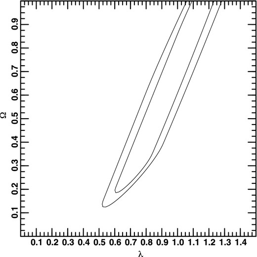
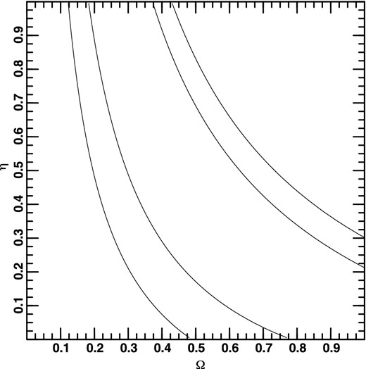
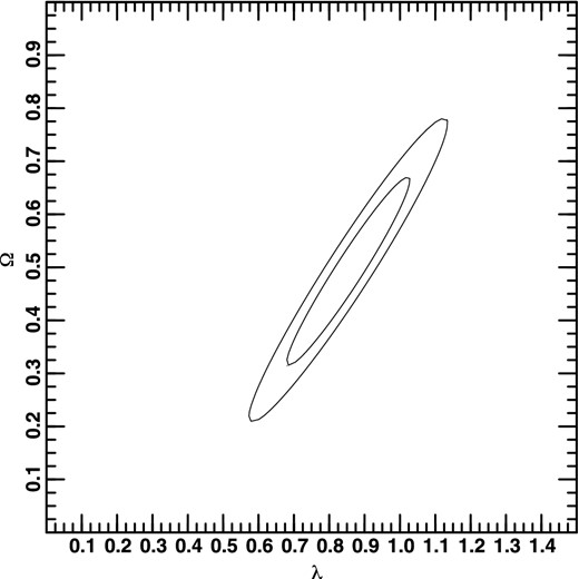
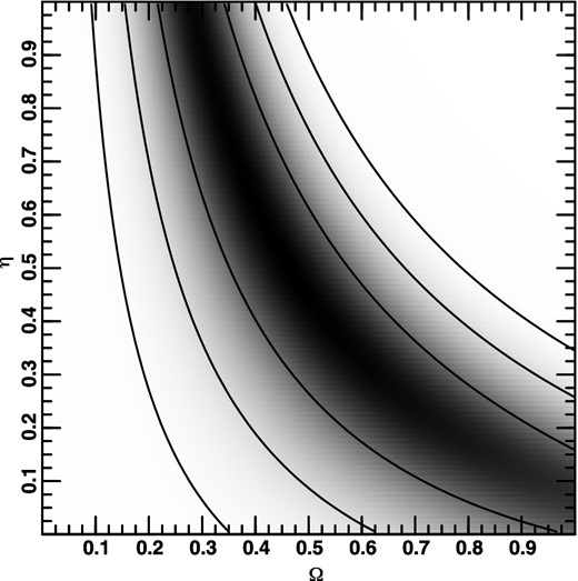
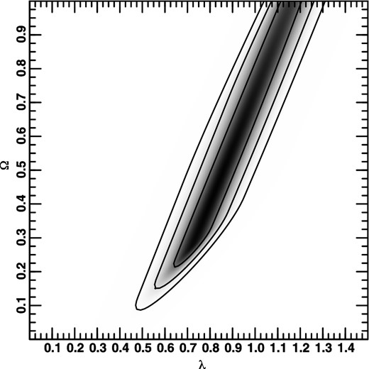
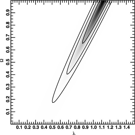
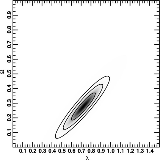
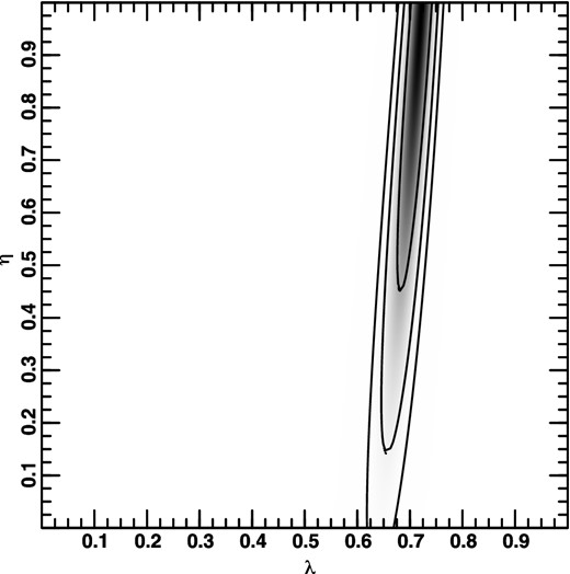
All contours in two (three) dimensions have been calculated as the smallest-area closed curve (smallest-volume closed surface) which encloses the corresponding fraction of the probability. I have used the standard values 0.683, 0.954, and 0.997; these correspond to 1σ, 2σ, and 3σ in the Gaussian case. However, I have made no assumption about Gaussianity, since I have calculated the contours explicitly, rather than plotting them at the corresponding fraction of the peak likelihood under the Gaussian assumption. For all plots, the area outside of the plot has been assigned a probability of zero. Otherwise, no priors other than those explicitly stated have been used. In particular, no prior information on the values of the cosmological parameters from other tests have been used; what I show, depends on the supernova data only. Figs 1, 2, and 3 show projections of the three-dimensional contours along one axis on to the plane spanned by the other two axes for the smaller, higher-resolution grid. It can be seen that the combination of λ0 and Ω0 is well constrained, as are both individually, while η is hardly constrained at all. Note also that λ0 and Ω0 are less constrained for lower values of η. (The contours at 0.954 and 0.997 cannot be distinguished in these plots.) The relatively sharp bend in the lower-right contours in Figs 1 and 2 is due to the fact that I have assigned a probability of 0 to models which have no big bang (see the discussion of figs 1 and 2 in Helbig 2012 and references therein for an explanation).
Projection of three-dimensional probability distribution along the η-axis.
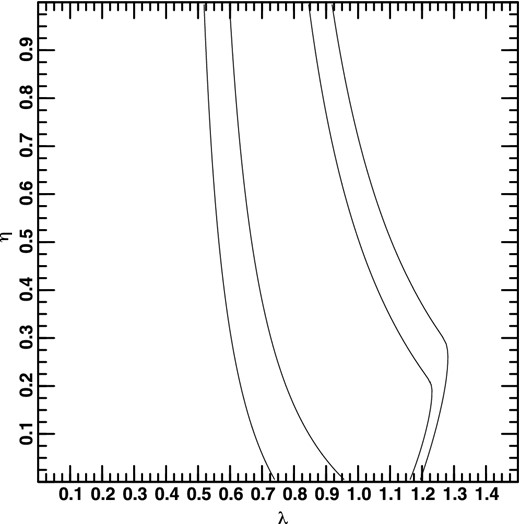
Projection of three-dimensional probability distribution along the Ω0-axis.
Projection of three-dimensional probability distribution along the λ0-axis.
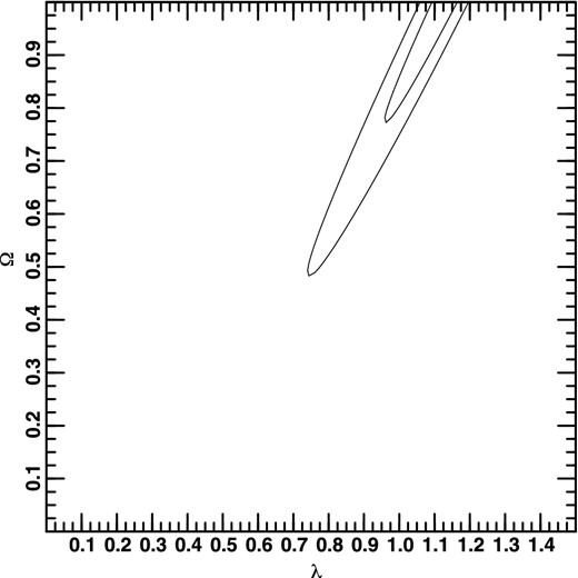
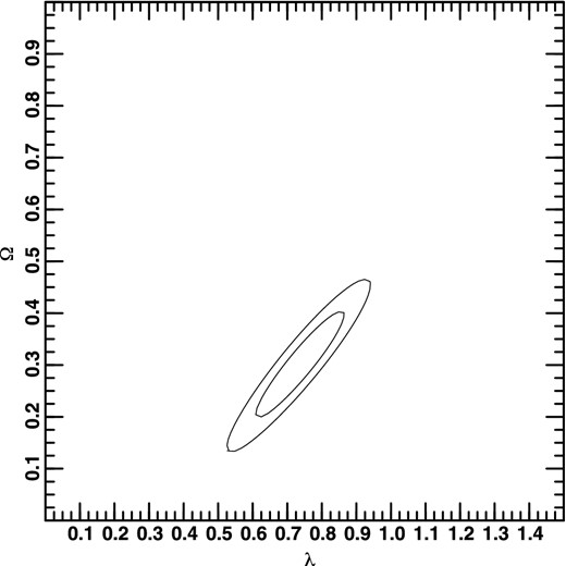
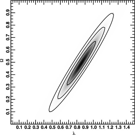
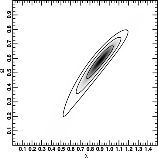
Another way of visualizing these three-dimensional contours is to make cuts through them for a fixed value of one of the parameters. Figs 4, 5, and 6 show cuts for η = 0.005, 0.455, 0.955. The contours become smaller and move to lower values of λ0 and Ω0 as η becomes larger. (Again, the contours at 0.954 and 0.997 cannot be distinguished in these plots.) Fig. 6 is quite similar to standard presentations of the supernova constraints (e.g. Suzuki et al. 2012), but keep in mind that these contours are a cut through the three-dimensional contours for a fixed value of η, not two-dimensional contours. If η is substantially less than 1, then not only is the allowed region much larger, but the ‘concordance model’ with λ0 ≈ 0.7 and Ω0 ≈ 0.3 is ruled out. Qualitatively, this behaviour is easy to understand: there is some degeneracy between η and λ0 + Ω0 since both increase the amount of focusing in the beam, the former because there is more matter in the beam and the latter because of the increase in the global curvature, which is essentially λ0 + Ω0. When there is essentially no matter in the beam, then the value of Ω0 is less important and hence not as well constrained. This means that λ0 + Ω0 can be realized via a larger range of each parameter, making the allowed region larger. The middle value of η is that of the global maximum probability. (Since λ0 and Ω0 are better constrained, the corresponding plots for fixed values of these parameters, not shown here, are less interesting.)
Cut through the three-dimensional probability distribution perpendicular to the η-axis for η = 0.005.
Cut through the three-dimensional probability distribution perpendicular to the η-axis for η = 0.455.
Cut through the three-dimensional probability distribution perpendicular to the η-axis for η = 0.955.
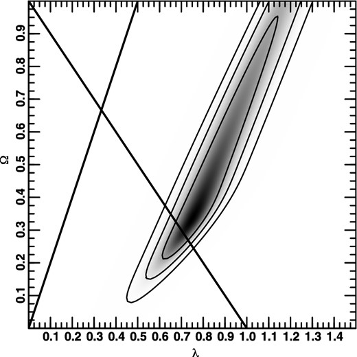
Two-dimensional probability distribution obtained by marginalizing over η.
The ‘standard procedure’ for reducing the number of parameters shown in a plot is to marginalize over the less interesting or ‘nuisance’ parameters. This is shown in Figs 7, 8, and 9. Here, and in similar figures below, the grey-scale corresponds to the probability.7 These are qualitatively similar to the projections. Fig. 7 also contains two straight lines corresponding to a flat universe with λ0 + Ω0 = 1 (negative slope) and zero acceleration (|$q_{0} = \frac{\Omega _{0}}{2} - \lambda _{0}= 0$|) (positive slope). Note that a flat universe is compatible with the data but not required by them; in fact, the degeneracy in the constraints is almost perpendicular to the flat-universe line. In this particular plot, the degeneracy corresponds roughly to q0 ≈ −0.6; in many of the other plots, the degeneracy in the λ0–Ω0 plane is closer to a constant value of Ω0 − λ0 than to a constant value of |$q_{0} = \frac{\Omega _{0}}{2} - \lambda _{0}$|. (q0 was important historically since the departure from the linearity of the m–z relation at low redshift is proportional to q0; nowadays quoting a value for q0 derived from the m–z relation for higher-redshift objects is neither necessary nor sufficient nor, in general, meaningful.)
Another approach is to maximize the ‘nuisance’ parameter, i.e. for a given point in the plane of the plot, find the value of the third parameter which maximizes the probability. This is shown in Fig. 10. (For these data, such plots are very similar to those where the third parameter has been marginalized over, so only this one example is shown.)
Most discussion of the m–z relation for Type Ia supernovae has concentrated not on contours of more than two dimensions, nor on some reduction (projection, cut, marginalization, maximization) of these higher-dimensional contours to two dimensions, but rather on two-dimensional contours, i.e. with a δ-function prior on the nuisance parameters. Almost always, of course, the (often implicitly assumed) prior is η = 1. For comparison, in Figs 11, 12, and 13 I show constraints in the λ0–Ω0 plane for fixed values of η, namely 0, 0.455 (the value at the maximum of the three-dimensional probability distribution) and 1. The last should be compared with e.g. fig. 11 in Kowalski et al. (2008), but keep in mind that, as mentioned above, I have fixed H0 and use only the statistical uncertainties. (See also figs 1a and 5a in Amanullah et al. 2003.) Thus, Fig. 13 has slightly smaller contours than similar plots elsewhere in the literature. Again, this is intentional so that any deviations from this fiducial plot (larger and/or shifted contours) are due solely to the influence of η.
Of course, little significance should be placed on variations in the probability within the innermost contour, since the probability that the point representing the true values of λ0 and Ω0 is only about twice as likely to lie inside this contour than outside it. Nevertheless, it is remarkable that the maximum of the probability in Fig. 13 is at λ0 = 0.721 0938 and Ω0 = 0.277 3438, i.e. at the values of the concordance model (within the small uncertainties; these are much smaller than even the 68.3 per cent contour in Fig. 13).8 Note that when fewer supernova data were available, the best-fitting value was at much higher values of λ0 and Ω0; see e.g. fig. 1 in Helbig (1999). (As mentioned above, the best-fitting value is often not visible in modern versions of such plots, though of course it can be easily found in the data used to make the plots.) If the best-fitting value remains the same when significantly more supernova data are available, then very probably the true value will have been converged upon, even though the range of values allowed, even at the 68.3 per cent level, would include values well outside what is acceptable when other cosmological constraints are considered (i.e. joint constraints from several cosmological tests). Normally, when more data are available one expects the new best-fitting value to be consistent with, but different from, the old best-fitting value, as has been the case with the supernova data up until now. However, looking towards the future, I don't expect the best-fitting values for λ0 and Ω0 to change significantly, but do expect the constraints from the supernova data to improve, which appears somewhat puzzling. A possible explanation for this is that the statistical errors in the supernova data have been overestimated. Note, however, that the best-fitting values for the supernova data correspond to the concordance model only if one assumes η ≈ 1. For η = 0.455, the concordance model lies very near the 95.4 per cent contour, and for η = 0 it is even outside the 99.7 per cent contour. The plots above illustrate that it is not possible to appreciably constrain η from the supernova data alone. However, the fact that the supernova data suggest the concordance model only for high values of η could be seen as evidence that η ≈ 1.
A similar result is shown in Fig. 14, where a flat universe (λ0 + Ω0 = 1) has been assumed. As in the other plots, λ0 is reasonably well constrained, while η is quite weakly constrained. (In this case, since Ω0 = 1 − λ0, Ω0 is just as well constrained; in general, Ω0 is less well constrained than λ0.) However, note that the best-fitting value is for η = 1 and λ0 ≈ 0.72; in other words, again the best fit is for the concordance model with η = 1. (This plot also shows the importance of plotting the probability and not just a few contours.)
To illustrate the change in the effect of η now that more supernova data are available, Fig. 15 shows the constraints where η is a function of Ω0, namely η = 0 for Ω0 ≤ 0.25 and 1 − 0.25 for Ω0 ≥ 0.25. This should be compared with fig. 8 in Perlmutter et al. (1999). In that figure, the red contours were calculated in the same way as those in Fig. 15. In the same figure, the green contours were calculated in the same way as in Fig. 11. The comparison illustrates vividly the fact that the effect of η can no longer be neglected. While Perlmutter et al. (1999) concluded that, at least in the interesting part of parameter space, the constraints on λ0 and Ω0 from the supernova data did not depend heavily on the assumed value of η, this is definitely no longer the case.
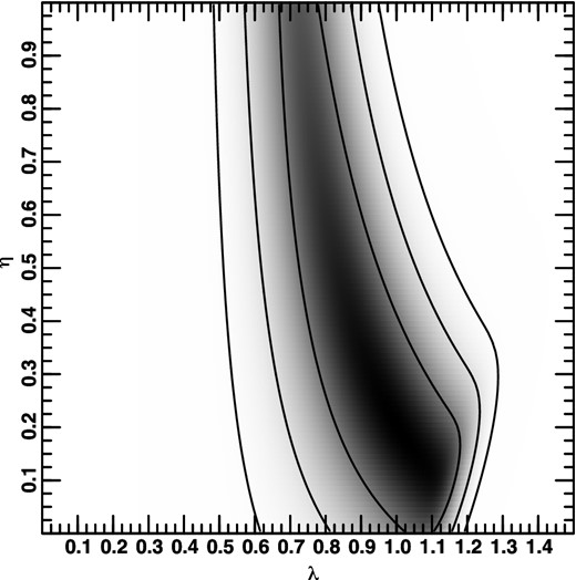
Two-dimensional probability distribution obtained by marginalizing over Ω0.
Two-dimensional probability distribution obtained by marginalizing over λ0.
Two-dimensional probability distribution obtained by maximizing η.
Two-dimensional probability distribution for η = 0.
Two-dimensional probability distribution for η = 0.455.
Two-dimensional probability distribution for η = 1.
Two-dimensional probability distribution for k = 0.
Two-dimensional probability distribution with η = f(Ω0).
One-dimensional probability distribution for the concordance model.
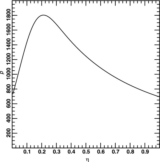
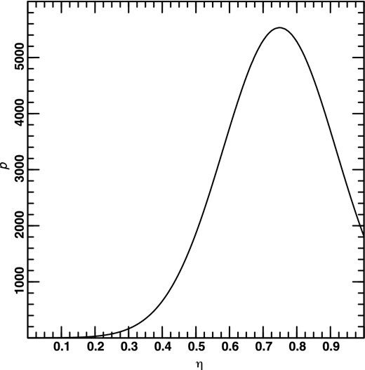
One-dimensional probability distribution after marginalizing over λ0 and Ω0.
(This can be contrasted with Fig. 17 which shows the value of η preferred by the supernova data alone; λ0 and Ω0 have been marginalized over.) While η = 1 is not ruled out at high confidence, lower values of η are ruled out at a high level of statistical significance.9 This suggests that η is relatively large, even though the beams of supernovae at cosmological distances are extremely thin and this cosmological test should suggest a value of η lower than that of any other cosmological test known today. One would not expect to obtain η = 1 since some matter is associated with galaxies which are outside the beam; such mass contributes about 0.1 to Ω0. Fig. 16 thus suggests that dark matter is distributed much more smoothly than galaxies. While the beam of a supernova at cosmological distance is almost a fair sample of the universe, it is an even fairer sample of dark matter. Dark matter is thus not significantly clumped at the scale of a supernova beam.
5 SUMMARY, CONCLUSIONS, AND OUTLOOK
The following conclusions were more or less expected.
Constraints on λ0 and Ω0 are weaker if η is not constrained.
The concordance model is reasonably probable.
There is a degeneracy between η and the amount of spatial curvature (λ0 + Ω0).
λ0 is constrained best, then Ω0, then η.
The following conclusion was neither expected nor surprising.
Even when η is allowed to be a free parameter, the m–z relation for Type Ia supernovae is not compatible with |$q_{0} = \frac{\Omega _{0}}{2} - \lambda _{0}\ge 0$|, and thus implies that the universe is currently accelerating.10 (Even though the m–z relation for Type Ia supernovae is one of the key pieces of evidence supporting the cosmological ‘concordance model’ with λ0 ≈ 0.7 and Ω0 ≈ 0.3, it is not an essential piece in the sense that combinations of other tests still result in the same concordance model. Nevertheless, it is still an important piece of evidence in favour of the concordance model since it is the only single test which, without additional assumptions, implies q0 < 0, i.e. a universe which is currently accelerating.)
The following conclusions are somewhat surprising.
The overall (in the three-dimensional parameter space) best-fitting values for λ0 and Ω0 are ruled out by other cosmological tests. Probably, this best-fitting point is the result of overfitting: its probability is not significantly higher than elsewhere and the allowed region is quite large.
If one assumesk = 0, then the best fit is very close to the concordance model and has η = 1.
If one assumes η = 1, then the best fit is very close to the concordance model.
If one assumes the concordance model, then one can probably rule out low values of η, even though the relevant scale is extremely small, which implies that dark matter is much less clustered than galaxies are.
We cannot rule out η = 1, and there is some tentative evidence for it.
To summarize, allowing η, which is otherwise only weakly constrained, as a free parameter significantly alters both the best fit in the λ0–Ω0 plane and the allowed region of this plane. The concordance model is, however, still allowed. There are hints that η ≈ 1, though these are not statistically significant when examined in the three- or two-dimensional parameter space. On the other hand, if one assumes the concordance values for λ0 and Ω0, low values of η can probably be ruled out, which is not obvious considering the very small scales involved; this implies that dark matter is very homogeneously distributed.
One might have thought that the increase in the number of data points since Perlmutter et al. (1999) would allow some sort of useful constraint to be placed on η from the supernova data without further assumptions. This is not the case. Even worse, if η is allowed to vary, then the conclusions about the cosmological model derived from the m–z relation for Type Ia supernovae are not as robust. However, as discussed in Section 1, current constraints from combinations of cosmological tests without using the supernova data determine the ‘concordance model’ with λ0 ≈ 0.7 and Ω0 ≈ 0.3 to rather high precision. It is thus perhaps more interesting to assume the concordance model and use the supernova data to constrain η, especially since η is otherwise difficult to measure. Indeed, as shown in Fig. 16, current data already provide interesting constraints. It is also extremely interesting that the supernova data have the best-fitting values for λ0 und Ω0 corresponding to those of the concordance model if and only if η ≈ 1 is assumed. (Note that while the best-fitting value of η assuming the concordance model is ≈0.75, the best-fitting values of λ0 and Ω0 assuming η ≈ 0.75 are different from those of the concordance model.) If this is not a statistical fluke, it could indicate that η ≈ 1, which is somewhat surprising since the value of η as ‘felt’ by the supernova might be expected to be somewhat less, because the corresponding beams are extremely thin. The fact that even the supernova data ‘want’ η ≈ 1 could indicate that dark matter is distributed extremely homogeneously. See Holz (1998) for a different expression of the same idea. Alternatively, this could be evidence that the ‘Safety in Numbers’ scenario mentioned in Section 2 is in fact a valid approximation.
In contrast to the first useful determinations of λ0 and Ω0 from the m–z relation for Type Ia supernovae (e.g. Garnavich et al. 1998; Riess et al. 1998; Perlmutter et al. 1999), where the effect of η ≠ 1 had a negligible effect on the constraints derived, at least in the ‘interesting’ region of the λ0–Ω0 parameter space, with the larger number of supernovae now available, this is no longer the case. At the same time, current supernova data alone cannot usefully constrain η (though this might be possible if other cosmological data are taken into consideration, as discussed in the previous paragraph). This should be taken into account in attempts to determine further parameters, such as w, the equation-of-state parameter for dark energy. When more supernova data become available, especially at higher redshift, it might be possible to usefully constrain η and/or discriminate between the effect of η and other parameters such as w. (The difference in apparent magnitude for different values of η increases with increasing redshift, while the difference due to different values of λ0 and Ω0 is stronger (than that due to variation in η) at lower redshift and, for some sets of models, decreases at higher redshift.) While allowing η to be a free parameter, but constant as a function of redshift and for different lines of sight, is certainly not the last word with respect to the influence of locally inhomogeneous cosmological models on the m–z relation for Type Ia supernovae, it does demonstrate that care is needed when interpreting conclusions derived from assuming η = 1. At least, the uncertainty in λ0 and Ω0 must be correspondingly increased. While it might be possible to decrease this with a more realistic model, it is no longer possible to assume η = 1 and have confidence in the parameters and their uncertainties resulting from an analysis of the m–z relation for Type Ia supernovae.
I thank Nils Bergvall, Phil Bull, Bruno Leibundgut, and an anonymous referee for helpful comments. Figures were produced with the gral software package written by Rainer Kayser.
The case for the ‘concordance model’ with λ0 ≈ 0.7 and Ω0 ≈ 0.3 was already made by Ostriker & Steinhardt (1995); the values of the concordance model thus do not need the supernova data, though of course adding more data improves the constraints. While the corresponding uncertainties have dramatically decreased (e.g. Komatsu et al. 2011; Planck Collaboration XVI, 2014), the values themselves have remained constant over the last twenty years.
This is sometimes denoted by α. I, and some others, use η because locally inhomogeneous cosmological models are often used in gravitational lensing (which per se implies local inhomogeneities), where α is almost always used to denote the deflection angle.
Matter along the line of sight can increase the apparent brightness and thus make objects visible which otherwise would not be. This phenomenon, known as ‘amplification bias’ in gravitational lensing, is relevant only if the luminosity function is steep enough (since otherwise the magnification of the area of sky observed, which reduces the number of objects per observed area, will dominate, resulting in fewer objects in a flux-limited sample). However, the whole point of the m–z relation for Type Ia supernovae is that they are standard candles, or can be adjusted to behave as standard candles with the help of other observations, which means that the differential (integral) luminosity function is essentially a delta (Heaviside) function, so the amplification bias plays no role here. Also, since objects much fainter than supernovae can be detected in the corresponding observations, no realistic amplification would make an otherwise undetectable object visible.
I thank Philip Bull for first pointing this out to me.
See Gunnarsson et al. (2006) for a discussion of a z-dependent η in the context of the m–z relation for Type Ia supernovae.
Since the goal is not to obtain the best constraints on λ0 and Ω0, but rather to investigate the influence of η on the constraints, I have retained the Union 2.1 sample with which I began this investigation, rather than updating it to use, e.g., that used by Betoule et al. (2014). Those with better access to such data will always have a better sample than that which is publicly available. Since even Betoule et al. (2014) do not consider η at all, it is perhaps important at the moment for a theorist to take a step back for a more general view in order to contrast with continual updates using somewhat better samples. It is important, though, that the Union 2.1 sample is significantly larger than those used in the early works discussed in Section 1.
It has become fashionable to plot contours and have the regions between the contours filled with a certain colour (or perhaps shade of grey). This conveys no information in addition to the contours themselves. Of course, the probability between two contours, or within the smallest contour, is not everywhere the same, as is obvious from Fig. 7. I have chosen to display this potentially important information in addition to the contour curves.
For completeness, I quote the exact position of the maximum as calculated on the grid; of course, this does not imply that the maximum is known to greater precision than the resolution of the grid.
This can be contrasted with the location of the maximum of the three-dimensional probability distribution, where the best-fitting values are λ0 = 0.860 9375, Ω0 = 0.501 5625, and η = 0.455. While this lies outside the allowed region of parameter space as determined from cosmological tests other than the m–z relation for Type Ia supernovae, the allowed region is quite large and the concordance model with η = 1 is within the 68.3 per cent contour. Even though the constraints on λ0 and Ω0 are of course weaker if η is allowed to vary, a significant portion of the three-dimensional parameter space can be ruled out, and portions of the λ0–Ω0 plane are also ruled out, though no additional region is ruled out which is not already ruled out by other cosmological tests.
Mörtsell & Clarkson (2009) have shown that this conclusion also holds for a much wider class of models than the Friedmann–Lemaître models considered here.
