


Abstract
The direct collapse model for the formation of massive seed black holes in the early Universe attempts to explain the observed number density of supermassive black holes (SMBHs) at z ∼ 6 by assuming that they grow from seeds with masses M > 104 M⊙ that form by the direct collapse of metal-free gas in atomic cooling haloes in which H2 cooling is suppressed by a strong extragalactic radiation field. The viability of this model depends on the strength of the radiation field required to suppress H2 cooling, Jcrit: if this is too large, then too few seeds will form to explain the observed number density of SMBHs. In order to determine Jcrit reliably, we need to be able to accurately model the formation and destruction of H2 in gas illuminated by an extremely strong radiation field. In this paper, we use a reaction-based reduction technique to analyse the chemistry of H2 in these conditions, allowing us to identify the key chemical reactions that are responsible for determining the value of Jcrit. We construct a reduced network of 26 reactions that allows us to determine Jcrit accurately, and compare it with previous treatments in the literature. We show that previous studies have often omitted one or more important chemical reactions, and that these omissions introduce an uncertainty of up to a factor of 3 into previous determinations of Jcrit.
1 INTRODUCTION
In recent years, infrared sky surveys such as UKIDSS have discovered a number of quasars at redshifts z > 6, including the current record holder, a bright quasar at z = 7.085 (Mortlock et al. 2011). The presence of these objects indicates that supermassive black holes (SMBHs) with masses of order 109 M⊙ were already present in the high-redshift Universe at a time when the age of the Universe was only ∼800 Myr. However, the existence of these objects is difficult to understand within the standard Λ-cold-dark-matter cosmological model if one assumes that they grew from initial seeds with masses comparable to that of the Sun. Models for accretion on to black holes show that the characteristic growth time for a black hole accreting at the Eddington limit is unlikely to be much smaller than ∼50 Myr, unless one assumes an unreasonably low value for the radiative efficiency of the accretion process. This means that a seed black hole formed at very high redshift can grow by at most a factor of ∼107 by the time that the high-redshift SMBHs are observed. To produce SMBHs with the observed masses, we therefore require seed black holes with masses M ∼ 100 M⊙ or higher (Tanaka & Haiman 2009). In addition, if one accounts for the fact that radiative and mechanical feedback from the progenitor stars of these seed black holes will remove much of the gas from their local environment, it becomes difficult to see how the required high accretion rates can be sustained at high redshift, further increasing the required seed mass (see e.g. Alvarez, Wise & Abel 2009).
This problem can be avoided if we assume that instead of forming as the remnants of Population III stars, the seed black holes that later grow into SMBHs form directly from the monolithic collapse of primordial gas. For this so-called direct collapse model to work, however, it is necessary that the collapsing gas remain warm throughout the collapse, with a temperature of 5000–10 000 K (Bromm & Loeb 2003). This keeps the Jeans mass high, preventing the gas from fragmenting into stellar mass clumps, and leading to the formation of a central seed black hole with a mass of order 104 M⊙ or more (Begelman, Volonteri & Rees 2006; Choi, Shlosman & Begelman 2013; Latif et al. 2013b). For this model to work, we therefore require a minihalo with a virial temperature in excess of 104 K (so that the gas does not simply become thermally supported at low densities) that has not been enriched with heavy elements, which would otherwise provide efficient cooling down to temperatures T ≪ 104 K (Omukai, Schneider & Haiman 2008). In addition, it is necessary that the formation of H2 in the gas be strongly suppressed, as otherwise H2 cooling alone would be sufficient to cool the gas down to temperatures far below 104 K (Omukai 2001; Bromm & Loeb 2003). The most viable mechanism known for producing the required suppression of H2 formation invokes the presence of a very strong extragalactic UV field that immediately photodissociates almost all of the H2 molecules forming in the gas (Bromm & Loeb 2003; Visbal, Haiman & Bryan 2014), and that also suppresses the formation of H2 by photodissociating the intermediate H− and H|$_{2}^{+}$| ions (Shang, Bryan & Haiman 2010).
Numerical simulations (see e.g. Bromm & Loeb 2003; Regan & Haehnelt 2009; Shang et al. 2010; Latif et al. 2013a,b; Regan, Johansson & Haehnelt 2014; Becerra et al. 2015, as well as the recent reviews by Volonteri 2010, Haiman 2013, and Greif 2015) have confirmed many of the details of this simple model, but have yet to reach agreement regarding the strength of the external radiation field that is required. It is clear that the required radiation field strength is orders of magnitude larger than the mean value produced by early generations of stars (Haiman, Abel & Rees 2000; Greif & Bromm 2006), but it is also clear that the distribution of UV radiation in the early Universe is highly inhomogeneous, owing to the strong clustering of the high-redshift protogalaxies responsible for producing it (Dijkstra et al. 2008; Ahn et al. 2009; Agarwal et al. 2012; Dijkstra, Ferrara & Mesinger 2014). The question of how rarely the required conditions are realized in the early Universe therefore depends sensitively on exactly how strong a UV field is actually required. This is usually quantified in terms of the specific intensity of the radiation field at the Lyman limit. Following Haiman et al. (2000), we can measure this in units of 10−21 erg s−1 cm−2 Hz−1 sr−1 and write it as J21. The minimum value of J21 for which H2 cooling is sufficiently suppressed is then commonly denoted as Jcrit.
Values quoted in the literature for Jcrit range from as low as 20 (Inayoshi & Omukai 2011) to as high as 105 (Omukai 2001). Typically, these values are determined by modelling the cooling and collapse of gas within minihaloes with Tvir > 104 K in the presence of a strong UV background using 3D numerical simulations that treat the coupled thermal, chemical, and dynamical evolution of the gas. By running the simulation for a range of different values of J21, it is possible to determine the critical value at which H2 cooling becomes sufficiently suppressed for the direct collapse model to operate.
The scatter in the values of Jcrit obtained from these studies has several different causes. Jcrit depends strongly on the spectral shape adopted for the background radiation field (Bromm & Loeb 2003; Shang et al. 2010) and the manner in which H2 self-shielding is accounted for (Wolcott-Green & Haiman 2011), and also appears to vary somewhat from minihalo to minihalo (Shang et al. 2010; Latif et al. 2014). However, an important additional contribution to the uncertainty in Jcrit comes from the treatment of the gas chemistry within the different studies.
In most cases, the chemical networks used in these studies were originally designed for the study of Population III star formation in the absence of a strong extragalactic radiation field. Although they all include the same basic processes (H2 formation via the intermediate H− and H|$_{2}^{+}$| ions, H2 destruction via collisional dissociation, charge transfer with H+ and photodissociation, and the photodissociation of H− and H|$_{2}^{+}$|), the exact set of chemical reactions included varies from network to network. In addition, it is unclear whether any of the networks in common usage includes the full set of chemical processes that are important for modelling the formation and destruction of H2 in an environment much harsher than the one that they were designed to model.
In this paper, we attempt to identify the key reactions that must be accounted for when modelling the chemical evolution of the gas in this environment. To do this, we first model the chemical evolution of the gas using an extensive model of primordial gas chemistry that tracks 30 different chemical species, linked by almost 400 reactions. We then use a reaction-based reduction technique developed by Wiebe, Semenov & Henning (2003) to analyse the chemistry and to identify the main reactions responsible for regulating the H2 abundance. This allows us to construct a much smaller ‘reduced’ network that contains all of the chemical reactions that must be included in our chemical network if we are to be able to determine Jcrit accurately.
The plan of the paper is as follows. In Section 2, we present the details of the reaction-based reduction technique and the one-zone chemistry and cooling model used to simulate the thermal and chemical evolution of the gas. In Section 3, we present the results of our analysis and compare our reduced chemical network with other chemical networks used in the literature to simulate the formation of black holes by direct collapse. Finally, we conclude in Section 4 with a brief summary of our main results.
2 NUMERICAL METHOD
2.1 Selecting the set of important reactions
In the direct collapse scenario, the crucial quantity that determines whether or not the gas is able to cool significantly as it undergoes gravitational collapse is the abundance of molecular hydrogen. If the amount of H2 that forms does not provide sufficient cooling, then the gas remains warm during the collapse, with the temperature T decreasing only slowly as the density increases (see e.g. Omukai 2001; Schleicher, Spaans & Glover 2010). On the other hand, if enough H2 forms to allow the gas to cool in less than a free-fall time, then the temperature drops dramatically once the density increases above n ∼ 102–103 cm−3. To determine the critical Lyman–Werner flux, Jcrit, one therefore simply needs to find the point at which the strength of the radiation field becomes large enough to suppress the H2 abundance sufficiently to prevent it from cooling the gas.
It follows from this that in order to determine Jcrit accurately, we need to have an adequate chemical model of the formation and destruction of H2 in the gravitationally collapsing gas. At the same time, however, we do not want to make our chemical model larger than is absolutely necessary, as each additional chemical species or chemical reaction that we include will further slow our numerical simulations. We therefore want to identify only those reactions and species that are most important for modelling the evolution of the H2 abundance in the collapsing gas.
To do this, we make use of the reaction-based reduction technique developed by Wiebe et al. (2003) and used by them to compute the abundance of carbon monoxide and the fractional ionization of the gas in simulated molecular clouds. The basic idea underlying this technique is quite simple. Starting from a prescribed set of initial conditions, we first compute the chemical and thermal evolution of the gas for a given value of J21 using the one-zone model described in Section 2.2 below. The chemical network used in this one-zone model is as extensive as we can reasonably make it, and should therefore include all of the reactions that are likely to play a significant role in the H2 chemistry.
We next select our starting set of what Wiebe et al. (2003) term ‘important’ species, i.e. those whose abundances we are interested in following accurately. In the present case, this set consists of only a single member – the H2 molecule – but in principle the same technique can be used with a larger set of important species. We then proceed by determining the dominant production and destruction reactions for each of these species at a set of different output times during the evolution of the gas. If the set of dominant reactions involve chemical species that are not in our starting set, then we add them to the set of important species, and repeat the analysis, proceeding in this fashion until there are no more species or reactions that need to be added. The result is a list of the reactions that are necessary at each output time in order to accurately model the abundances of our starting set of species. The make-up of this list will generally change with time: some reactions that are important at early times will be unimportant at late times, and vice versa. The final set of important reactions can then be obtained simply by combining the individual lists.
Our analysis procedure leaves us with a list of weights for every reaction that is valid for the output time considered. We can convert this into a list of reactions by retaining only those reactions whose weights exceed some cut-off value ϵ. As we show later in Section 3.3, setting ϵ = 10−4 enables us to generate a subset of reactions that allow us to determine Jcrit to within an accuracy of around 1 per cent when compared to the results of models run with the full chemical network.
By repeating the same procedure for many different output times, and combining the individual reaction lists, we can construct a reduced reaction network that is sufficient for modelling the chemical evolution of H2 over the entire period simulated in our one-zone model. In principle, the reduced reaction network that we derive in this fashion is specific to our choice of J21 and to the initial conditions for our simulation. However, by re-running the one-zone model and repeating the same analysis procedure for many different values of J21 with various different sets of initial conditions, as described in Section 2.2 below, and the combining the resulting reduced networks, we can arrive at a final reduced network that is valid over the whole range of physical conditions that are of interest to us.
2.2 The one-zone model
2.2.1 Basic details
We compute Γ and Λ using a detailed atomic and molecular cooling function based on the one presented in section 4 of Glover & Savin (2009). In an effort to use the most up-to-date atomic and molecular data available, we have updated two of the cooling processes included in the model: the collisional excitation of H2 by collisions with protons and by collisions with electrons. Full details of these updates are given in Appendix A.
To model the chemical evolution of the gas, we use a modified version of the chemical network present in Glover & Savin (2009). The original version of this network tracked the abundance of 30 different primordial chemical species and included a total of 392 reactions. We have extended this model by including three new reactions not treated in Glover & Savin (2009): the collisional ionization of atomic hydrogen by collisions with H or He, and the collisional dissociation of H|$_{2}^{+}$| by H. Details of these new reactions are given in Appendix B. We have also updated several of the reaction rates in light of new theoretical or experimental data. Again, full details of these modifications are given in Appendix B.
2.2.2 Photochemistry and self-shielding
The rate coefficients listed in Glover & Savin (2009) for the various photochemical reactions assumed that the external background radiation field had the spectral shape of a 105 K blackbody, cut-off at energies of 13.6 eV and above to account for the effects of absorption by atomic hydrogen in the intergalactic medium. This choice of spectrum (which we refer to hereafter as a T5 spectrum, for brevity) was motivated by the fact that we expect the brightest Population III stars to have effective temperatures of around this value (see e.g. Cojazzi et al. 2000). However, this is a reasonable approximation only when the dominant contribution to the extragalactic background radiation field does indeed come from very massive Population III stars, specifically those with masses greater than around 100 M⊙ (Bromm, Kudritzki & Loeb 2001). If a significant fraction of the radiation comes instead from less massive Population III stars or from Population II stars with systematically lower effective temperatures, then the ratio of the UV to the optical flux can potentially be much smaller than with a T5 spectrum, with important implications for the relative importance of H2 photodissociation and H− photodetachment. Several authors have attempted to quantify the dependence of Jcrit on the spectral shape of the extragalactic radiation field by performing simulations both with a T5 spectrum and with a T4 spectrum: a 104 K diluted blackbody with a similar high-energy cut-off to the T5 spectrum. These studies (see e.g. Bromm & Loeb 2003; Shang et al. 2010) find that the choice of spectrum has a large influence on the value of Jcrit. For instance, Shang et al. (2010) find that in their models, the value of Jcrit for a T5 spectrum lies in the range 104 < Jcrit < 105, but that for a T4 spectrum, 30 < Jcrit < 300, a difference of two orders of magnitude or more.
To account for this uncertainty, we perform two sets of simulations: one set using a T5 spectrum and a second set using a T4 spectrum. For the runs with the T5 spectrum, we use the photochemical rates listed in Glover & Savin (2009) for all processes except for the photodissociation of H|$_{2}^{+}$|, which is treated with the density-dependent approach described in Appendix B2. For the other set of runs, we have recomputed the photochemical rates using a T4 spectrum and the same basic approach as in Glover & Savin (2009).
In practice, of course, both the T4 and T5 spectra are relatively crude approximations to the actual spectrum of the extragalactic background produced by high-redshift star-forming protogalaxies (Sugimura, Omukai & Inoue 2014; Agarwal & Khochfar 2015; Latif et al. 2015). However, they should bracket the behaviour seen in more realistic models, making them suitable choices for the purposes of our study.
It should be noted that the simple approximation that we use here to compute |$N_{\rm H_{2}}$| has been shown to overestimate the actual amount of shielding by up to an order of magnitude in some cases compared to the results of fully 3D treatments (Wolcott-Green et al. 2011). For this reason, the absolute values of Jcrit that we derive in this study should be treated with considerable caution. However, this simplification should not affect our conclusions regarding the set of chemical reactions that are required to accurately determine Jcrit, or our findings regarding the sensitivity of Jcrit to uncertainties in the rates of these reactions.
2.2.3 Initial conditions
We perform simulations using three different set of initial conditions, as detailed in Table 1. In runs 1 and 4, we start with a low initial temperature, T0 = 200 K, and an initial fractional ionization and H2 fractional abundance close to those found in the intergalactic medium prior to the onset of Population III star formation (xe, 0 = 2 × 10⁻⁴, |$x_{\rm H_{2},0} = 2 \times 10^{-6}$|). In runs 2 and 5, we start with the same chemical composition but with a much higher gas temperature, T0 = 8000 K. Finally, in runs 3 and 6, we set T0 = 8000 K, but assume that the gas was initially fully ionized (xe, 0 = 1.0, |$x_{\rm H_{2}, 0} = 0.0$|). The initial density in all of the simulations is set to n0 = 0.3 cm−3, corresponding approximately to the mean density within the virial radius of a protogalaxy forming at a redshift z = 20. We have explored the effects of adopting a larger initial density but find that this makes little difference to our results.
List of simulations.
| Run | T0 (K) | xe, 0 | |$x_{\rm H_{2}, 0}$| | Spectrum |
|---|---|---|---|---|
| 1 | 200 | 2 × 10⁻⁴ | 2 × 10⁻⁶ | T4 |
| 2 | 8000 | 2 × 10⁻⁴ | 2 × 10⁻⁶ | T4 |
| 3 | 8000 | 1.0 | 0.0 | T4 |
| 4 | 200 | 2 × 10⁻⁴ | 2 × 10⁻⁶ | T5 |
| 5 | 8000 | 2 × 10⁻⁴ | 2 × 10⁻⁶ | T5 |
| 6 | 8000 | 1.0 | 0.0 | T5 |
| Run | T0 (K) | xe, 0 | |$x_{\rm H_{2}, 0}$| | Spectrum |
|---|---|---|---|---|
| 1 | 200 | 2 × 10⁻⁴ | 2 × 10⁻⁶ | T4 |
| 2 | 8000 | 2 × 10⁻⁴ | 2 × 10⁻⁶ | T4 |
| 3 | 8000 | 1.0 | 0.0 | T4 |
| 4 | 200 | 2 × 10⁻⁴ | 2 × 10⁻⁶ | T5 |
| 5 | 8000 | 2 × 10⁻⁴ | 2 × 10⁻⁶ | T5 |
| 6 | 8000 | 1.0 | 0.0 | T5 |
In all of our simulations, we adopt an elemental abundance (relative to hydrogen) of AD = 2.6 × 10⁻⁵ for deuterium and ALi = 4.3 × 10⁻¹⁰ for lithium (Cyburt 2004). We set the initial abundances of D+ and HD so that they are a factor of AD smaller than the initial H+ and H2 abundances, respectively. We assume that the lithium was initially entirely in neutral atomic form, and set the initial abundances of all of the other chemical species to zero.
For each set of initial conditions, we run two different sets of simulations, one with a T4 spectrum and the other with a T5 spectrum, as indicated in Table 1.
3 CONSTRUCTION OF AN ACCURATE REDUCED NETWORK
3.1 Determination of Jcrit
Critical Lyman–Werner flux as a function of ϵ.
| Jcrit | |||||
|---|---|---|---|---|---|
| Run | ϵ = 0 | ϵ = 10−4 | ϵ = 10−3 | ϵ = 0.01 | ϵ = 0.1 |
| 1 | 17.0 | 17.1 | 17.1 | 17.1 | 17.5 |
| 2 | 18.0 | 18.0 | 18.0 | 18.1 | 18.6 |
| 3 | 18.0 | 18.1 | 18.1 | 18.1 | 18.6 |
| 4 | 1640 | 1640 | 1640 | 1650 | 4260 |
| 5 | 1630 | 1630 | 1630 | 1640 | 4260 |
| 6 | 1630 | 1630 | 1630 | 1640 | 4260 |
Notes. The values shown here are specified to only three significant figures, and were computed using chemical networks consisting of all chemical reactions with maximum weights exceeding the listed value of ϵ. The case ϵ = 0 corresponds to the full chemical model.
It is interesting to compare our results to those of previous one-zone studies. For the T4 spectrum, our finding that Jcrit ∼ 17–18 is in fairly good agreement with the values Jcrit = 20, 25, 39 derived by Inayoshi & Omukai (2011), Sugimura et al. (2014), and Shang et al. (2010), respectively. The difference between our value and the values derived in these other studies is most likely due to the impact of the differences in the chemical model and the choices made for some of the key rate coefficients, since as we will see later in this paper and in Paper II (Glover 2015), these differences can easily introduce an uncertainty of a factor of a few into our estimates for Jcrit.
For the T5 spectrum, our value of Jcrit is almost an order of magnitude smaller than the values of Jcrit = 1.2 × 10⁴ and 1.6 × 10⁴ found by Shang et al. (2010) and Inayoshi & Omukai (2011), respectively. However, this difference can be explained by differences in our treatment of H2 self-shielding. Both of these previous studies used the H2 self-shielding function computed by Draine & Bertoldi (1996), while we used instead the modified version given in Wolcott-Green et al. (2011), which more accurately treats the self-shielding of H2 in hot gas. Sugimura et al. (2014) performed one-zone calculations with a T5 spectrum using both of these treatments of H2 self-shielding, and showed that the value of Jcrit that they obtained with the Wolcott-Green et al. (2011) treatment was approximately an order of magnitude smaller than that obtained using the Draine & Bertoldi (1996) treatment. The value they obtained for Jcrit with the Wolcott-Green et al. (2011) treatment was Jcrit ≃ 1400, in good agreement with the value we find using our model.
3.2 The reduced network
Having determined the value of Jcrit in each run, we next analyse the full set of chemical reactions taking place during the evolution of the gas, as outlined in Section 2.1. For each run, we consider a large set of output times, and use our computed values for the density, temperature, and chemical composition of the gas to determine the weight of each reaction in our full set at that output time. We record these weights, and repeat this procedure for a large number of different output times. We then determine the maximum weight for each reaction in our model. To help ensure that our reduced network will be robust against minor changes in the physical conditions in the gas, we consider not only the case when J21 = Jcrit, but also perform the same analysis for simulations with J21 = 0.3Jcrit and J21 = 3Jcrit, taking the maximum weight for each reaction to be the largest of the weights obtained for the reaction with these three different setups. Finally, we construct our reduced network using only those reactions whose maximum weights exceed ϵ = 10−4. The resulting set of reactions for each run is listed in Table 3, along with the corresponding set of maximum weights.
List of reactions with maximum reaction weights greater than 10−4 in at least one simulation.
| Maximum reaction weight | |||||||
|---|---|---|---|---|---|---|---|
| No. | Reaction | Run 1 | Run 2 | Run 3 | Run 4 | Run 5 | Run 6 |
| 1 | H2 + γ → H + H | 1.00 | 1.00 | 1.00 | 1.00 | 1.00 | 1.00 |
| 2 | H2 + H → H + H + H | 0.49 | 0.50 | 0.49 | 0.49 | 0.49 | 0.49 |
| 3 | H− + H → H2 + e− | 0.47 | 0.47 | 0.47 | 0.50 | 0.47 | 0.47 |
| 4 | |${\rm H_{2}^{+} + H} \rightarrow {\rm H_{2} + H^{+}}$| | 0.41 | 0.49 | 0.48 | 4.7 × 10⁻² | 4.3 × 10⁻² | 4.4 × 10⁻² |
| 5 | H+ + e− → H + γ | 0.27 | 0.12 | 0.48 | 4.7 × 10⁻³ | 1.0 × 10⁻² | 4.3 × 10⁻² |
| 6 | H + e− → H− + γ | 0.23 | 0.23 | 0.23 | 0.25 | 0.23 | 0.24 |
| 7 | H− + γ → H + e− | 0.21 | 0.15 | 0.14 | 0.25 | 0.23 | 0.23 |
| 8 | |${\rm H + H^{+}} \rightarrow {\rm H_{2}^{+} + \gamma }$| | 0.20 | 0.24 | 0.24 | 2.3 × 10⁻² | 2.2 × 10⁻² | 2.1 × 10⁻² |
| 9 | |${\rm H_{2}^{+} + \gamma } \rightarrow {\rm H^{+} + H}$| | 0.12 | 0.24 | 0.24 | 7.2 × 10⁻³ | 2.1 × 10⁻² | 2.0 × 10⁻² |
| 10 | H + H → H+ + e− + H | 9.5 × 10⁻² | 0.12 | 1.1 × 10⁻² | 1.4 × 10⁻² | 1.1 × 10⁻² | 1.4 × 10⁻³ |
| 11 | H− + H → H + H + e− | 8.8 × 10⁻² | 8.9 × 10⁻² | 8.8 × 10⁻² | 9.3 × 10⁻² | 9.2 × 10⁻² | 9.2 × 10⁻² |
| 12 | H + e− → H+ + e− + e− | 6.1 × 10⁻² | 0.22 | 4.0 × 10⁻² | 7.8 × 10⁻³ | 2.0 × 10⁻² | 3.9 × 10⁻³ |
| 13 | |${\rm H_{2}^{+} + He} \rightarrow {\rm HeH^+ + H}$| | 3.5 × 10⁻² | 2.8 × 10⁻³ | 2.7 × 10⁻³ | 3.6 × 10⁻⁴ | 3.0 × 10⁻⁴ | 3.0 × 10⁻⁴ |
| 14 | H + He → H+ + e− + He | 2.7 × 10⁻² | 3.6 × 10⁻² | 3.1 × 10⁻³ | 3.3 × 10⁻³ | 3.2 × 10⁻³ | 3.9 × 10⁻⁴ |
| 15 | |${\rm H_2 + H^+} \rightarrow {\rm H_2^+ + H}$| | 1.0 × 10⁻² | 8.0 × 10⁻³ | 4.2 × 10⁻² | 1.1 × 10⁻³ | 1.1 × 10⁻³ | 1.1 × 10⁻³ |
| 16 | H2 + He → H + H + He | 5.9 × 10⁻³ | 5.9 × 10⁻³ | 5.9 × 10⁻³ | 5.8 × 10⁻³ | 5.8 × 10⁻³ | 5.8 × 10⁻³ |
| 17 | |${\rm HeH^{+} + H} \rightarrow {\rm H_2^+ + He}$| | 2.3 × 10⁻³ | 2.8 × 10⁻³ | 2.6 × 10⁻³ | 3.6 × 10⁻⁴ | 3.0 × 10⁻⁴ | 3.0 × 10⁻⁴ |
| 18 | H + H + H → H2 + H | 1.4 × 10⁻³ | 1.3 × 10⁻³ | 1.3 × 10⁻³ | – | – | – |
| 19 | H− + He → H + He + e− | 1.3 × 10⁻³ | 1.4 × 10⁻³ | 1.3 × 10⁻³ | 2.5 × 10⁻³ | 2.0 × 10⁻³ | 1.9 × 10⁻³ |
| 20 | |${\rm H_{2}^{+} + H} \rightarrow {\rm H + H^{+} + H}$| | 1.3 × 10⁻³ | 3.6 × 10⁻⁴ | 5.2 × 10⁻⁴ | – | – | – |
| 21 | He + H+ → HeH+ + γ | 5.3 × 10⁻⁴ | – | – | – | – | – |
| 22 | |${\rm H^{-} + {\rm H^{+}}} \rightarrow {\rm H + H}$| | 4.6 × 10⁻⁴ | 4.6 × 10⁻⁴ | 4.0 × 10⁻⁴ | 7.5 × 10⁻⁴ | 1.4 × 10⁻³ | 6.6 × 10⁻² |
| 23 | |${\rm H_{2}^{+} + e^{-}} \rightarrow {\rm H + H}$| | 1.7 × 10⁻⁴ | 2.0 × 10⁻⁴ | 2.4 × 10⁻² | – | – | 8.7 × 10⁻⁴ |
| 24 | HeH+ + e− → He + H | – | – | 1.9 × 10⁻⁴ | – | – | – |
| 25 | |${\rm H^{-} + H^{+}} \rightarrow {\rm H_{2}^{+} + e^{-}}$| | – | – | 1.0 × 10⁻⁴ | – | – | 9.6 × 10⁻⁴ |
| 26 | H− + e− → H + e− + e− | – | – | – | 1.0 × 10⁻⁴ | 2.6 × 10⁻⁴ | 9.5 × 10⁻³ |
Note. The reactions with numbers listed in bold font make up the minimal reduced model described in Section 3.3.
We see immediately that there is a subset of reactions with very large weights that appear in the reduced network for each of our runs. This is not surprising: most of the reactions in this set play such important roles in the regulation of the H2 abundance that any model omitting them could not hope to be representative of the real behaviour of the gas. Examples include the photodissociation and collisional dissociation of H2, the formation of H2 from H−, or the formation and photodissociation of the H− ion itself.
We can understand why these two reactions appear to be so important for determining Jcrit if we examine how the fractional ionization of the gas evolves as a function of density when J21 is close to Jcrit. In Fig. 1, we show how the temperature and the fractional ionization evolve with density in two simulations carried out with the same initial conditions as run 6 (i.e. fully ionized gas, illuminated by a T5 spectrum), with J21 = 1630 (dashed line) and J21 = 1635 (solid line). These two values of J21 were chosen to tightly bracket Jcrit. We see that in both simulations, the temperature evolution is essentially identical until we reach a density of n ∼ 103 cm−3. At this point, the behaviour of the two runs diverges. In the run with J21 < Jcrit, the H2 fraction in the gas at this point is high enough to allow it to begin to cool significantly. As it cools, the effects of H2 collisional dissociation become less effective, allowing the H2 fraction to increase further, and so the cooling runs away, rapidly driving the temperature down to T ∼ 1000 K. In the run with J21 > Jcrit, on the other hand, the smaller H2 abundance means that H2 cooling never becomes effective and the gas remains hot throughout the simulation.
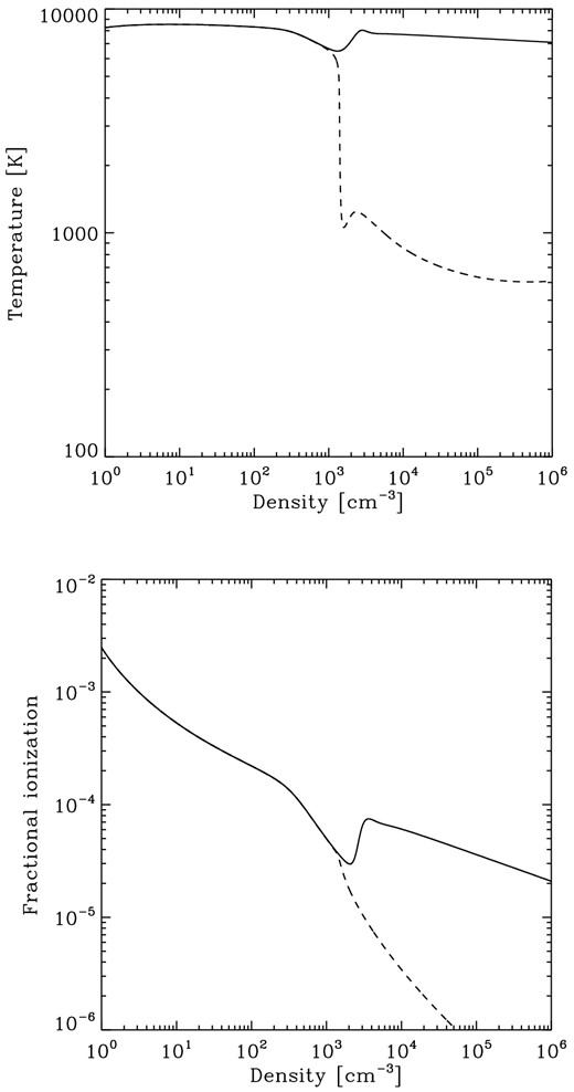
Top panel: evolution of the gas temperature as a function of the hydrogen nuclei number density in runs with the same setup as in run 6 (a T5 spectrum, fully ionized initial conditions). Results are shown for J21 = 1630 (solid line) and J21 = 1635 (dashed line). Bottom panel: evolution of the fractional ionization as a function of density in the same runs.
The value of Jcrit is therefore determined in this case by the chemical state of the gas at n ∼ 103 cm−3 and T ∼ 7500 K. The H2 fraction in the gas in these conditions depends on the fractional ionization. Fig. 1 shows that even though the gas is initially fully ionized, by the time we reach n ∼ 103 cm−3, the fractional ionization has lost its memory of this initial state and has decreased to x ∼ 4 × 10⁻⁵. This value is set by the balance between the collisional ionization of hydrogen by collisions with electrons, H atoms and He atoms (i.e. reactions 12, 10, and 14, respectively) and the radiative recombination of H+. If we compare the rates of reactions 10, 12 and 14 in these conditions, we find that R10 ≃ 4 × 10⁻¹⁶ cm−3 s−1, R12 ≃ 2 × 10⁻¹⁶ cm−3 s−1 and R14 ≃ 10−16 cm−3 s−1. In other words, because of the very low fractional ionization of the gas, reactions 10 and 14 between them provide around 70 per cent of the total collisional ionization rate, with the main contribution coming from reaction 10. Omitting these reactions therefore leads to a factor of ∼3 error in the total ionization rate, and hence a factor of ∼2 error in the fractional ionization. This reduces the H2 formation rate by a similar amount and hence also reduces our estimate of Jcrit.
Another interesting thing that Table 3 shows us is that once we start to look at reactions with lower weights, which are less important overall for our determination of Jcrit, we see substantially more variation from run to run. Only for runs 4 and 5 does our reaction weighting algorithm provide us with exactly the same set of reactions with maximum weights greater than ϵ; for the other runs, we see minor differences, generally involving a small number of processes with weights close to our cut-off. In order to have a reaction network that is robust to changes in the initial conditions and details of the background radiation field, we therefore recommend that one uses all of the 26 reactions listed in Table 3.
3.3 Effect of varying ϵ
In order to establish that our choice of a value of ϵ = 10−4 for the reaction weight cut-off in our selection algorithm does indeed allow us to select all of the reactions important for determining Jcrit, we re-ran our models using a reduced chemical network consisting only of the 26 reactions listed in Table 3 and recalculated Jcrit for each model using the same approach as before. The resulting values are shown in Table 2. We see that there are minor differences in the predicted values of Jcrit in a couple of the runs, but that they are at the level of less than 1 per cent. This is much smaller than the scatter in Jcrit from halo to halo caused by differences in the dynamical evolution of the gas (Latif et al. 2014). This demonstrates that our 26 reaction reduced network is indeed accurate enough for our purposes.
The question then naturally arises as to whether we can simplify our reduced network even more. If we increase the value of ϵ, and hence select even fewer reactions to join the set of ‘important’ reactions, then how badly does this compromise our ability to determine Jcrit accurately? To explore this, we constructed several additional reduced networks, in which we retained only those reactions with maximum weights greater than ϵ = 10−3, 0.01 or 0.1 in at least one run, and then used these even more highly simplified networks to determine Jcrit. When performing this analysis for the ϵ = 0.01 case, we found that in order to produce meaningful results, it was necessary to include one reaction – the destruction of HeH+ by collisions with H, reaction 17 in the table – that formally has a weight that is less than 0.01. The reason for this is that otherwise our ϵ = 0.01 model would contain a reaction that forms HeH+ (reaction 13 in the table), but no reaction that destroys it, meaning that the abundance of HeH+ would increase indefinitely.
The results that we obtained when varying ϵ are shown in columns 4–6 of Table 2. We see that the results we obtain for ϵ = 10−3 or 0.01 are very similar to those we obtain in the ϵ = 10−4 case, with the derived values of Jcrit differing by no more than around 1 per cent. However, in the ϵ = 0.1 case, we see a clear change in behaviour: the error in the value of Jcrit we obtain for the T5 spectrum has increased from ∼1 per cent to a factor of a few. This suggests that if we want to simplify the chemistry as much as possible while still being able to determine Jcrit accurately, then the best choice is a minimal reduced network consisting of reactions 1–15, 17, 22, and 23. On the other hand, if we want to be a little more conservative, in view of the fact that the physical conditions encountered in more realistic simulations are not perfectly reproduced by our one-zone model, then we should retain all 26 of the reactions listed in Table 3.
3.4 Sensitivity to the treatment of H|$_{2}^{+}$| excitation
As we discuss in more detail in the appendix, the rate at which H|$_{2}^{+}$| is destroyed by processes such as dissociative recombination or photodissociation is highly sensitive to the vibrational state of the molecular ions: it is far easier to destroy H|$_{2}^{+}$| ions in states with v ≫ 0 than ones that are in the v = 0 vibrational ground state. Therefore, any model of the chemistry of H|$_{2}^{+}$| in primordial gas should also account, at least approximately, for the degree of excitation of the ions. In the chemical model presented in this paper, this is done in a simple but approximate fashion, for reasons of computational convenience. However, in principle one can construct far more complex and accurate models (see e.g. Coppola et al. 2011). An obvious question is therefore whether this complexity is necessary if one wants to accurately determine Jcrit, or whether the simple treatment used in this paper suffices.
To answer this question, we performed two additional sets of runs. In the first set, we artificially set the H|$_{2}^{+}$| critical density to a very large number, so that all of the chemical rates used for the ion were the ones for H|$_{2}^{+}$| in its ground state. In the second set of runs, we instead set the H|$_{2}^{+}$| critical density to zero, so that the local thermodynamic equilibrium (LTE) rates were used for all of the reactions involving H|$_{2}^{+}$| as a reactant. These two limiting cases should bracket the real behaviour of the H|$_{2}^{+}$| ions in the gas, and so by comparing the results of these two sets of runs, we can establish how sensitive Jcrit is to the details of the excitation of the H|$_{2}^{+}$| ions.
We show the results from these two sets of runs in Table 4, along with the results from our fiducial model for comparison. We see that there is only a small difference between the values of Jcrit that we obtain using our fiducial model and those from the v = 0 model. This is not surprising, since the question of whether or not enough H2 forms to cool the gas is largely determined by the chemistry occurring at densities n < ncrit, where the v = 0 rates are a good approximation. If we instead adopt LTE rates throughout, we find a larger difference between the models, approximately 20 per cent in the runs with the T4 spectrum and ∼5 per cent in the runs with the T5 spectrum. As this represents a worst case, the real error introduced is almost certainly smaller than this. Our simplified treatment of H|$_{2}^{+}$| excitation therefore does not represent a major source of error in our determination of Jcrit.
Dependence of Jcrit on our treatment of H|$_{2}^{+}$| excitation.
| Jcrit | |||
|---|---|---|---|
| Run | Fiducial | v = 0 | LTE |
| 1 | 17.0 | 17.6 | 14.2 |
| 2 | 18.0 | 18.6 | 14.5 |
| 3 | 18.0 | 18.6 | 14.5 |
| 4 | 1640 | 1650 | 1560 |
| 5 | 1630 | 1640 | 1560 |
| 6 | 1630 | 1640 | 1560 |
| Jcrit | |||
|---|---|---|---|
| Run | Fiducial | v = 0 | LTE |
| 1 | 17.0 | 17.6 | 14.2 |
| 2 | 18.0 | 18.6 | 14.5 |
| 3 | 18.0 | 18.6 | 14.5 |
| 4 | 1640 | 1650 | 1560 |
| 5 | 1630 | 1640 | 1560 |
| 6 | 1630 | 1640 | 1560 |
3.5 Importance of dissociative tunnelling
Our analysis in Section 3.2 showed that the collisional dissociation of H2 has one of the largest weights in our reduced chemical network, and therefore it is very important to treat this process accurately. As discussed at some length in e.g. Martin, Schwarz & Mandy (1996), there are two distinct processes that contribute to the total collisional dissociation rate. The first is direct collisional dissociation, where the H2 molecule undergoes a transition from a bound state directly into the continuum of classically unbound states. The second is dissociative tunnelling, where the H2 molecule is excited into a quasi-bound state – a state that has an internal energy larger than is required for dissociation, but which is separated from the continuum by a barrier in the effective potential. Quantum tunnelling through this barrier then leads to spontaneous dissociation. In low-density gas this process of dissociative tunnelling can make a major contribution to the total collisional dissociation rate.
Some studies of the direct collapse model for the formation of massive black holes include only the effects of direct collisional dissociation, and not those of dissociative tunnelling (e.g. Shang et al. 2010), but as Latif et al. (2014) point out, this potentially introduces significant uncertainty into the resulting values derived for Jcrit. In an effort to quantify this uncertainty, we re-ran our set of six simulations using our reduced chemical model, but with the effects of dissociative tunnelling disabled. We found that in this case, Jcrit = 33.1 in runs 1–3 and Jcrit = 2780 in runs 4–6. In other words, the failure to account for this process when modelling H2 dissociation in this scenario can introduce an error of almost a factor of 2 into Jcrit.
3.6 Comparison with other chemical models
It is interesting to investigate whether there are any significant differences between the reduced chemical network constructed in this paper and the other chemical networks in common usage in studies of the direct collapse model for the formation of massive black holes. The majority of existing studies use one of three treatments: the krome astrochemistry package (Grassi et al. 2014), which provides a range of different networks for modelling primordial chemistry; the primordial chemistry network implemented in the enzo adaptive mesh refinement code, described in Bryan et al. (2014), which is a modified and extended version of the network outlined in Abel et al. (1997); or the network introduced in Omukai (2001). We compare our reduced network to each of these treatments below.
3.6.1 The krome package
The krome astrochemistry package is a python-based pre-processing system that converts a simple textual description of an astrochemical network into a set of subroutines for the solution of the chemical rate equations for the species contained in that network. In addition, krome also contains support for a large number of different heating and cooling processes, allowing the thermal energy equation to be solved along with the chemical rate equations. krome is still undergoing active development, but in our discussion here we refer to the state of the code at the time of writing;2 note that this differs in some respects from the previous version of the package described in Grassi et al. (2014).
The krome package provides a number of example networks, including several designed for modelling primordial gas. Unfortunately, these come with very little documentation, and so it is not immediately obvious which network is the best choice for which application, or even which (if any) of these networks has been used in studies such as Latif et al. (2014), Van Borm et al. (2014), or Latif et al. (2015) that have been carried out using krome. However, some investigation allows us to immediately cut down the number of possibilities. We can clearly ignore any of the primordial networks that do not include the photodissociation of H− or H2, since these are crucial processes in the case of the T4 or T5 spectra, respectively. This leaves us with only two networks to consider: the react_primordial_photoH2 network and the react_xrays network.
The react_primordial_photoH2 network consists of reactions 1–8, 11, 12, 15, 22, 23, 25, and 26 from our reduced network, along with several additional reactions, largely involving the ionization and recombination of helium and the chemistry of D, D+, and HD, which our results demonstrate are not important for the determination of Jcrit. The react_xrays network consists of the reactions mentioned above, plus two more from our reduced network, reactions 9 and 18. It also accounts for charge transfer between hydrogen and helium, and includes a more extensive treatment of deuterium chemistry, but once again, our results suggest that these processes are unimportant for determining Jcrit.
We therefore see that compared to our reduced network, the react_xrays network is missing reactions 10, 13–14, 16–17, 19–21, and 24, while the react_primordial_photoH2 network is missing these plus also reactions 9 and 18. To quantify the effect of omitting these reactions on the determination of Jcrit, we have rerun our set of six simulations using only the reactions contained in the react_xrays network, and determined the value of Jcrit in each case. Note that when doing so, we use the rate coefficients for each reaction taken from our chemical model, which are not always the same as those adopted by the krome model. This is because we are interested here only in the effects of omitting some of the reactions that we have determined are important, and not on quantifying the uncertainty introduced into Jcrit by differences in our choice of rate coefficients. We examine the latter issue at some length in a companion paper (Paper II).
The results of our comparison are shown in Table 5. We see that the krome network systematically underestimates Jcrit. The discrepancy is worst in run 1, where the error is almost a factor of 2, but even in the best case, the error is ∼20 per cent. We have also carried out a similar comparison using the set of reactions in the react_primordial_photoH2 network, but find that in this case we recover very similar results. We have investigated the source of this discrepancy and find that almost all of it is accounted for by the omission of reactions 10 and 14 from the krome model. If we add these two reactions to the set included in the react_xrays network, then we can reproduce the values of Jcrit that we obtain with our minimal model to within ∼1 per cent.
Comparison of Jcrit determined using our reduced model with that determined using several other simplified models from the literature.
| Jcrit | ||||
|---|---|---|---|---|
| Run | This work | krome | enzo | Omukai (2001) |
| 1 | 17.1 | 8.9 | 21.5 | 17.1 |
| 2 | 18.0 | 14.7 | 26.7 | 18.3 |
| 3 | 18.1 | 14.9 | 26.8 | 18.3 |
| 4 | 1640 | 1120 | 1930 | 3040 |
| 5 | 1630 | 1160 | 1940 | 3040 |
| 6 | 1630 | 1160 | 1940 | 3040 |
| Jcrit | ||||
|---|---|---|---|---|
| Run | This work | krome | enzo | Omukai (2001) |
| 1 | 17.1 | 8.9 | 21.5 | 17.1 |
| 2 | 18.0 | 14.7 | 26.7 | 18.3 |
| 3 | 18.1 | 14.9 | 26.8 | 18.3 |
| 4 | 1640 | 1120 | 1930 | 3040 |
| 5 | 1630 | 1160 | 1940 | 3040 |
| 6 | 1630 | 1160 | 1940 | 3040 |
3.6.2 The enzo network
The primordial chemistry network implemented in the enzo code consists of the same subset of the reactions from our minimal model as in the kromereact_xrays network, i.e. reactions 1–8, 11, 12, 15, 22, 23, 25, and 26. As in the case of the krome networks, it also includes a number of reactions involving the ionization and recombination of helium and the chemistry of deuterium that play no role in the determination of Jcrit. The only difference between the enzo network and the kromereact_xrays network that is relevant for this study is that the krome network accounts for the collisional dissociation of H2 via dissociative tunnelling as well as direct dissociation into the continuum, whereas the enzo model only includes the latter process.
In Table 5, we compare the values of Jcrit that we obtain using the enzo model with those that we obtain using our reduced model. We find that the enzo model systematically overestimates Jcrit by between 20 and 50 per cent. Interestingly, the mean difference is smaller than with the krome model, despite the fact that the enzo model is less complete than the krome model. The reason for this is that while the neglect of reactions 10 and 14 in the enzo model tends to decrease our estimate of Jcrit, the neglect of dissociative tunnelling has the opposite effect, as we have seen already in Section 3.5. Therefore, the two effects cancel to some extent, and so the overall difference with the results of our reduced model is less than we would initially expect.
3.6.3 The Omukai (2001) network
The chemical network adopted by Omukai (2001) in his pioneering study of the effects of a strong extragalactic radiation field on the gravitational collapse of primordial gas includes reactions 1–10, 12, 15, 18, 22, and 26 from our reduced network. It also includes a number of additional reactions such as the three-body recombination of H+, or the collisional ionization of electronically excited hydrogen that are unimportant at the densities at which the value of Jcrit is set, but which play important roles in regulating the ionization state and thermal evolution of the gas at much higher densities. The Omukai (2001) network, which for the sake of brevity we refer to hereafter as the O01 network, or an updated version of it, has subsequently been used in a number of different studies of aspects of the direct collapse model for black hole formation (e.g. Omukai et al. 2008; Inayoshi & Omukai 2011, 2012; Inyoshi, Omukai & Tasker 2014; Sugimura, Omukai & Inoue 2014).
In Table 5, we compare the results we obtain for Jcrit when we use the set of reactions contained in the O01 network with the values obtained using our reduced network. In performing this comparison, we have assumed that the O01 network accounts for both the direct collisional dissociation of H2 and its destruction by dissociative tunnelling. This was not the case in the original version of the network, which used a highly outdated treatment of H2 collisional dissociation taken from Lepp & Shull (1983). More recent studies use an updated treatment based on Martin et al. (1996), but do not clarify whether they include only the direct collisional dissociation or also the dissociative tunnelling term.
We see from Table 5 that there is very good agreement between the results of our reduced network and those obtained using the O01 network in the case of the simulations performed using the T4 spectrum. In these runs, the maximum difference between the two models is around 2 per cent. The main reason that the O01 model performs much better than the krome or enzo models in this case is that it includes the effects of reaction 10, which, as we have already seen, significantly contributes to the ionization state of the gas at the densities where the value of Jcrit is set.
4 SUMMARY
In this paper, we have attempted to identify the set of chemical reactions that it is essential to include in any chemical network used to determine Jcrit, the critical UV flux required to suppress H2 cooling in atomic cooling haloes with Tvir > 104 K. To do this, we have made use of the reaction-based reduction algorithm developed by Wiebe et al. (2003). This has previously been applied to the study of the chemistry of the local interstellar medium, but to the best of our knowledge, this paper marks its first use in the study of the chemistry of primordial gas.
Using this reduction technique with a conservative choice of ϵ = 10−4 for the reaction weight below which we do not retain reactions in our reduced network, we find that we can reduce our initial 30 species, ∼400 reaction network to a reduced network containing only eight chemical species linked by 26 reactions. We have verified that simulations carried out using this reduced network predict essentially identical values of Jcrit to those carried out using our full network. We have also explored the effect of varying ϵ, and find that we continue to be able to predict Jcrit accurately as long as ϵ ≤ 10−2. Setting ϵ = 10−2 allows us to produce an even smaller ‘minimal’ reduced network, containing the same set of eight chemical species, but now linked by only 18 reactions.
To put this number into context, we note that in the regime relevant for the direct collapse model, the probability of an atomic cooling halo being exposed to a local radiation field with a strength J21 > Jcrit is a strongly decreasing function of Jcrit (Dijkstra et al. 2014). For example, Inayoshi & Tanaka (2014) show that for 103 < Jcrit < 104, this probability scales approximately as |$P \propto J_{\rm crit}^{-5}$|. A factor of 3 uncertainty in Jcrit can therefore potentially correspond to a factor of ∼200 uncertainty in the cosmological number density of massive black holes formed by direct collapse.
Finally, we stress that this uncertainty can be eliminated from future studies of the direct collapse model simply by ensuring that the chemical network adopted includes the full set of chemical reactions that are important for determining Jcrit. We therefore recommend that in future work, researchers take care to include, at the very least, all of the reactions making up the minimal reduced model described in Section 3.3.
The author would like to thank T. Hartwig, S. Khochfar, R. Klessen, and M. Volonteri for useful conversations regarding the physics of black hole formation in the high-redshift Universe. Additional thanks also go to T. Hartwig for his comments on an earlier draft of this paper. Special thanks go to B. Agarwal and B. Smith for several discussions regarding the possible impact of chemical uncertainties on Jcrit that inspired the author to carry out the work described here. Financial support for this work was provided by the Deutsche Forschungsgemeinschaft via SFB 881, ‘The Milky Way System’ (subprojects B1, B2, and B8) and SPP 1573, ‘Physics of the Interstellar Medium’ (grant number GL 668/2-1), and by the European Research Council under the European Community's Seventh Framework Programme (FP7/2007-2013) via the ERC Advanced Grant STARLIGHT (project number 339177).
Specifically, on 2015 January 03, at which time the most recent commit was 53a32c2ab5d53994fe4893676dbfbcf08125c23d.
REFERENCES
APPENDIX A: REVISIONS TO THE THERMAL MODEL
We have improved on the thermal model introduced in Glover & Abel (2008) and Glover & Savin (2009) by updating the rates of two of the cooling processes in an effort to use the most up-to-date data available. Details of our changes are given below.
A1 Updated cooling rates
A1.1 Collisional excitation of H2 by electrons
A1.2 Collisional excitation of H2 by protons
APPENDIX B: REVISIONS TO THE CHEMICAL MODEL
We have improved on the chemical model introduced in Glover & Savin (2009) by including three new reactions and updating the reaction rates used for a further eight reactions. Details of our changes are given below.
B1 New reactions
B1.1 Collisional ionization of atomic hydrogen
In practice, trapping of Lyman α photons in the collapsing gas owing to the high optical depth in the Lyman α line leads to the existence of a non-zero population of hydrogen atoms in excited electronic states (see e.g. Omukai 2001; Schleicher et al. 2010). However, at the densities of interest in this study, only a very small fraction (of order 10−10 or less) of the total number of hydrogen atoms are found in these states (Schleicher et al. 2010), and so there is no need to account in the chemical model for the effects of collisional ionization out of these states.
B1.2 Collisional dissociation of H|$_{2}^{+}$| by atomic hydrogen
Although this is a somewhat crude approximation, it is sufficient for our purposes, since Jcrit is not very sensitive to the treatment adopted for H|$_{2}^{+}$| excitation (see Section 3.4).
B2 Updated reaction rates
Since the publication of Glover & Savin (2009), new experimental and/or theoretical data has become available for a number of different reactions. We have therefore updated the rates adopted for several of the included reactions, as detailed below.
B2.1 Associative detachment of H− with H
B2.2 Mutual neutralization of H− with H+
B2.3 Dissociative recombination of H|$_{2}^{+}$|
B2.4 Collisional dissociation of H2 by H
B2.5 Charge transfer from H+ to H2
B2.6 Three-body formation of H2
B2.7 Photodissociation of H|$_{2}^{+}$|
B2.8 Formation of H|$_{2}^{+}$| by radiative association
The fit gives values for the rate coefficients that agree with those tabulated by Ramaker & Peek (1976) to within around 5–6 per cent. Moreover, at the temperatures most relevant in this study, T ∼ 4000–8000 K, the agreement is even better, with the fit differing from the tabulated values by no more than 1–2 per cent.
