


Abstract
Computations of chromospheric models and the resulting spectral line emission fluxes are presented for late-type stars exhibiting very low level of chromospheric activity, referred to as a basal flux stars or low activity stars. The computations are self-consistent, and consider the entire acoustic wave energy spectra generated in the stellar convection zones. We consider multilevel atomic models, take into account departures from local thermodynamic equilibrium and also consider the time-dependent ionization processes of hydrogen. We employ the new finding of the mixing-length parameter α = 1.8. The Ca ii H+K and Mg ii h+k line fluxes are computed assuming pseudo-partial redistribution. The results show the importance of time-dependent ionization in modelling the middle and high chromospheres. Models without considering time-dependent ionization overestimate the emitted Ca ii fluxes by factors between 1.1 and 5.6 for F8V and M0V stars, respectively, while factors between 1.8 for G0V and 17.4 for M0V stars have been obtained for the Mg ii fluxes. The theoretically computed basal fluxes in Ca ii and Mg ii, respectively, follow simple linear formulae depending on the effective temperature log Teff. The obtained results for Ca ii fluxes show reasonable agreement with observations.
1 INTRODUCTION
Solar and stellar chromospheric activities can be studied through the emissions in the Ca ii H+K and Mg ii h+k spectral lines with their temperature sensitive emission peaks being directly correlated with the magnetic activities. A linkage between solar Ca ii H+K emission and activity was first suggested by Eberhard & Schwarzschild (1913), Howard (1959) and Leighton (1959) found a correlation between Ca ii H+K emission and magnetic flux density on the solar surface, concluding that the radiative losses from the outer layers of the Sun depend on the magnetic flux density of the underlying photosphere. The Sun provides us with detailed observations because of the high spatial resolution, while observing stars give us a wide range of basic parameters (i.e. mass, age, rotation rate, and composition) which are important for studying the parameters affecting the stellar activities. Schrijver, Dobson & Radick (1989) classified the Mount Wilson Ca ii H+K fluxes of cool dwarf stars into two main components: (1) a basal component which is independent of stellar magnetic fields or rotation, and thought to be of nonmagnetic origin, (2) a component which is related to the magnetic activity and rotation. Inactive and slowly rotating stars have basal chromospheres, while active stars have both components.
Now, it is widely accepted that the dissipations of different wave modes (e.g. acoustic, longitudinal magnetic flux tube, transverse, and Alfvèn waves) are partially responsible for the observed outward temperature rise in stellar atmospheres. Recent analysis of measurements obtained by the Swedish 1 m Solar Telescope (Freij et al. 2014) show signature of ‘upwardly propagating field-aligned waves’. Stangalini et al. (2011) have shown that acoustic waves can be converted to magnetoacoustic waves in the photosphere and propagate upwardly into the chromosphere. The detections of magnetic fields for giant and supergiant stars support the correlation between the magnetic field and the heating of stellar outer layers (Konstantinova-Antova et al. 2010, 2012).
In 2009, the Sun reached its extreme minimum activity with S-index (Mount Wilson S-index to measure the activity level) coincided with the S-indices of flat activity stars (possibly identical to Maunder Minimum stars). This comparison suggested a universal heating mechanism for the chromospheres of inactive stars (see e.g. Pérez Martinez, Schröder & Cuntz 2011; Pérez Martinez et al. 2014; Schröder et al. 2012). In a study by Sobotka et al. (2014), acoustic waves have been found to contribute to 25–50 per cent of the energy radiated by the quiet chromosphere and plage regions, respectively, see also studies by Ulmschneider (1991), Cuntz, Rammacher & Ulmschneider (1994), Buchholz, Ulmschneider & Cuntz (1998), and Pérez Martinez et al. (2011).
Now, the important questions are what energy sources exist and how to correlate the different sources with the heating of the atmospheric layers of different activities? Simple answers to these questions require knowledge of the waves with different modes and their dependence on the degree of magnetic activity, where the type of interaction between the magnetic field lines and the plasma generates different wave modes.
We can thus propose that non-magnetic regions or magnetic-inactive stars showing basal chromospheres are heated by the dissipation of acoustic waves independent on rotation, and can be best modelled only by the effective temperature, gravity, and metallicity.
The importance of the magnetic and acoustic heating vary from star to star and from one position to another on the stellar surface. Some areas on stellar surfaces are dominated by strong fields while others are either field-free or contain weak fields. Because of the lack of spatial resolution, observations do not show these regions separately, so it is not easy to distinguish between the different mechanisms. The observed flux–colour diagrams of the chromospheric Mg ii h+k and Ca ii H+K surface flux densities (e.g. Rutten et al. 1991; Vilhu 1987) show clear lower limits in |$F_{\rm Mg\,\small {II}}$| and |$F_{\rm Ca\,\small {II}}$|, and scatter of data with more emission above this boundary. The lower limit is determined by the least active stars. Magnetic braking through the magnetized stellar wind decelerates the stellar rotation, which results in a steady loss of the angular momentum throughout the stellar age. Old stars are slow rotators while young stars are rapid rotators. As the efficiency of the generation of magnetic field increases with stellar rotation rate and the depth of the convection zone (dynamo mechanism), we expect that the lower limits of Mg ii and Ca ii emission fluxes are determined by old, slowly rotating stars. In our models, the basal chromospheres (the voids between flux tubes) are heated by the dissipation of acoustic waves, and magnetic regions are heated by the dissipation of longitudinal and other tube waves. The two atmospheres are combined together in one model to compute the emitted Mg ii and Ca ii fluxes.
The reason to revisit this problem is fourfold, the use of wider and more realistic wave energy spectra, the consideration of the time-dependent ionization of hydrogen, the multilevel radiation treatment of Mg ii and Ca ii spectral lines, and the recent value of the mixing-length parameter α = 1.8 for modelling the convection zone, obtained from calibrations of the classical mixing-length and realistic 3D hydrodynamic simulations (Trampedach et al. 2014). The importance of time-dependent ionization in modelling the solar chromosphere and its effect on the emitted Mg ii and Ca ii has been extensively studied (e.g. Carlsson & Stein 1992, 1995).
Our paper is organized as follows: the problem is formulated in Section 2 and the method used to solve the problem is also described there; in Section 3, we present the obtained results and discuss them; our conclusions are given in Section 4.
2 METHOD OF COMPUTATION
In the current approach the vertical structure of stellar atmospheres is modelled. The problem is divided into two coupled modules: the first deals with the wave generation, the second one handles the wave propagation and dissipation. Detailed information on the algorithms used in the current computations is given in Appendix A. The following subsections briefly summarize the numerical approach.
2.1 Stellar parameters and the initial atmospheres
Updated stellar parameters for theoretical late-type stars have been deduced by Gray (2005). These values, notably Teff and log g (see Table 1), serve as the basis for the present study. The current models are computed using the solar chemical abundances, i.e. abundance by mass of hydrogen Xm = 0.70, helium Ym = 0.28, and of metals Zm = 2x10− 2. The computations start by constructing a grey radiative equilibrium plane parallel atmosphere for a given effective temperature Teff and gravity g, using a temperature correction method by Cuntz et al. (1994). A non-grey radiative equilibrium model atmosphere, which includes NLTE and the Mg ii k line, has been constructed and the resulting atmosphere has a temperature gradient that decreases outwards. The bottom of the model is taken at height z = 0 km, where the external optical depth is τ5000 = 1.
2.2 Wave energy fluxes and spectra
The input acoustic wave energy fluxes and spectra generated at the top level of the convection zones were computed following the procedure described by Ulmschneider, Theurer & Musielak (1996). Table 1 lists the input parameters used for constructing the model chromospheres of late-type stars. The procedure is based on the classical mixing-length theory and allows computing the acoustic wave energy fluxes for a broad range of stars with different effective temperatures, surface gravities, and metal abundances.
The parameters used in the current study for the late-type stars with different effective temperatures Teff, gravity log g, and the acoustic wave energy flux Fac computed for each star.
| Star | B − V | Teff | log g | Fac |
|---|---|---|---|---|
| – | (mag) | (K) | – | (erg cm−2 s−1) |
| F8V | 0.46 | 6160 | 4.355 | 2.5E8 |
| G0V | 0.58 | 5943 | 4.360 | 1.6E8 |
| G2V | 0.65 | 5811 | 4.368 | 1.3E8 |
| G5V | 0.68 | 5657 | 4.443 | 8.5E7 |
| K2V | 0.89 | 5055 | 4.558 | 1.8E7 |
| M0V | 1.40 | 3850 | 4.783 | 3.4E5 |
The acoustic waves are generated by turbulent convection, and turbulence is modelled by an extended form of Kolmogorov spectrum with a modified Gaussian frequency factor (Musielak et al. 1994). The calculations performed by these authors showed that a choice of the mixing-length parameter α strongly affects the values of the acoustic fluxes. In the solar application, it is possible to select many model parameters and characteristic values directly from observations. However, for stars other than the Sun such data are mostly unavailable.
The 2D or 3D radiation hydrodynamic simulations of stellar convection and mixing-length models show that the maximum convective velocities occur at optical depths of τ5000 = 10–100. For example, Steffen (1993) found in his time-dependent solar numerical convection calculations that maximum convective velocities vCMax ≈ 2.8 km s−1 are reached at τ5000 ≈ 50 and that these values can be reproduced by the mixing-length theory with a mixing-length parameter of α ≈ 2. Additionally, state-of-the-art solar convection zone simulations by Stein et al. (2009a,b) encompassing the scale of super granules concluded that the behaviour of solar convection is consistent with the mixing-length parameter of about α = 1.8. Recent calibrations of the classical mixing length by Trampedach et al. (2014) against 3D radiation hydrodynamic simulations show a clear plateau of α ≈ 1.76.
From the above, one can conclude that recent simulations are in principle consistent with the mixing-length concept (in the case of selected features of convection) and that the wave energy flux is well defined for a given star if the mixing-length parameter α can be specified. For these reasons, in our study we consider the value of α = 1.8 for the mixing-length parameter.
A comparison of the resulting wave energy flux spectra is shown in Fig. 1.
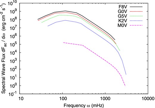
The generated acoustic wave energy spectra dFac/dω for F8V, G0V, G5V, K2V, and M0V type stars.
2.3 Hydrodynamic equations
The system of equations is solved using the method of characteristics as explained in detail by Rammacher & Ulmschneider (2003). This code allows computing one-dimensional time-dependent wave propagation in stellar atmospheres while incorporating the treatment of hydrogen ionization by solving the time-dependent statistical rate equations. The time-dependent hydrodynamic equations are solved for an atmospheric slab by using the method of characteristics; furthermore, the thermodynamical relationships as well as the Rankine–Hugoniot relations across the shocks are also solved in a self-consistent time-dependent manner. The solutions are obtained together with an evaluation of the radiation losses under departures from local thermodynamic equilibrium (NLTE).
Fig. 2 shows an example of the velocity fluctuations u(z = 0, t) at stellar surface of a G0V star.
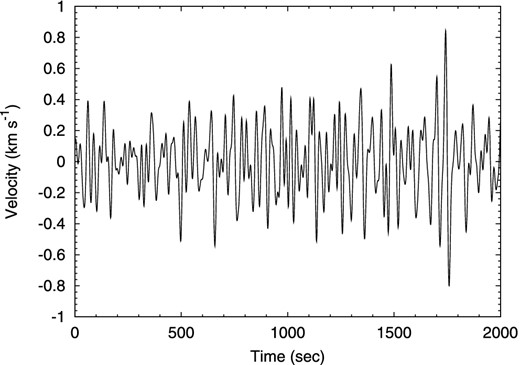
The gas velocity fluctuations, computed from equation (4), at the stellar surface of a G0V type star.
The top boundary condition is a transmitting boundary. Upon the propagation of the waves in an outer atmosphere with a decreasing density, shocks can form with different strengths which depend on the input mechanical wave energy and wave period. Shocks are treated as discontinuities. The input mechanical energy flux also affects the shock formation heights, it has been found that when increasing the input mechanical energy flux one has stronger shocks which form at lower heights of the atmospheres (see Fawzy, Ulmschneider & Cuntz 1998; Fawzy & Cuntz 2011).
In the framework of our models, we consider time-dependent ionization with respect to hydrogen. It is our aim to represent the total chromospheric emission losses, the Ca ii K and Mg ii k lines are scaled accordingly to represent the total chromospheric emission function using the multilevel atomic models as will be explained later.
2.4 Time-dependent ionization
The hydrogen ionization greatly affect the electron densities in the chromosphere and are directly used for the computations of the collisional rate transitions.
2.5 The multilevel atomic models
Accurate representation of the time-dependent energy balance in chromospheric wave calculations require computation of the emitted radiative losses of the major sources of the main chromospheric lines hydrogen, Ca ii, Mg ii, and Fe ii (Vernazza, Avrett & Loeser 1981; Anderson & Athay 1989). The current computations are based on the methods developed by Rammacher et al. (2005) and recent results by Fawzy (2015). The method is based on multiplying single Ca ii K and Mg ii k line emission fluxes with radiation correction factors obtained by comparing the two-level atomic model with that of a multilevel model. The line profiles are calculated assuming complete redistribution (CRD) and using a reduced damping parameter to simulate the effects of PRD (pseudo-PRD, see Fig. 3). A five-level atomic model for Ca ii (K, H, IRT lines) plus continuum is used, the Mg ii h+k lines and continuum are represented by a three-level model.

The computations start by solving the hydrodynamic equations simultaneously with the radiative transfer equations using the two-level atom approach (rad2l). With the specification of initial values for the correction factors, the rad2l code is allowed to run for enough time until the atmosphere reaches hydrostatic equilibrium. Different phases of the heated atmosphere with the inserted shocks together with the two-level based radiative losses are then exported and used as input for the multilevel computations (multi-code). The multi-code recomputes the multilevel damping functions (K, H, and IRT lines for Ca ii plus continuum and the k, h, plus continuum for Mg ii) and compares the results with those obtained by the rad2l code. The process is iteratively repeated until the difference between two successive iterations is very small. The values are usually converge after two to three iterations. The obtained factors are shown in Table 2 .
The radiation correction factors for Ca ii and Mg ii ions.
| Star | |$R_{\rm Ca\,\small {II}}$| | |$R_{\rm Mg\,\small {II}}$| |
|---|---|---|
| F8V | 4.88 | 1.50 |
| G0V | 5.92 | 1.48 |
| G2V | 5.02 | 1.52 |
| G5V | 5.33 | 1.50 |
| K2V | 5.23 | 1.51 |
| M0V | 6.07 | 1.51 |
| Star | |$R_{\rm Ca\,\small {II}}$| | |$R_{\rm Mg\,\small {II}}$| |
|---|---|---|
| F8V | 4.88 | 1.50 |
| G0V | 5.92 | 1.48 |
| G2V | 5.02 | 1.52 |
| G5V | 5.33 | 1.50 |
| K2V | 5.23 | 1.51 |
| M0V | 6.07 | 1.51 |
The basal Mg ii and Ca ii fluxes for late-type stars.
| Star | Fac | |$F_{\rm Mg\,\small {II}}$| | |$F_{\rm Ca\,\small {II}}$| |
|---|---|---|---|
| – | (erg cm−2 s−1) | (erg cm−2 s−1) | (erg cm−2 s−1) |
| F8V | 2.5E8 | 6.0E5 | 6.4E5 |
| G0V | 1.6E8 | 2.8E5 | 5.0E5 |
| G2V | 1.3E8 | 4.2E5 | 5.5E5 |
| G5V | 8.5E7 | 2.9E5 | 5.1E5 |
| K2V | 1.8E7 | 2.4E5 | 3.3E5 |
| M0V | 3.4E5 | 2.8E4 | 2.0E4 |
2.6 PRD treatment
Strong lines formed in non-LTE where the collision rates very low because of the very low gas density (the radiative transitions are more dominant over the collisional rates). This requires considering partial redistribution by photons (PRD). At the formation heights of the Mg ii and Ca ii lines, the assumption of CRD overestimates the radiative loss rates of spectral lines by more than an order of magnitude (see Hünerth & Ulmschneider 1995). The assumption of PRD should be combined with multilevel atomic model in the time-dependent computations. A fast and reasonably accurate CRD-based method called pseudo-PRD has been suggested by decreasing the damping factor a in the Voigt function by factors 100 and 1000 (see e.g. Uitenbroek 2001, 2002). Fig. 3 shows a comparison for Mg ii k line from our two-level computations by decreasing the damping parameter by factors of 100 and 1000 with the model C of Vernazza et al. (1981) and with real PRD computations. Good agreement is obtained for the case which has a reduced damping parameter by factor of 100. This method is very reasonable and fast enough to be implemented in the current time-dependent computations.
3 RESULTS AND DISCUSSION
3.1 Time-dependent model simulations
The acoustic computations start from undisturbed models with outward decreasing temperatures. These initial atmospheres extend up to 3300 and 900 km for F8V- and M0V-type stars, respectively. The wave energy fluxes and spectra are introduced at a height z = 0 km by means of a piston. The wave propagations are followed and the balance between the energy dissipation by shocks and radiative losses by chromospheric emitters are computed self-consistently. The computations are carried out until about 40–50 shocks are transmitted through the top boundary of the atmosphere. These numbers have been found to be enough for the atmosphere to reach a dynamical equilibrium between heating by shocks and the radiative cooling. Also by this time the switch-on effects caused by start of the waves has disappeared. At this point, the time-averaged quantities do not change with time, and different wave phases are used for the computation of accurate radiation fluxes using multilevel atomic models and applying the PRD treatment.
Fig. 4 shows a snapshot of an acoustic model for a G0V star at elapsed time t = 2487 s. Shocks start forming at height near z = 700 km, above this height, the shock amplitudes show significant increase, and thus noticeable jumps in temperature. The obtained post-shock temperature is about 12 500 K at height z = 2500 km with a shock strength of Ms = 2.54.
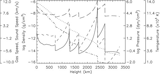
A snapshot of acoustic wave computations for a G0V star taken at time t = 2487 s. The temperature (solid line), the velocity (dashed lines), the density (short dashed lines), the sound speed (long dashed lines), and the pressure (dash–dotted lines) are shown.

3.2 Basal Ca ii and Mg ii fluxes
In a two-component chromosphere (magnetic and nonmagnetic), one heating mechanism may be more dominant than the other, but both mechanisms work together even for the least active stars which might still have a remaining magnetic activity from a residual dynamo effect or from a background, non-variable turbulent dynamo (e.g. Saar 1998; Schrijver et al. 1998; Bercik et al. 2005). If we assume that the magnetic heating mechanism does not contribute to the heating of the outer layers of low activity slowly rotating stars or stars at the minimum activity cycle, one can construct chromospheric models based on a purely acoustic heating mechanism.
Theoretical chromospheric models based only on acoustic heating, have been constructed by Buchholz et al. (1998) for main-sequence stars between spectral types F0V and M0V and two giants of spectral types K0III and K5III. These computations were based on monochromatic acoustic waves. A comparison of the computed Mg ii h+k and Ca ii H+K fluxes with the lower limit of the flux–colour diagram presented by Rutten et al. (1991) (see Figs 5 and 6) showed good agreement over nearly two orders of magnitude. Theurer (1998) used acoustic wave spectra instead of monochromatic waves and found that heating the outer layers of late-type stars with wave spectra results in a small number of shocks with very large strengths and therefore larger emission fluxes relative to the monochromatic waves. The computed time-averaged fluxes of Mg ii and Ca ii lines by Theurer (1998) are larger than the observed basal flux line of Rutten et al. (1991); this is explained by the higher jumps of a shock with the higher post shock temperatures and the lack of treating the non-instantaneous ionization. On the other hand, Theurer (1998) has neglected the inclusion of time-dependent ionization which has been found to be important with the use of wave spectra.
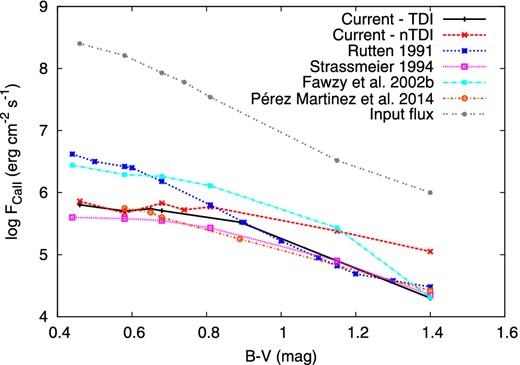
Our computed Mg ii h+k and Ca ii H+K flux losses from one-component acoustically heated chromospheres with the consideration of time-dependent ionization show better matching with observations. The computed PRD emission fluxes of the Ca ii H+K and Mg ii h+k lines are compared with the lower limit of the flux–colour diagram of Rutten et al. (1991) and with an average observed minimum fluxes of Strassmeier et al. (1994) (only for Ca ii H+K fluxes).
Figs 5 and 6 show how the computed total emission flux relates to the acoustic input fluxes in comparison with observations. Table 3 summarizes the obtained results. The computed total emission flux (Ca ii + Mg ii) depends on B − V (B − V = 15.7 − 4logTeff; Böhm-Vitense 1981). The obtained fluxes show a monotonic decrease as a function of B − V. Hot stars (small B − V) show more emission than cool stars (large B − V).
An explanation for the difference between the mechanical input energy and the total Mg ii + Ca ii line fluxes is that in the computation of the energy balance between shock heating and the chromospheric radiation losses also other cooling mechanisms such as e.g. H− were taken into account in the wave code.
3.3 Effect of time-dependent ionization
The statistical equilibrium equations appear not to be valid under the very dynamic conditions of the solar and stellar chromospheres. The processes that are responsible for the ionization and recombination rates change as a function of height through the chromosphere as a result of the interplay between shock strengths and the local properties of the medium (for more details, see e.g. Carlsson & Stein 2002).
With the consideration of time-dependent ionization for hydrogen, we constructed theoretical models based on realistic acoustic wave energy fluxes and spectra. The use of wave spectra lead to formation of a small number of shocks compared to the monochromatic waves, but with higher strengths. The treatment of these shocks requires the consideration of time-dependent ionization (see e.g. Rammacher & Ulmschneider 2003; Fawzy & Cuntz 2012).
The results shown in Figs 5 and 6 shed the light on the importance of the time-dependent ionization for constructing stellar chromosphere models. If the time-dependent is assumed, the obtained fluxes match better with the observations.
If we neglect time-dependent ionization, the strength of the strong shocks is overestimated because of which the simulated Ca ii and Mg ii emission lines and the basal flux line is too high (Ulmschneider et al. 2005). The results of the models without time-dependent ionization show increase in Ca ii fluxes by factors between 1.1 and 5.6 for F8V and M0V stars, respectively. The effect is more pronounced for Mg ii, where the fluxes increase by factors between 1.8 for G0V and 17.4 for M0V stars, respectively. The inclusion of time-dependent ionization is clearly noticeable mostly with decreasing the effective temperature.
3.4 Comparison to observational data
It is important to mention that the different methods used in data reductions and correction result in different values of the Ca ii and Mg ii line fluxes; this explains the need for a continuous revision of the basal flux lines from both the observational and theoretical points of view. Also to note that the observed basal fluxes are not representing one spectral type, they are collected from a mixture of main sequence, giants and sub-giants which with higher accuracy observations and better theoretical modelling may show significant and important differences between the stellar types. This may possibly point to significant diagnostic tool for chromospheric structure in future.
For the validation of our theoretical computations we compare our results with the following three reliable observational studies: the well accepted basal curve by Rutten et al. (1991), data obtained from Strassmeier et al. (1994), and recent analysis of data collected by the European Southern Observatories for a set of G- to M-type main-sequence and giant stars (Pérez Martinez et al. 2014).
In the current study, we find good agreement between our theoretical values and observations. Our models for cool stars (for 1.1 < B − V < 1.4) show on the average matching for Ca ii fluxes by a factor of 1.1 with observations analysed by Strassmeier et al. (1994) and Rutten et al. (1991), the results for Mg ii ions show less matching by a factor of 1.4. The factors for hot stars are between 1.3 and 1.5 for the same data sets. A comparison with the analysis by Pérez Martinez et al. (2014) shows reasonable agreement.
A comparison with earlier study by Fawzy et al. (2002b) shows the importance of including the whole frequency spectrum in the computations. The results previously obtained with the use of monochromatic waves are higher than the current results by four orders of magnitude (for G0V stars). The gap shrinks with decreasing the effective temperature. Table 4 shows the results obtained from the different studies.
| Star | B − V | Teff | log g | Rutten et al. (1991) | Strassmeier et al. (1994) | Fawzy et al. (2002b) | Pérez Martinez et al. (2014) | Current study |
|---|---|---|---|---|---|---|---|---|
| F8V | 0.46 | 6160 | 4.355 | 3.8E6 | 4.0E5 | 2.6E6 | – | 6.4E5 |
| G0V | 0.58 | 5943 | 4.360 | 2.6E6 | 3.8E5 | 2.0E6 | 5.6E5 | 5.0E5 |
| G2V | 0.65 | 5811 | 4.368 | 1.9E6 | 3.6E5 | 1.9E6 | 4.8E5 | 5.5E5 |
| G5V | 0.68 | 5657 | 4.443 | 1.5E6 | 3.6E5 | 1.8E6 | 4.0E5 | 5.1E5 |
| K2V | 0.89 | 5055 | 4.558 | 3.4E5 | 2.2E5 | 1.1E6 | 1.8E5 | 3.3E5 |
| M0V | 1.40 | 3850 | 4.783 | 3.0E4 | 2.2E4 | 2.0E4 | 2.6E4 | 2.0E4 |
Earlier studies by Schrijver (1987) and Rutten et al. (1991) have not identified the metallicity effect on chromospheric emission, particularly Ca ii and Mg ii, in main-sequence stars. While observations taken by the Hubble Space Telescope of chromospheric fluxes of Mg ii and Ca ii in metal-poor stars show signs of a dependence on the metal abundance (e.g. Dupree, Li & Smith 2007).
4 CONCLUSIONS
I am grateful to an anonymous referee for detailed comments on my paper. This work has been supported in part by the Faculty of Engineering and Computer Sciences, Izmir University of Economics. I would also like to thank P. Ulmschneider and Z. E. Musielak for valuable comments on an earlier version of this paper.
REFERENCES
APPENDIX A: NUMERICAL ALGORITHMS
In this appendix, we present algorithms used in the current computations. A star can be modelled with the specification of the four basic parameters, namely the effective temperature Teff, surface gravity G, metal abundance Zm and the mixing-length parameter α. The procedure described in algorithm 2 generates convection zone model C, turbulence T, and follows their interactions to compute the acoustic wave energy fluxes and spectra. Algorithm 3 describes the steps followed to construct initial atmosphere models. The computation of the correction factors is described by algorithm 4. The wave energy flux and spectra previously computed by algorithm 2 is now fed into the initial atmosphere (see algorithm 3) by means of a piston at the lower boundary of the atmosphere. With the specification of initial values for the correction factors, the time-dependent, two-level atom based code (rad2l) is allowed to run for enough time (pre-specified number of transmitted shocks nsh) until the atmosphere reaches dynamical equilibrium. Different phases (nw) of the heated atmosphere with the inserted shocks together with the two-level based radiative losses are then exported and used as input for the multilevel code (multi). The multi-code recomputes the multilevel damping functions (K, H, and IRT lines for Ca ii plus continuum and the k, h, plus continuum for Mg ii) and compares the results with those obtained by the rad2l code. The process is iteratively repeated until the differences between the values obtained from rad2l and multi are within accepted tolerance ϵ.
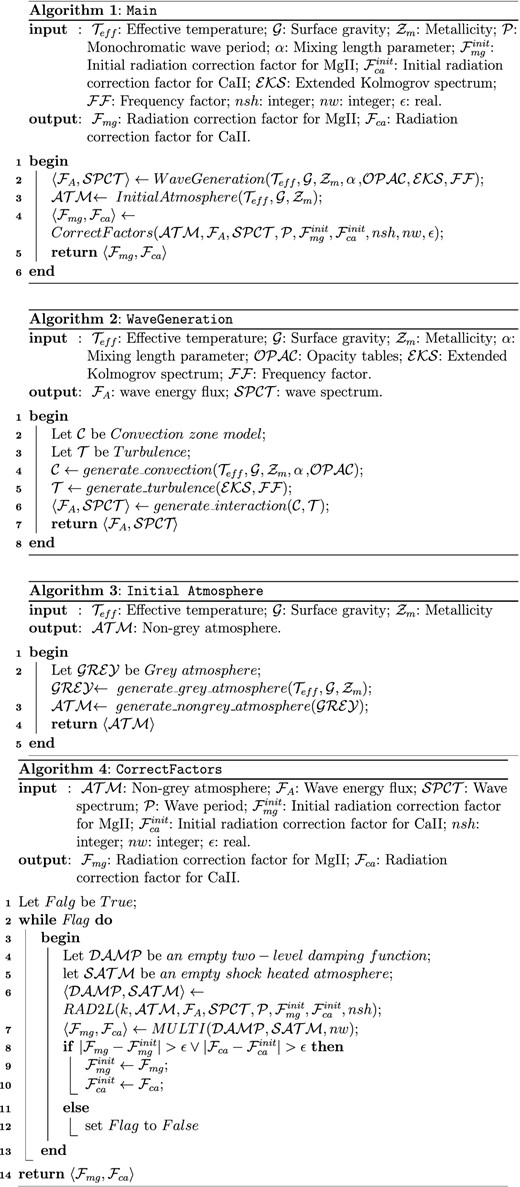
The algorithms used for the computation of the radiation correction factors. Credit: Diaa E. Fawzy 2015.
