


Abstract
Considering the contribution of emission from the host galaxies of gamma-ray bursts (GRBs) to radio afterglows, we investigate the effect of host galaxies on observations statistically. For the three types of event, i.e. low-luminosity, standard and high-luminosity GRBs, it is found that a tight correlation exists between the ratio of the radio flux (RRF) of the host galaxy to the total radio peak emission and the observational frequency. Towards lower frequencies, in particular, the contribution from the host increases significantly. The correlation can be used to obtain a useful estimate for the radio brightness of those host galaxies that only have very limited radio afterglow data. Using this prediction, we reconsidered the theoretical radio afterglow light curves for four kinds of event: high-luminosity, low-luminosity, standard and failed GRBs, taking into account the contribution from host galaxies and aiming to explore the detectability of these events by the Five-hundred-metre Aperture Spherical radio Telescope (FAST). Lying at a typical redshift of z = 1, most of the events can be detected easily by FAST. For the less fierce low-luminosity GRBs, their radio afterglows are not strong enough to exceed the sensitivity limit of FAST at such distances. However, since a large number of low-luminosity bursts actually happen very near to us, it is expected that FAST will still be able to detect many of them.
1 INTRODUCTION
Gamma-ray bursts (GRBs) are bright flashes of gamma-rays that happen randomly in the sky. They were serendipitously discovered in 1967 by the Vela satellites (Klebesadel, Strong & Olson 1973), but were poorly understood until 1997 February 28, when the first afterglow was detected (Groot et al. 1998). Subsequently, the counterpart of GRB 970508 was detected as the first afterglow in radio bands (Frail et al. 1997). The detection of afterglows makes it possible for us to obtain broad-band observational data, identify host galaxies and determine the redshifts of GRBs. The so-called fireball-shock model was developed to explain the main features of GRBs and their afterglows (Rees & Mészáros 1994; Piran 1999; Zhang 2007); the latter are generally believed to arise from interaction of the fireball with the surrounding interstellar medium (ISM) (Mészáros & Rees 1997; Piran 2000; Mészáros 2002).
According to the fireball-shock model (e.g. Mészáros 2002; Piran 2004; Zhang & Mészáros 2004; Zhang 2014), the outflow of a GRB interacts with the ISM to form an external shock. The shock accelerates electrons. At the same time, a fraction of the shock energy is transferred to the magnetic field. Afterglow emission arises from synchrotron radiation of these accelerated electrons, due to their interaction with the magnetic field. Within this framework, the main features of GRB afterglows can be explained well.
With more and more afterglows being detected, the study of GRBs has entered an era of full wavelengths (e.g. Gehrels & Razzaque 2013). However, according to Hancock, Gaensler & Murphy (2013), the detection rate of afterglows is only ∼30 per cent at radio wavelengths, although some authors have recently compiled several larger data sets (Chandra & Frail 2012; de Ugarte Postigo et al. 2012; Ghirlanda et al. 2013; Staley et al. 2013). Note that the search for radio afterglows is already at great depth (Chandra & Frail 2011). Another exclusive property of radio afterglows is their detection at high redshifts (Frail et al. 2006; Chandra et al. 2010). For example, there are about 350 GRBs with measured redshifts, of which ∼ 32 per cent are at redshifts z > 2, ∼7 per cent at z > 4 and ∼2 per cent at z > 6. The maximum redshift is 9.4 for GRB 090429B, indicating that GRBs are potentially powerful probes of the early Universe. In fact, the high luminosities of GRBs make them potentially detectable up to very high redshifts (Lamb & Reichart 2000). They may be observable with the current Very Large Array (VLA) up to z ∼ 30 at frequencies higher than ∼5 GHz (Ioka & Mészáros 2005; Mesler et al. 2014; Zhang et al. 2015).
China's Five-hundred-metre Aperture Spherical radio Telescope (FAST: Nan et al. 2011) is expected to be completed in 2016 September and will be the largest radio telescope in the world by then. FAST's receivers will cover both low (70 MHz–0.5 GHz) and middle (0.5–3 GHz) frequency ranges. Compared with the Arecibo radio telescope, FAST is expected to be three times more sensitive, with a tracking speed 10 times higher. Zhang et al. (2015, hereafter Paper I) estimated the exact sensitivity of FAST to GRB afterglows. They calculated the light curves of radio afterglows of typical low-luminosity, high-luminosity, failed and standard GRBs in different observational bands of FAST and found that almost all types of radio afterglow, except those from low-luminosity GRBs, could be detected by FAST up to z = 5. They also argued that FAST can detect radio afterglows at ν = 2.50 GHz up to z = 15 or even more. However, they did not consider the contribution from host galaxies of GRBs. In fact, the observed radio emission should include the afterglow component as well as the contribution from its host galaxy. In order to model the observed radio afterglows and evaluate the detectability of FAST more realistically, it is necessary to consider the contribution from the host galaxy.
In this study, we have collected a large sample of radio afterglows. We examine the relative contribution from the afterglows and their hosts based on our sample. For this purpose, we propose a useful method based on the flux ratio of the host to the afterglow to estimate radio flux density at a given frequency for different kinds of burst. Taking into account the contribution from the hosts, we then re-examine the detectability of FAST for those weak radio afterglows at very high redshifts. Our article is organized as follows. We briefly introduce the GRBs of our sample in Section 2. In Section 3, we present our statistical results on the ratio of host flux to radio peak flux (RRF). In Section 4, we present our theoretical radio afterglow light curves and evaluate the detectability of FAST. Our conclusions and discussion are given in Section 5.
2 SAMPLE
As of 2013 December, the number of observed radio afterglows is about 95, which is only ∼30 per cent of all GRBs with afterglows that have been observed. In practice, the observed radio emission should be composed of a GRB afterglow component and a contribution from the host galaxy. For GRB 980703, Berger, Kullarni & Frail (2001b) found that there is a constant component in the observed radio emission, which was interpreted as the first example of a host contribution to the afterglow (see also Frail et al. 2003). They argued that radio and submillimetre observations of GRB host galaxies will be very useful for studying the obscured star formation rate and the properties of starbursts at high redshifts. Berger et al. (2003a) pointed out that about 20 per cent of GRB host galaxies are ultraluminous (L > 1012 L⊙) and these can be utilized to probe a representative population of star-forming galaxies.
For bursts with detected radio afterglows, we collect the observational data of host galaxies together with their peak fluxes of radio afterglows at ν = 1.4–9.0 GHz. We obtain 50 GRBs in total and the data are listed in Table 1 . In our sample, there are 10 GRBs associated with supernovae (SNe). According to their isotropic energies, we classify the GRBs into three types: namely low-luminosity, standard and high-luminosity GRBs. The boundary energies for our classification are 1051 and 1053 erg, respectively. Six GRBs without known redshift are not included in the above three subsamples, but are treated as an independent subsample listed in Table 1.
Observational properties of 50 GRBs and their host galaxies in radio bands.
| GRB | |$E_{\rm iso}^a$| | |$T_{90}^a$| | za | Frequency | Host flux density | Peak flux densityb | Peak time | Referencesc | RRF |
|---|---|---|---|---|---|---|---|---|---|
| (1051 erg) | (s) | (GHz) | (μJy) | (μJy) | (days) | (per cent) | |||
| (1) | (2) | (3) | (4) | (5) | (6) | (7) | (8) | (9) | (10) |
| Low-luminosity GRBs | |||||||||
| 020903n | 0.023 | 13 | 0.250 | 1.43 | 43 ± 66 | 294 ± 91 | 36.73 | 28,9 | 14.6 ± 14.8 |
| 4.86 | 21 ± 34 | 782 ± 28 | 36.7 ± 1.3 | 28,9 | 2.7 ± 4.4 | ||||
| 8.46 | 190 ± 30 | 1058 ± 19 | 23.80 | 28,9 | 18.0 ± 2.9 | ||||
| 031203n | 0.115 | 30 | 0.105 | 1.43 | 254 ± 46h | 929 ± 60 | 65.5 ± 5.3 | 22,9 | 27.3 ± 5.3 |
| 4.86 | 393 ± 60 | 828 ± 28 | 58.4 ± 2.1 | 27,9 | 47.5 ± 7.4 | ||||
| 8.46 | 53 ± 52 | 724 ± 19 | 48 ± 1.3 | 27,9 | 7.3 ± 7.2 | ||||
| 050416An | 1.00 | 3 | 0.650 | 4.86 | 50.5 ± 41.8 | 485 ± 36 | 48.5 ± 3.5 | 30,9 | 10.4 ± 8.7 |
| 8.46 | 20 ± 51 | 373 ± 36 | 49 ± 3.6 | 30,9 | 7.3 ± 13.7 | ||||
| 060218n | 0.003 | 128 | 0.033 | 1.43 | 69.5 ± 69.5 | 198 ± 58 | 4.9 | 29,9 | 35.1 ± 36.6 |
| 4.86 | 32 ± 32 | 245 ± 50 | 3.8 ± 0.7 | 29,9 | 13.1 ± 13.3 | ||||
| 8.46 | 22.8 ± 20.5 | 471 ± 83 | 2 ± 0.3 | 29,9 | 4.8 ± 4.4 | ||||
| 100418An | 0.520 | 7 | 0.620 | 8.46 | 366 ± 53 | 1218 ± 12 | 47.6 ± 0.6 | 23,9 | 30.1 ± 4.4 |
| Standard GRBs | |||||||||
| 970508 | 7.10 | 14 | 0.835 | 1.43 | 100 ± 32 | 381 ± 19 | 179.1 ± 7.6 | 15,9 | 26.3 ± 8.5 |
| 4.86 | 104 ± 44 | 780 ± 13 | 57.6 ± 0.9 | 15,9 | 13.3 ± 5.6 | ||||
| 8.46 | 8 ± 19 | 958 ± 11 | 37.2 ± 0.4 | 17,9 | 0.8 ± 2.0 | ||||
| 980703 | 69.0 | 90 | 0.966 | 1.43 | 68 ± 6.6h | 263 ± 81 | 25.4 ± 5.5 | 3,9 | 25.9 ± 8.4 |
| 4.86 | 42.1 ± 8.6h | 1055 ± 30 | 9.1 ± 0.2 | 3,9 | 4.0 ± 0.8 | ||||
| 8.46 | 39.3 ± 4.9h | 1370 ± 30 | 10 ± 0.2 | 3,9 | 2.9 ± 0.4 | ||||
| 981226 | 5.90 | 20 | 1.11 | 8.46 | 12 ± 22.6 | 137 ± 34 | 8.2 ± 1.6 | 12,9 | 8.8 ± 1.7 |
| 000301C | 43.7 | 10 | 2.034 | 4.86 | 85 ± 33 | 240 ± 53 | 4.3 | 1,9 | 35.4 ± 15.8 |
| 8.46 | 18 ± 7h | 520 ± 24 | 14.1 ± 0.5 | 24,9 | 3.5 ± 1.4 | ||||
| 000418 | 75.1 | 30 | 1.119 | 1.43 | 48 ± 15h | 210 ± 180† | 16.56 | 4,2 | 22.9 ± 20.9 |
| 4.86 | 110 ± 52 | 897 ± 39 | 27 ± 1 | 4,9 | 12.3 ± 5.8 | ||||
| 8.46 | 37 ± 12h | 1085 ± 22 | 18.1 ± 0.3 | 4,9 | 3.4 ± 1.1 | ||||
| 010921 | 9.00 | 24 | 0.450 | 4.86 | 27 ± 25 | 161 ± 20 | 31.5 ± 3.3 | 17,9 | 16.8 ± 15.7 |
| 8.46 | 43.7 ± 21.3 | 229 ± 22 | 27.01 | 17,9 | 19.1 ± 9.5 | ||||
| 011211 | 63.0 | 400 | 2.140 | 8.46 | 24 ± 16 | 162 ± 13 | 13.2 ± 1.6 | 17,9 | 14.8 ± 9.9 |
| 020819B | 7.90 | 50 | 0.410 | 8.46 | 44.7 ± 23 | 291 ± 21 | 12.2 ± 1.1 | 20,9 | 15.4 ± 8.0 |
| 021004 | 38.0 | 50 | 2.330 | 4.86 | 78 ± 28 | 470 ± 26 | 32.2 ± 1.4 | 17,9 | 16.6 ± 6.0 |
| 8.46 | 59.4 ± 19.5 | 780 ± 23 | 18.7 ± 0.5 | 17,9 | 7.6 ± 2.5 | ||||
| 021211n | 11.0 | 8 | 1.010 | 8.46 | 12 ± 36 | 60 ± 28† | 8.85 | 11,11 | 20.0 ± 60.7 |
| 030329n | 18.0 | 63 | 0.169 | 1.43 | 450 ± 109 | 2232 ± 30 | 78.6 ± 2.1 | 5,9 | 20.3 ± 4.9 |
| 4.86 | 332 ± 51.7 | 10337 ± 33 | 32.9 ± 0.1 | 5,9 | 3.2 ± 0.5 | ||||
| 8.46 | 248 ± 48.2 | 19567 ± 28 | 17.3 ± 0.1 | 5,9 | 1.3 ± 0.3 | ||||
| 050824n | 1.50 | 23 | 0.830 | 8.46 | 36 ± 27 | 156 ± 34 | 7.2 | 17,9 | 23.1 ± 18.0 |
| 070612A | 9.12 | 369 | 0.617 | 4.86 | 222 ± 42.3 | 580 ± 20 | 140.3 ± 5.8 | 17,9 | 38.3 ± 7.4 |
| 8.46 | 68 ± 49 | 1028 ± 16 | 84.1 ± 2 | 17,9 | 6.6 ± 4.8 | ||||
| 071010B | 26.0 | 36 | 0.947 | 4.86 | 57 ± 60.4 | 227 ± 114 | 12.5 ± 4.4 | 17,9 | 25.1 ± 29.5 |
| 8.46 | 17 ± 47 | 341 ± 41 | 4.2 ± 0.5 | 17,9 | 5.0 ± 13.8 | ||||
| 090328 | 100 | 57 | 0.736 | 8.46 | 21 ± 64 | 686 ± 26 | 16.1 ± 0.7 | 7,9 | 3.1 ± 9.3 |
| 091020 | 45.6 | 39 | 1.710 | 8.46 | 90 ± 41.1 | 399 ± 21 | 10.9 ± 0.6 | 17,9 | 22.6 ± 10.4 |
| 100814A | 59.7 | 175 | 1.44 | 4.50 | 85 ± 27 | 496 ± 24 | 13 ± 1 | 17,9 | 17.1 ± 5.5 |
| 100901A | 17.8 | 439 | 1.408 | 4.50 | 75 ± 40 | 331 ± 30 | 4.9 | 17,9 | 22.7 ± 12.3 |
| High-luminosity GRBs | |||||||||
| 970828 | 296 | 147 | 0.958 | 1.43 | 14 ± 22 | 57 ± 51† | 208.1 | 10,10 | 24.6 ± 44.4 |
| 8.46 | 32 ± 20.5 | 144 ± 31 | 7.8 ± 1.8 | 10,9 | 22.2 ± 15.0 | ||||
| 980329 | 2100 | 58 | 2–3.9 | 1.43 | 38 ± 25.5 | 134 ± 43† | 113.54 | 32,32 | 28.4 ± 21.1 |
| 4.86 | 22 ± 37 | 171 ± 14 | 91.5 ± 11.3 | 32,9 | 12.9 ± 21.7 | ||||
| 8.46 | 13 ± 11 | 332 ± 11 | 33.5 ± 1.4 | 32,9 | 3.9 ± 3.3 | ||||
| 990123 | 2390 | 100 | 1.600 | 8.46 | 7.7 ± 11.1 | 260 ± 32† | 24.65 | 21,21 | 3.0 ± 4.3 |
| 990506 | 949 | 220 | 1.307 | 8.46 | 31 ± 27.6 | 581 ± 45† | 2.70 | 31,31 | 5.3 ± 4.8 |
| 991208n | 110 | 60 | 0.706 | 1.43 | 54.8 ± 44.4 | 263 ± 49 | 8.9 ± 1.8 | 18,9 | 20.8 ± 17.3 |
| 8.46 | 37.3 ± 25.8 | 1804 ± 24 | 7.8 ± 0.1 | 18,9 | 2.1 ± 1.4 | ||||
| 991216 | 675 | 25 | 1.020 | 8.46 | 20 ± 24.7 | 960 ± 67† | 1.49 | 13,13 | 2.1 ± 2.6 |
| 000210 | 200 | 10 | 0.850 | 8.46 | 18 ± 9h | 93 ± 21† | 8.59 | 4,25 | 19.4 ± 10.6 |
| 000911n | 880 | 500 | 1.059 | 4.86 | 10 ± 25 | 71 ± 23 | 11.1 | 26,9 | 14.1 ± 35.5 |
| 8.46 | 33.7 ± 25.2 | 263 ± 33 | 3.1 ± 0.3 | 26,9 | 12.8 ± 9.7 | ||||
| 000926 | 270 | 25 | 2.039 | 4.86 | 58 ± 41.5 | 460 ± 31 | 16.9 ± 1.5 | 19,9 | 12.6 ± 9.1 |
| 8.46 | 23 ± 9h | 629 ± 24 | 12.1 ± 0.5 | 24,9 | 3.7 ± 1.4 | ||||
| 010222 | 133 | 170 | 1.477 | 4.86 | 23 ± 8h | 144 ± 47 | 2.3 | 24,9 | 16.0 ± 7.6 |
| 8.46 | 38.8 ± 19.8 | 344 ± 39† | 1.35 | 17,17 | 11.3 ± 5.9 | ||||
| 020813 | 800 | 113 | 1.254 | 4.86 | 23 ± 42 | 349 ± 43† | 5.15 | 17,17 | 6.6 ± 12.1 |
| 8.46 | 30.8 ± 19.8 | 323 ± 39† | 1.24 | 17,17 | 9.5 ± 6.2 | ||||
| 030226 | 120 | 69 | 1.986 | 8.46 | 35 ± 18 | 171 ± 23 | 6.7 ± 1 | 17,17 | 20.5 ± 10.9 |
| 050603 | 500 | 12 | 2.821 | 8.46 | 79 ± 49 | 377 ± 53 | 14.1 ± 1.8 | 17,17 | 20.9 ± 13.3 |
| 050820A | 200 | 240 | 2.615 | 4.86 | 21 ± 51 | 256 ± 78† | 2.15 | 17,6 | 8.2 ± 20.1 |
| 8.46 | 76 ± 30 | 634 ± 62† | 0.93 | 6,6 | 12.0 ± 4.9 | ||||
| 050904 | 1300 | 174 | 6.290 | 8.46 | 13 ± 27 | 76 ± 14 | 35.3 ±1.5 | 16,9 | 17.1 ± 35.7 |
| 051022 | 630 | 200 | 0.809 | 8.46 | 41 ± 23 | 268 ± 32 | 5.2 ± 0.7 | 17,9 | 15.3 ± 8.8 |
| High-luminosity GRBs | |||||||||
| 070125 | 955 | 60 | 1.548 | 4.86 | 133 ± 21 | 308 ± 78 | 27.9 | 8,9 | 43.2 ± 12.9 |
| 8.46 | 64 ± 18 | 1028 ± 16 | 84.1 ± 2 | 8,9 | 6.2 ± 1.7 | ||||
| 071003 | 324 | 148 | 1.604 | 4.86 | 93 ± 52 | 224 ± 54 | 3.8 | 17,9 | 41.5 ± 25.3 |
| 8.46 | 109 ± 45 | 616 ± 57 | 6.5 ± 0.5 | 17,9 | 17.7 ± 7.5 | ||||
| 090323 | 4100 | 133 | 3.57 | 8.46 | 27 ± 38 | 243 ± 13 | 15.6 ± 1 | 7,9 | 11.1 ± 15.7 |
| 090902B | 3090 | … | 1.883 | 8.46 | 18 ± 16 | 84 ± 16 | 14.1 ± 2.6 | 7,9 | 21.4 ± 19.5 |
| 100414A | 779 | 26 | 1.368 | 8.46 | 20 ± 16 | 524 ± 19 | 8 ± 0.3 | 17,9 | 3.8 ± 3.1 |
| GRBs without known redshifts | |||||||||
| 980519 | … | 30 | … | 4.86 | 25 ± 27 | 330 ± 47 | 17.9 ± 2.4 | 14,9 | 7.6 ± 8.3 |
| 8.46 | 49 ± 28 | 205 ± 23 | 12.6 ± 1.3 | 14,9 | 23.9 ± 13.9 | ||||
| 001007 | … | 375 | … | 8.46 | 34 ± 61 | 222 ± 33 | 7.1 | 17,9 | 15.3 ± 27.6 |
| 001018 | … | 31 | … | 8.46 | 70 ± 23.3 | 590 ± 68 | 4.7 ± 0.6 | 17,9 | 11.9 ± 4.2 |
| 021206 | … | 20 | … | 4.86 | 58 ± 24 | 480 ± 69 | 7 ± 0.8 | 17,9 | 12.1 ± 5.3 |
| 041219A | … | 6 | … | 4.86 | 33 ± 48 | 473 ± 28 | 6.3 ± 0.9 | 17,9 | 7.0 ± 10.2 |
| 8.46 | 63 ± 42 | 518 ± 150† | 1.69 | 17,17 | 12.2 ± 8.8 | ||||
| 050713B | … | 125 | … | 4.86 | 44 ± 69 | 623 ± 53† | 21.01 | 17,17 | 7.1 ± 11.1 |
| 8.46 | 59 ± 40.5 | 373 ± 24 | 14.1 ± 0.9 | 17,9 | 15.8 ± 10.9 | ||||
aRefer to Chandra & Frail (2012).
bObserved radio peak flux density.
cReferences are in the following order: host radio flux density, radio peak flux density.
Abbreviations for the references are as follows: (1) Berger et al. (2000), (2) Berger et al. (2001a), (3) Berger et al. (2001b), (4) Berger et al. (2003a), (5) Berger et al. (2003c), (6) Cenko et al. (2006), (7) Cenko et al. (2011), (8) Chandra et al. (2008), (9) Chandra & Frail (2012), (10) Djorgovski et al. (2001), (11) Fox et al. (2003), (12) Frail et al. (1999), (13) Frail et al. (2000a), (14) Frail et al. (2000b), (15) Frail, Waxman & Kulkarni (2000), (16) Frail et al. (2006), (17) Frail & Chandra (2014, private communication), (18) Galama et al. (2003), (19) Harrison et al. (2001), (20) Jakobsson et al. (2005), (21) Kulkarni et al. (1999), (22) Michałowski et al. (2012), (23) Moin et al. (2013), (24) Perley & Perley (2013), (25) Piro et al. (2002), (26) Price et al. (2002), (27) Soderberg et al. (2004a), (28) Soderberg et al. (2004b), (29) Soderberg et al. (2006), (30) Soderberg et al. (2007), (31) Taylor et al. (2000), (32) Yost et al. (2002).
hHost flux densities have been reported in Berger et al. (2001b), Berger et al. (2003a), Michałowski et al. (2012) and Perley & Perley (2013).
nSN/GRB, i.e. SN-associated GRBs.
†These values are the maximum observed flux densities, which are taken as the observed peak flux densities.
In column 1 of Table 1, the GRB names are given. The isotropic energies Eiso, durations T90 in the observer's frame and redshift z are listed in columns 2, 3 and 4, respectively. Column 5 is the observational frequency. Column 6 tabulates the contribution from host galaxies. In this column, 10 radio fluxes for seven host galaxies have been reported directly in the literature. Other host fluxes are based on the assumption that the host flux density is constant at all stages of the afterglow, so that the host flux dominates at late times. We determine the host contribution only for those GRBs that were monitored in radio bands for a long period and with radio light curves that obviously become flat at the final stages.
Columns 7 and 8 tabulate the observed peak flux densities and the corresponding time of the peak. Most of the peak flux densities and the peak time are taken from Chandra & Frail (2012), who provided a sample with many events. They are determined by fitting the observed light curves. Meanwhile, for 13 GRBs, the peak flux densities of which are marked with daggers, the peak flux densities are simply the brightest measurements. This may cause the peak flux density to be somewhat underestimated, but not by enough to affect our results. The references of the host fluxes and the observed peak fluxes are listed in corresponding order in column 9. The data observed by Frail & Chandra have kindly been offered to us by the observers. It should be noted that, for some GRBs, other researchers may give different reports of host fluxes in the literature. For example, Berger et al. (2003b) and Soderberg et al. (2007) also reported flux densities for GRBs 020405 and 050416A, which are slightly different from the data in Table 1. However, these differences are generally not large enough to affect our results.
Using the RRF parameter, we can analyze the flux–flux correlation between host galaxies and GRB afterglows. It is interesting to note that our RRF analysis is completely independent of the distance (redshift) measurement.
3 RATIO OF RADIO FLUX DENSITIES
Considering the fact that most current GRB radio afterglows are observed at 1.43, 4.86 and 8.46 GHz, we use all data in these three bands except those without known redshifts in Table 1. In Fig. 1, we plot the observed host fluxes and peak fluxes versus frequency for different types of GRB. The data points are relatively scattered. We then calculate the mean values for the two fluxes at the three frequencies by assuming an equal weight for each data point on a logarithmic scale. Using the mean values of the host flux densities and the peak flux densities, we fit the correlations between the fluxes and the observational frequencies for low-luminosity, standard and high-luminosity GRBs, respectively. The results are also plotted in Fig. 1. Generally, the spectra of radio afterglows and host galaxies are usually considered to be a power-law function of frequency, so we select the power-law fit. In the three upper panels, the correlations are Fhost ∝ ν+0.04±0.02, Fhost ∝ ν−0.55±0.27 and Fhost ∝ ν+0.02±0.16 for low-luminosity, standard and high-luminosity GRBs, with the correlation coefficients and P-values (rejection possibilities) being (0.47, 0.0003), (0.60, 0.004) and (−0.95, 0.003) correspondingly. The three lower panels show that the observed peak fluxes are also correlated with the frequency as |$F_{\rm o,{\rm peak}}\propto \nu ^{+0.34\pm 0.13}$|, |$F_{\rm o,{\rm peak}}\propto \nu ^{+0.29\pm 0.18}$| and |$F_{\rm o,{\rm peak}}\propto \nu ^{+0.76\pm 0.24}$| for the three types of GRB, with the correlation coefficients and P-values being (0.80, 0.001), (0.61, 0.001) and (0.90, 0.002), respectively.
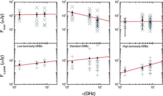
Observed host flux densities (upper panels) and peak flux densities (lower panels) as a function of the radio frequencies for low-luminosity (left), standard (middle) and high-luminosity GRBs (right) and our best fit to the observations. Filled circles with error bars are the mean values of the host flux densities at the corresponding frequency. Filled triangles with error bars are the mean values of the observed peak flux densities. The solid line in each panel represents our best fit to the observations. For the observational data and their references, please see Table 1 for details.
Theoretically, the radio flux density of a GRB afterglow can be simplified as a power-law function of time and frequency, say F ∝ tανβ (e.g. Sari, Piran & Narayan 1998; Wu et al. 2005; Paper I), where α and β are the temporal and spectral indices, respectively. Generally, the number density of the surrounding medium is assumed to depend on the shock radius as n ∝ R−k. Liang et al. (2013) and Yi, Wu & Dai (2013) argued that the k value should be in the range 0.4–1.4 for many GRBs, with a typical value of k ∼ 1. According to Wu et al. (2005), in the case of a homogenous ISM with k = 0, |$F_{\rm b,{\rm peak}}\propto \nu ^{0}$|. However, in the case of a typical stellar wind environment with k = 2, |$F_{\rm b,{\rm peak}}\propto \nu ^{1/3}$|, assuming the radio peak is caused when the synchrotron self-absorption frequency, νa, crosses the observational band. That is to say, the range of the power-law index for the |$F_{\rm b,{\rm peak}}$|–ν relation would be 0–1/3. Our fitting results are consistent with this range.
In our study, we average the original RRF values of the individual GRBs at a frequency to obtain a mean RRF value by assuming an equal weight for each observed data point. These mean values are then used in our final fitting process.

The best linear fits to RRF versus ν for low-luminosity, standard and high-luminosity GRBs and all GRBs as listed in Table 1. The observed frequencies ν are the three corresponding frequencies; in addition, one averaged data point at a frequency of 4.5 GHz is also included in the second panel. N in each panel is the number of original data points used to derive the mean observational values (solid circles).
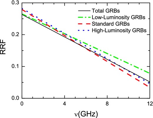
Comparison of the best linear fits of the RRF–ν correlation for different kinds of burst. Dash–dotted, dashed, dotted and solid lines represent the fits to low-luminosity, standard and high-luminosity GRBs and all GRBs, respectively.
In fact, according to the definition, RRF should be within the range 0–1. An RRF near 0 indicates that the afterglow component dominates the observed flux, while an RRF close to 1 indicates that the host flux is much larger than |$F_{\rm b,{\rm peak}}$|, which generally happens in low frequency ranges.
These RRF-predicted host fluxes can help us to subtract the potential radio background emission from a GRB source, so that the pure afterglow component can be identified, especially at lower frequencies. The RRF–ν correlation can also explain why low-frequency radio afterglows are usually difficult to detect, in contrast with the high-frequency case. According to the RRF–ν relation, radio fluxes are dominated by the host component at lower frequencies, as shown in Figs 1–3.
4 THEORETICAL RADIO AFTERGLOWS
According to equations (2)–(4), the host flux density depends on the observing frequency. Thus, we can use the RRF at a certain frequency to calculate the host flux density if the peak flux density of the radio afterglow is available. Here we use the theoretical peak flux density calculated from the fireball-shock model to estimate the host flux density. Taking into account the contribution from the host galaxy, we will then study the detectability of radio afterglows by FAST. Like Zhang et al. (2015) in Paper I, we also calculate the radio afterglow light curves for four kinds of GRB, i.e. standard, failed, high-luminosity and low-luminosity.
4.1 Dynamics
Here, we adopt the generic dynamical equations for beamed GRB outflows (e.g. Huang, Dai & Lu 1998, 1999a,b, 2000a,b) to calculate the radio afterglows of GRBs. The formulae of the dynamical model were widely applied in many studies, such as studies of overall afterglow modelling (Cheng & Wang 2003; Wu et al. 2004; Kong et al. 2009), rebrightening at multi-wavelengths (Dai et al. 2005; Kong et al. 2010; Xu & Huang 2010; Yu & Huang 2013; Hou et al. 2014) and the beaming effect (Huang, Dai & Lu 2000c; Wei & Lu 2002; Huang et al. 2003). These equations are valid in both ultrarelativistic and non-relativistic stages, thus they are especially convenient for calculating radio afterglows, which usually last for a very long period and may involve the Newtonian regime. In our calculations, the effects of electron cooling, lateral expansion and equal arrival time surfaces are included.
The parameters assumed in our calculations are listed in Table 3, where Eiso is the initial isotropic energy, γ0 is the initial bulk Lorentz factor, θ0 is the initial half-opening angle of the jet, θobs is the angle between the axis of the jet and the line of sight, n is the number density of surrounding ISM, p is the electron distribution index and ξe and |$\xi ^2_{B}$| are the energy fractions of electrons and magnetic field with respect to the total energy, respectively. The radiative efficiency ϵ is equal to 1 in the highly radiative case and 0 in the adiabatic case. The initial Lorentz factor and isotropic energy are evaluated differently for the four kinds of GRB, while the following common parameters are assumed to be universal: |$n=1\,\mbox{cm}^{-3}, p=2.5,\ \xi _{\rm e}=0.1,\ \xi ^2_{B}=0.001,\ \theta =0.1$| and θobs = 0. Meanwhile, we take ϵ = 0, since we are mainly considering late-time afterglows, which should be in the adiabatic regime.
Best-fitting parameters for the linear RRF–ν correlation.
| GRB type | Fitting results | |||
|---|---|---|---|---|
| a | b | Correlation coefficient | P-value | |
| Low-luminosity GRBs | 0.27 ± 0.02 | −0.016 ± 0.002 | 0.96 | 0.09 |
| Standard GRBs | 0.28 ± 0.02 | −0.020 ± 0.003 | 0.95 | 0.02 |
| High-luminosity GRBs | 0.28 ± 0.01 | −0.019 ± 0.002 | 0.98 | 0.06 |
| All GRBs | 0.26 ± 0.01 | −0.018 ± 0.002 | 0.98 | 0.07 |
Typical physical parameter values used in theoretical modelling of GRB afterglows.
| Source | Eiso | γ0 | θ0 | n | p | |$\xi ^2_{B}$| | ξe | ϵ | θobs |
|---|---|---|---|---|---|---|---|---|---|
| (erg) | (rad) | (cm−3) | (rad) | ||||||
| Standard GRBsa | 1.0 × 1052 | 300 | 0.10 | 1.0 | 2.5 | 1.0 × 10⁻³ | 0.10 | 0 | 0 |
| Failed GRBsa | 1.0 × 1052 | 30 | 0.10 | 1.0 | 2.5 | 1.0 × 10⁻³ | 0.10 | 0 | 0 |
| High-luminosity GRBsa | 1.0 × 1054 | 300 | 0.10 | 1.0 | 2.5 | 1.0 × 10⁻³ | 0.10 | 0 | 0 |
| Low-luminosity GRBsa | 1.0 × 1049 | 300 | 0.10 | 1.0 | 2.5 | 1.0 × 10⁻³ | 0.10 | 0 | 0 |
aRefer to Paper I.
Parameters of the nine sets of FAST receivers.
| No. | Bandsa | νca | Flux density limita |
|---|---|---|---|
| (GHz) | (GHz) | (μJy) | |
| 1 | 0.07–0.14 | 0.10 | 843.5 |
| 2 | 0.14–0.28 | 0.20 | 238.0 |
| 3 | 0.320–0.334 | 0.328 | 376.5 |
| 4 | 0.28–0.56 | 0.40 | 63.5 |
| 5 | 0.55–0.64 | 0.60 | 44.5 |
| 6 | 0.56–1.02 | 0.80 | 18.0 |
| 7 | 1.23–1.53 | 1.38 | 9.5 |
| 8 | 1.15–1.72 | 1.45 | 7.0 |
| 9 | 2.00–3.00 | 2.50 | 5.5 |
4.2 Numerical results
In order to make a comparative analysis with Paper I, we recalculate the radio afterglow light curves for four types of GRB according to FAST's nine passbands, assuming a typical redshift of z = 1.0. As in Paper I, we also adopt the limiting flux densities under an integral time of 30 min as the limiting sensitivity for FAST. The nine observational radio frequencies and corresponding 5σ limiting sensitivities of FAST receivers are listed in Table 4. The difference is that we now include the contribution from the host, whose flux is estimated from the linear RRF–ν correlation. Our numerical results are plotted in Fig. 4. We see that the host flux densities estimated from equations (2) and (4) are often significantly larger than the afterglow component at early and late times, which makes the total light curves much flatter than those in Paper I, which did not consider the host galaxy contribution. This would make the radio afterglows more difficult to identify, due to the influence of the relatively strong radio background.
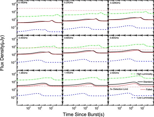
Predicted radio light curves within FAST's nine energy passbands for four kinds of GRB lying at z = 1.0 for the linear RRF–ν case. The thin solid, dash–dotted, dashed and thick solid lines correspond to failed, high-luminosity, low-luminosity and standard GRBs, respectively. The horizontal dotted lines represent the 5σ limiting sensivities of FAST for a 30-minute integration time (Paper I). Note that the host flux densities predicted by the linear RRF–ν correlation have been added in these light curves.
According to Fig. 4, standard GRBs could be observed by FAST at frequencies ν > 0.80 GHz, although at ν = 0.80 GHz the predicted peak flux density is 19.6 μJy and the 5σ detection limit of FAST for a 30-minute integration time is 18.0 μJy. Note that high-luminosity GRBs have the brightest radio afterglows, so that they can be detected easily in most bands with ν > 0.40 GHz. At ν = 0.40 GHz, FAST can detect high-luminosity GRBs from ∼0.1–1270 d.
An interesting phenomenon displayed in Fig. 4 is that the radio afterglows of standard and failed bursts are very different at frequency ν ≥ 1.38 GHz. The reason is that the initial bulk Lorentz factor of failed GRBs is about ten times smaller than that of standard ones. A lower Lorentz factor leads to a lower flux density at early times as well as a lower peak flux density. However, the late-time afterglow depends mainly on the intrinsic energy of the jet, so the light curves differ from each other only slightly at late stages, especially at low frequencies (Wu et al. 2004). The radio emission can be detected from ∼4000 s to ∼58 d at ν = 1.38 GHz. At ν ≥ 1.45 GHz, FAST can potentially detect very early radio emission.
Radio afterglows of low-luminosity bursts are the weakest ones in each panel of Fig. 4. For example, the strongest peak flux is only 0.14 μJy at ν = 2.50 GHz. According to our calculations, FAST can hardly detect any radio afterglows of low-luminosity GRBs at redshift z = 1. However, many low-luminosity GRBs are likely to happen very near to us, thus they can also be observed by FAST. A good example is the low-luminosity GRB 980425 (z = 0.0085). At such a small distance, its radio brightness is very high. As shown in Fig. 5, radio afterglows of low-luminosity GRBs can be detected by FAST at a redshift of z < 0.1. Fan, Piran & Xu (2006) argued that such underluminous GRBs with less kinetic energy might be very common. We expect that many more low-luminosity GRBs will be detected by FAST in the future.
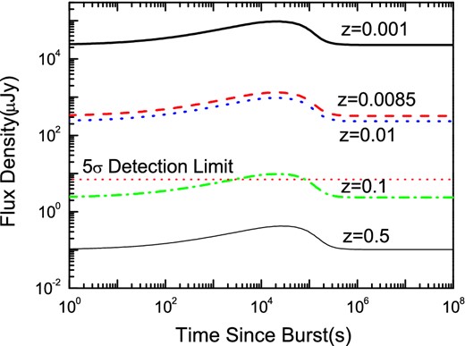
Predicted radio light curves of low-luminosity GRBs at 1.45 GHz for the linear RRF–ν case. The redshifts for the thick solid, dashed, dotted, dash–dotted and thin solid lines are z = 0.001, 0.0085 (the redshift of GRB 980425), 0.01, 0.1 and 0.5, respectively. The horizontal dotted line represents the 5σ limiting sensivity of FAST for a 30-minute integration time (Paper I). Note that the host flux densities predicted by the linear RRF–ν correlation have been added in these light curves.
5 DISCUSSION AND CONCLUSIONS
In this study, we investigate statistically the connection between host fluxes and peak afterglow fluxes in radio bands. The observed GRBs are classified into three types: low-luminosity, standard and high-luminosity. It is found that there is an anticorrelation between the RRF and the observational frequency. At a higher frequency, the corresponding RRF is smaller. This could be due to more significant self-absorption at longer wavelengths (Rybicki & Lightman 1979). Based on this correlation, the host flux densities at different radio frequencies can be estimated. This RRF prediction is especially helpful for those GRBs for which radio afterglow data are very limited. Meanwhile, we also reconsidered the capability of detecting GRBs with FAST. FAST has nine energy channels in its first phase, ranging from 0.10–2.50 GHz (Nan et al. 2011). It will operate mainly in a relatively low frequency range. Our results show that, at a typical redshift of z = 1.0, the radio emission of standard GRBs can be detected well by FAST at ν ≥ 1.38 GHz. Although FAST can barely detect radio afterglows from low-luminosity GRBs located at this redshift, we expect that a large population of low-luminosity GRBs could still be observable, since many such events may actually happen much nearer to us.
The host galaxies of long GRBs can help to reveal the environments and populations of unusual GRB progenitors (Levesque 2014). Berger (2014) argued that the properties of short GRB hosts will hint at the redshift distribution and shed light on the age distribution of the progenitors. Berger et al. (2001b) proposed that if more host galaxies are detected and studied in detail in the radio and submillimeter/FIR wavelengths then we will be able to address a large number of issues pertaining not only to the bursts themselves but also to the characteristics of galaxies at high redshifts. This will lead to a thorough understanding of GRB trigger mechanisms and host environments. Unfortunately, the detection rate of afterglows in radio bands is only ∼30 per cent, which is significantly lower than that of optical and X-ray afterglows.
In Paper I, the peak flux density versus the peak frequency for the above-mentioned four types of GRB at different redshifts was plotted theoretically. It was shown that the radio flux density F is a power-law function, F ∝ ν2 (e.g. Sari, Piran & Narayan 1998; Wu et al. 2005), if the observing frequency ν is below the synchrotron self-absorption frequency νssa. The dependence of the radio afterglow light curves on various parameters has been investigated by some authors, such as Chandra & Frail (2012). They found that the radio afterglow is relatively bright when the ISM density is between n = 1 and 10 cm−3. This may explain why some GRBs bright in X-ray/optical bands are dim in radio bands. Also, the radio brightness depends strongly on the intrinsic energy of the outflow, so there is evidently a close relationship between the detectability of the radio afterglow and the intrinsic physical parameters of the GRB (Zhang et al., in preparation).
We thank the anonymous referee for valuable comments and suggestions that led to an overall improvement of this study. We acknowledge D. A. Frail and P. Chandra for kindly offering their invaluable radio afterglow data to us. We are thankful to B. Zhang, B.B. Zhang and Y. Z. Fan for helpful discussions. This work is partly supported by the National Basic Research Program of China (973 Program, Grant No. 2014CB845800) and the National Natural Science Foundation of China (Grant Nos 11263002, 11473012 and 11322328). XFW and DL acknowledge support by the Strategic Priority Research Program ‘The Emergence of Cosmological Structures’ (Grant No. XDB09000000) of the Chinese Academy of Sciences. SWK acknowledges support by China Postdoctoral Science Foundation under grant 2012M520382. HYC was supported by BK21 Plus of the National Research Foundation of Korea and a National Research Foundation of Korea Grant funded by the Korean government (NRF-2013K2A2A2000525).
