


Abstract
Measured in situ, the particle velocity distributions in the solar wind plasma reveal two distinct components: a Maxwellian (thermal) core, and a less dense but hotter suprathermal halo with a power-law distribution described by Lorentzian/Kappa distribution function. Despite this evidence, the existing attempts to parametrize anisotropic distributions and the resulting wave instabilities are limited to idealized models, which either ignore the suprathermal populations, or minimize the core, assuming it is cold. Here, a more realistic approach is identified, combining an isotropic Maxwellian core and an anisotropic bi-Kappa halo. This model is relevant at large heliocentric distances and for the slow winds, when the field-aligned strahl is less pronounced and kinetic energy densities in the core and halo are comparable. A comparative study with the cold-core-based model is performed on the electron whistler–cyclotron instability driven by the anisotropic halo. Derived exactly numerically, the instability thresholds and growth rates confirm the expectation that cyclotron instabilities are inhibited by the core thermal spread. This effect is enhanced by the increase of the halo–core relative density with heliocentric distance, suggesting that local conditions for this instability to develop at large radial distances in the solar wind are less favourable than predicted before.
1 INTRODUCTION
Space plasmas are turbulent media pervaded by electromagnetic (EM) fields on a wide range of time and length-scales, from the inertial frequencies below the ion gyrofrequency (Zimbardo et al. 2010; Bruno & Carbone 2013) to the dissipation scale of electron frequencies (Lengyel-Frey et al. 1996; Briand 2009). Because these plasmas are hot and dilute, binary collisions between particles are not efficient. The main role must be played by the EM fields which are expected to control the plasma thermodynamics as well as the transport of particles and energy. Thus, an important fraction of EM turbulence can be generated locally by the instabilities driven by the kinetic anisotropy of plasma particles, like beams of electrons and ions, or the temperature anisotropy (Gary 1993).
Direct in situ measurements in the solar wind and planetary magnetospheres confirm the existence of such sources of free energy in the distributions of all species of plasma particles (Marsch 2006; Samsonov et al. 2007; Stverak et al. 2008). The observed velocity (or energy) distributions consist of two distinct components: the main core population, rather isotropic and almost Maxwellian, and a less dense, but hotter and highly anisotropic halo. The halo populations reside in the high-energy (suprathermal) tails of the distributions, which are well described by the Kappa power laws (Maksimovic et al. 2005; Stverak et al. 2009). A third component, viz. strahl (beaming) population, becomes more apparent in the fast solar wind (as an additional drifting component of the halo), moving outwards from the Sun with a finite angular width, and maximum intensity in the magnetic field direction.
Despite this observational evidence, the present attempts to parametrize the observed anisotropic distributions and the resulting plasma wave instabilities are limited to idealized models of velocity distribution functions (VDFs): (a) the core is considered to be of Maxwellian-type and suprathermal populations are completely ignored (see the textbook of Gary 1993). This model can be of particular interest at low heliocentric distances R < 1 au, where the high-density core hardly dominates the more dilute halo component (Maksimovic et al. 2005; Stverak et al. 2009), and when the core anisotropy can manifest itself in either parallel (Tc, ∥ > Tc, ⊥) or perpendicular (Tc, ∥ < Tc, ⊥) direction with respect to the magnetic field (Marsch 2012); (b) the role of the core is minimized, assuming this component to be cold, and suprathermal tails are modelled with a Kappa distribution function (Xiao et al. 2006, 2007); (c) both the core and halo populations are incorporated in a single global Kappa (see the reviews by Hellberg, Mace & Cattaert 2005; Pierrard & Lazar 2010) that is nearly Maxwellian at lower energies, and decreases smoothly as power law at high speeds; (d) a combination of two Maxwellians is considered, one for the core and another one, less dense but hotter for the suprathermal tails.1
Implying a reduced number of (macroscopic) plasma parameters used to describe the moments of the distribution (as well as their time and space evolution), these simplified models are convenient computationally, but they can omit important kinetic effects. For instance, it can be completely unrealistic to ignore the anisotropic halo, when this is the main trigger of the kinetic instabilities, or to neglect the thermal spread in the core populations that can reduce the free energy or interact with the resulting field fluctuations. The core component is hot enough even at large heliocentric distances R > 1 au, where the Ulysses observations (ftp://www.rssd.esa.int/pub/ulysses/data/swoops/) indicate for the electron core temperature values exceeding 105 K at 1.3 au, or 104 K at 5 au. Moreover, using the same observational data, we can estimate the electron beta parameter, which compares the kinetic energy of the plasma particles with the magnetic field energy, and find that kinetic energies stored by the core and halo populations are often comparable (see Section 3 below) even in the slow solar wind, when the halo is not enhanced by fast flows.
Within this paper, we propose a realistic parametrization of the kinetic anisotropies indicated by the observations in space plasmas. Although the stability analysis implies additional complications, our goals are to identify the conditions under which the realistic (less-idealized) models are approachable, and compare their dispersion and stability properties with the idealized models. Present analysis starts in Section 2 by introducing a general model for the gyrotropic velocity distributions of plasma particles. It is called general because this model reproduces fairly well all the main features of the VDFs observed in space plasmas (Maksimovic et al. 2005; Stverak et al. 2009). Thus, it can describe the principal components of the distribution and their (temperature) anisotropy: the core is modelled by a bi-Maxwellian and the halo by a bi-Kappa. A drifting strahl can also be previewed in the general model in order to cover conditions in the fast wind, or more energetic events (like coronal mass ejections (CMEs) or interplanetary shocks, when double-strahls or counterstreams are observed both parallel and antiparallel to the magnetic field). In the presence of these sources of free energy, the general model provides a realistic interpretation, but the high number of parameters involved yields a wide variety of cases to be studied and makes their analysis not a trivial task. However, under certain circumstances (more or less) indicated by the observations, the number of these parameters can be reduced. The existing attempts to examine realistic models are limited to isotropic VDFs with two distinct populations of electrons, a Maxwellian core and a distinct suprathermal Kappa component (Mace, Amery & Hellberg 1999). Kinetic anisotropies and the resulting instabilities have only been approached using the idealized models enumerated above.
Here, we find computationally tractable a less-idealized model of anisotropic distributions, which combines a nearly isotropic core of finite (Maxwellian) thermal spread (Tc ≠ 0), and an anisotropic halo modelled by a bi-Kappa distribution function. Emerging from the general (non-drifting) model, this new approach is relevant for the observations revealing thermal cores less anisotropic than the hotter and variably skewed halo populations (Marsch 2006). It may be of particular importance at large heliocentric distances R > 1 au (Ulysses observations), where the halo relative density is significantly increased at the expense of the strahl relative density (Maksimovic et al. 2005; Stverak et al. 2009). In Section 3, we apply this model to describe the instability of EM electron–cyclotron (EMEC) modes and compare with the simplified approaches. These modes are frequently associated with the small-scale turbulence observed in the solar wind (Lengyel-Frey et al. 1996; Lin et al. 1998) and planetary magnetospheres (Scarf et al. 1982; Zhang, Matsumoto & Kojima 1998), and their instability conditions were extensively studied, but only using simplified models of VDFs, viz. models (a)–(d) discussed above (Gary & Madland 1985; Gary & Wang 1996; Mace 1998; Xiao et al. 2006, 2007; Mace & Sydora 2010; Lazar, Poedts & Schlickeiser 2011; Lazar, Poedts & Michno 2013).
2 MODEL OF THE DISTRIBUTION
3 THE INSTABILITY OF EMEC MODES
In order to investigate the effects introduced by the thermal spread of plasma particles from the core, here we consider the particular case of the EM electron whistler–cyclotron modes, also known as the EMEC modes. Linear theory predicts a destabilization of these modes for an excess of the electron temperature in perpendicular direction (T⊥ > T∥), and when the distribution function decreases monotonically with increasing speed of the electrons (like our new model introduced in Section 2), the parallel-propagating modes are the most unstable (Kennel & Petschek 1966).
3.1 Dispersion relations
3.2 Parameters estimates from observations
We use the Ulysses/SWOOPS electron data, e.g. densities and temperatures provided distinctively for the core and halo populations, and the corresponding Ulysses 1-h averaged measurements of magnetic field and solar wind bulk speed data for the period 1994–2004. In Table 1, a number of 20 time intervals are identified from the periods of slow winds with flow speeds sufficiently low, i.e. VSW < 360 km s−1), such that any strahl component associated with the fast winds is not significantly apparent in the distributions. Moreover, these intervals are selected such that there is no CME event to interfere, as long as it is known that distributions can be markedly affected by additional counterstreaming populations during CMEs, and a plasma beta less than 0.2 is a specific signature of the CMEs (Lepping et al. 2003; Foullon et al. 2007). The CMEs catalogues of Ebert et al. (2009) and Du, Zuo & Zhang (2010) were considered in our selection. In these intervals of slow wind, the Ulysses observations cover a wide range of heliocentric distances, i.e. 1.34 au ≤ R ≤ 5.41 au, and heliolatitudes, i.e. −80° ≤ Lat ≤+58°, which are indicated in Table 1 for the corresponding day of year (DOY).
Selected time intervals of slow solar wind (VSW ≤ 360 km s−1), identified in the Ulysses data between 1995 and 2004.
| Start | End | |||
|---|---|---|---|---|
| Year | DOY-hr:min | DOY-hr:min | R(au) | Lat(deg) |
| 1995 | 70-9:50.4 | 74-13:55.2 | 1.34 | 5.1 |
| 1997 | 197-12:57.6 | 198-9:50.4 | 5.18 | 7.7 |
| 1997 | 267-6:57.6 | 271-18:57.6 | 5.28 | 4.1 |
| 1997 | 346-12:57.6 | 347-19:55.2 | 5.36 | 0.1 |
| 1998 | 15-0:0 | 21-6:57.6 | 5.38 | −1.6 |
| 1998 | 62-12:57.6 | 63-16:48 | 5.40 | −3.9 |
| 1998 | 88-8:52.8 | 89-7:55.2 | 5.41 | −5.2 |
| 1999 | 91-20:52.8 | 92-14:52.8 | 5.03 | −23.9 |
| 1999 | 211-12:57.6 | 214-23:45.6 | 4.72 | −30.9 |
| 1999 | 278-13:55.2 | 278-22:48 | 4.51 | −35.4 |
| 2000 | 182-0:43.2 | 190-7:55.2 | 3.26 | −60.3 |
| 2000 | 202-13:55.2 | 204-7:40.8 | 3.14 | −62.9 |
| 2000 | 276-0:0 | 278-6:57.6 | 2.67 | −74.1 |
| 2000 | 324-12:0 | 332-16:48 | 2.34 | −80 |
| 2001 | 6-0:43.2 | 18-13:55.2 | 2.00 | −73.4 |
| 2001 | 122-1:55.2 | 123-9:50.4 | 1.36 | −11.2 |
| 2001 | 219-3:50.4 | 220-13:55.2 | 1.58 | 58.5 |
| 2002 | 127-1:55.2 | 130-13:55.2 | 3.37 | 45.8 |
| 2002 | 298-18:0 | 298-7:40.8 | 4.20 | 29.1 |
| 2004 | 133-6:0 | 134-19:55.2 | 5.40 | −4 |
The halo–core relative density η = nh/nc determined for these intervals is displayed in Fig. 1 as a function of plasma beta for the core population (top panel), and the halo population (bottom panel). The relative density is in general very small, taking values in the interval 0.003 < η < 0.1. The core populations are mainly concentrated in the range of 0.3 < βc < 5, while the halo populations are in the range of 0.05 < βh < 1 (marked with grey shading in Fig. 1, bottom panel). Lower counts of halo populations extend to lower values down to βh ≥ 0.01 and to higher values of this parameter, up to βh ≤ 10. The data alignment along the dotted line in Fig. 1, bottom panel, suggests a direct dependence of the relative halo–core density (η) on the kinetic energy density and implicitly on the plasma beta of the halo populations (βh). At low βh ≤ 0.05, the number of counts are therefore expected to be enhanced by measurements at lower heliocentric distances R < 1 au, where the halo component exhibits lower densities (Stverak et al. 2009). In the same way, the number of events at large βh > 1 is enhanced by an increase in density of the halo populations with radial distance.

The estimates in Fig. 1 are not intended to an extend observational analysis, but to characterize the core and halo components and establish realistic conditions for the EMEC instability in the solar wind. For the core plasma beta, we chose the most probable value βc = 1.0, and for the halo–core relative density, we consider two values η = 0.01 and 0.05 found to be relevant for a large enough number of events. The instability thresholds are determined in the next section for an extended range of the halo beta 0.01 ≤ βh, ∥ ≤ 10.
3.3 The instability thresholds
Analytically, the unstable solutions of the dispersion relations (16) and (17) can be described only in the limits of large (|f| ≫ 1) or small (|f| ≪ 1) arguments of the plasma dispersion functions, e.g. in equations (12) and (14). But these limits do not cover the resonant regimes of the wave–particle interactions, i.e. |f| ∼ 1, which are particularly important for the cyclotron modes. In order to avoid these limitations, the instability thresholds and the unstable wave solutions are derived exactly numerically.
Let us first discuss the instability thresholds. The wave solutions are unstable, i.e. ℑ(ω) ≡ γ > 0, only for plasma parameters satisfying the instability condition, i.e. for sufficiently high-temperature anisotropy, exceeding the instability threshold. For the cyclotron modes, it is possible to describe the instability condition strictly depending on the plasma parameters, only evaluating the instability thresholds associated with a non-zero value of the maximum growth rate γm ≠ 0 (Gary & Wang 1996). These values are usually chosen to be very low, e.g. γm/|Ωe| ≪ 1, close to the marginal stability γm = 0. An exact analytical form of the marginal stability condition strictly depending on plasma parameters cannot be established for the cyclotron modes.
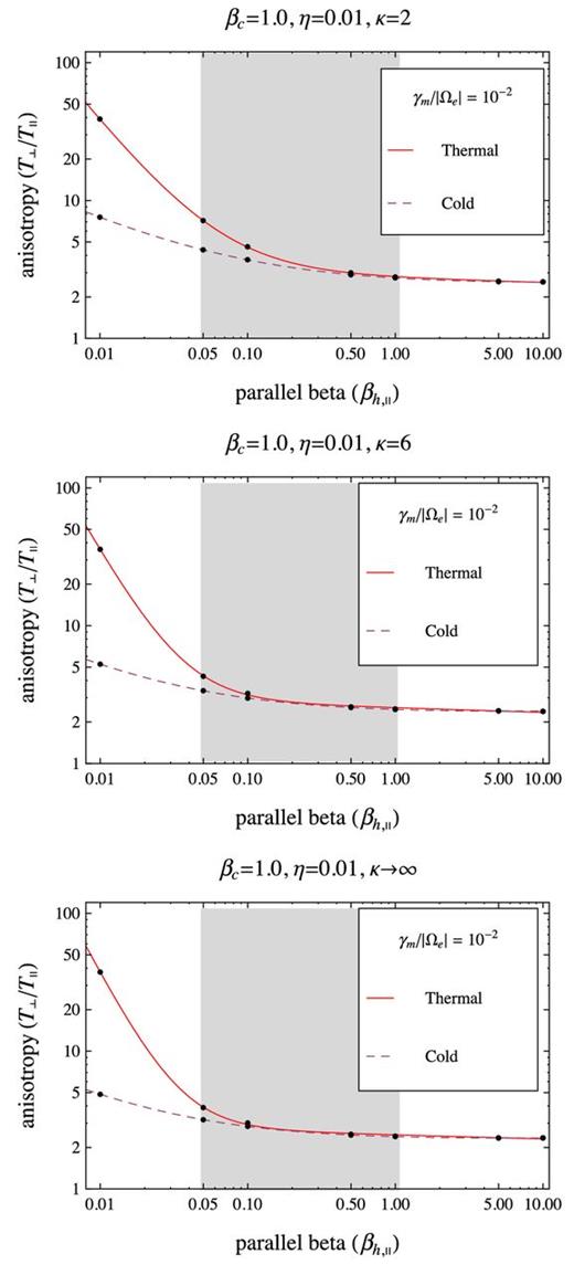
The anisotropy thresholds for γm/|Ωe| = 10−2 as provided by a thermal core model with βc = 1 (solid lines), and a cold-core model (dashed lines). Comparison is extended for three distinct Kappa models for the halo with the same η = 0.01, but different κ = 2 (top), 6 (middle) and κ → ∞ (bottom).
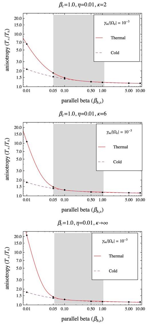
The same as in Fig. 2 but for γm/|Ωe| = 10−3.
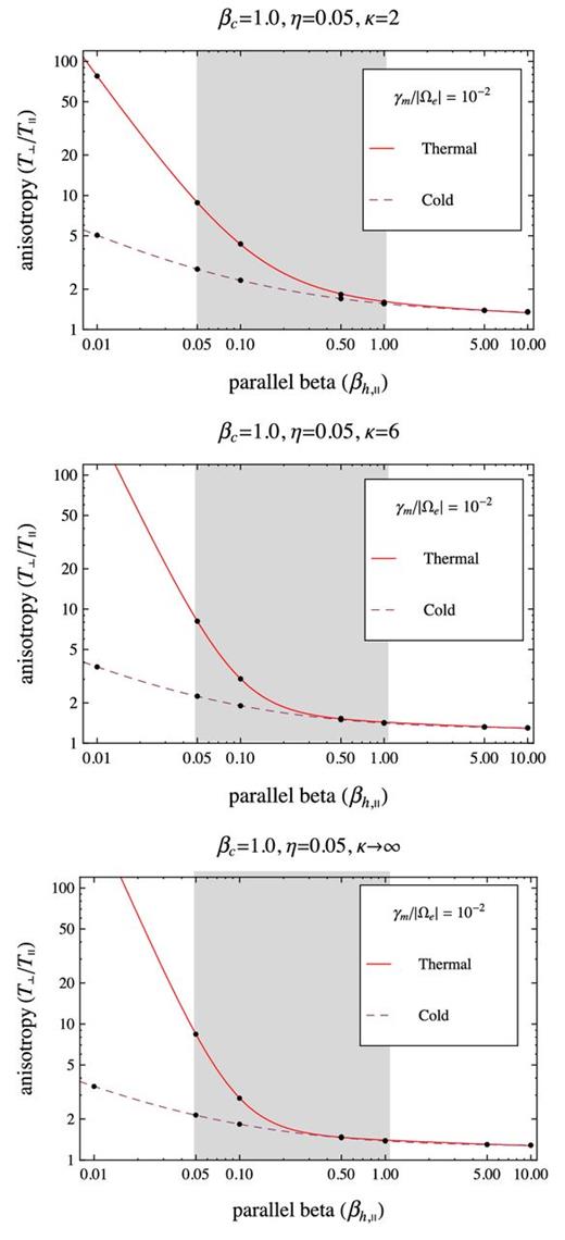
The anisotropy thresholds for γm/|Ωe| = 10−2 as provided by a thermal core model with βc = 1 (solid lines), and a cold-core model (dashed lines). Comparison is extended for three distinct Kappa models for the halo with the same η = 0.05, but different κ = 2 (top), 6 (middle) and κ → ∞ (bottom).
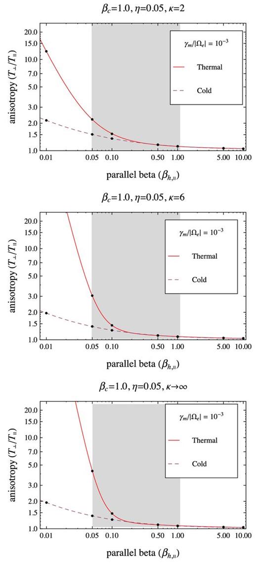
The same as in Fig. 4 but for γm/|Ωe| = 10−3.
Comparing the two models in Figs 2– 5, we find that anisotropy thresholds are increased by the finite thermal spread in the core, and this effect becomes more significant at lower values of the halo–plasma beta parameter βh < 0.5. The difference between these two models becomes even more pronounced at higher values of the halo–core relative density. The interval of halo–plasma beta values 0.05 ≤ βh ≤ 1 found relevant for our selection of slow wind events (see Fig. 1) is again marked with grey shading in Figs 2–5. The instability thresholds are also compared for different values of the kappa index, i.e. κ = 2, 6, ∞, enabling us to understand the influence of suprathermal (halo) populations, but also to contrast with the simplified model of two Maxwellians (see the Introduction). For all cases studied in Figs 2–5 with a cold-core model, the instability thresholds exhibit the same tendency of increasing with decreasing κ → 2, indicating that instability is inhibited by the suprathermal populations.2 In the approach with a thermal core, suprathermals have the same influence, but only for sufficiently high values of the halo beta parameter. At lower halo betas, and especially for high values of the relative halo–core density, e.g. Figs 4 and 5, the effect is opposite diminishing the instability thresholds with increasing κ → 2. Indeed, the contrast we found between the thermal and cold-core models does not change uniformly with the presence of suprathermal population, but it highly depends on the relative halo–core density. Thus, for a low η = 0.01 (in Figs 2 and 3), the difference between the instability thresholds provided by the thermal and cold-core models is more important at low κ → 2, and restraints to low betas βh, ∥ < 0.1. For a higher η = 0.05 (in Figs 4 and 5), the inhibiting effect of the thermal core extends to even higher betas βh, ∥ < 1, and becomes more significant at high values of the power index κ → ∞.
3.4 The unstable solutions
The main conclusion that follows from the analysis above is that EMEC instability is inhibited by the thermal spread of the core by increasing the instability thresholds. However, a complete picture on how the wave frequency and the range of the unstable wavenumbers are affected can be obtained only by investigating the unstable solutions. In order to do that, we consider each of the cases identified above.
3.4.1 Low-βh, ∥ regime
The unstable solutions displayed in Figs 6 –9 are derived for a low value of the halo beta parameter βh, ∥ = 0.05 and a sufficiently high value of the temperature anisotropy, A = T⊥/T∥ = 4, such that the growth rates are expected to display maxima in the vicinity of the higher thresholds (γm = 10−2|Ωe|) discussed above. We keep the plotting style, as to have the solutions provided by the thermal core model, i.e. dispersion relation (16), displayed with solid lines, while those derived from the cold-core model, i.e. dispersion relation (17), plotted with dashed lines. The growth rates plotted in Figs 6 and 7 confirm the inhibiting effect of the thermal core populations on the EMEC instability by lowering their maximum values by comparison to the cold-core model. With increasing the relative density η of the anisotropic halo populations, this effect becomes more pronounced. In addition, the unstable wavenumbers undergo a significant restraint to small values for both levels of η = 0.01, 0.05. The wave frequency of these growing modes, ωr ≡ ℜ(ω), is displayed in Figs 8 and 9, showing the same inhibiting effect, but with a less important decrease of its value in the range of unstable wavenumbers.
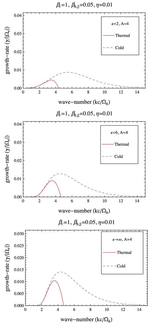
Growth rates of the whistler instability as provided by our models with a thermal core with βc = 1 (solid red lines), and a cold core (dashed lines). Comparison is extended for three halo models with the same η = 0.01, βh, ∥ = 0.05 and A = 4, but different κ = 2 (top), κ = 6 (middle) and κ → ∞ (bottom).

The same as in Fig. 6 but for a higher η = 0.05. For large κ → ∞, the instability is (almost) stabilized by the hot core.
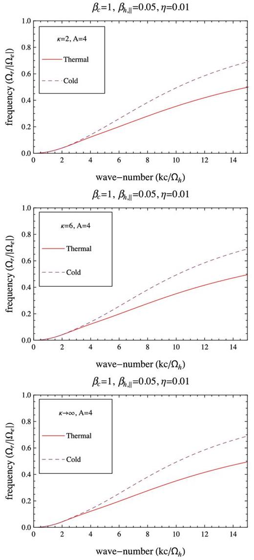
Frequency of the unstable modes in Fig. 6.
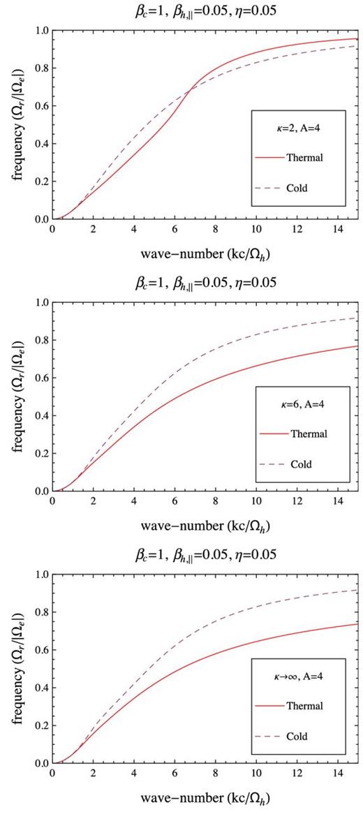
Frequency of the unstable modes in Fig. 7.
The unstable solutions are also compared for different values of the power index, i.e. κ = 2, 6, ∞. It is important to understand the influence of suprathermal populations because not only the halo density is enhanced with the radial heliographic distance (R), but also the suprathermal populations as the observational analysis indicate a decrease of the power-law index down to very low values 2 ≤ κ ≤ 3 at R ≥ 2 au (Stverak et al. 2009). In this case, the influence of suprathermals is highly dependent on the level of η. For a low η = 0.01, the growth rates are diminished with decreasing κ → 2 for both the cold-core and thermal-core models. For a higher η = 0.05, the growth rates exhibit the same behaviour for the cold-core model, but the growth rates provided by a thermal-core approach are enhanced by an increase of suprathermal population (decreasing κ → 2). In the limit of very large κ → ∞, our model reduces to the more idealized model of two Maxwellians, and the instability is stabilized by the hot core if η is sufficiently high. The effect of suprathermals on the unstable wavenumbers and frequency is not noticeable, with an exception at high η = 0.05 and low κ = 2, when the wave frequency from the thermal-core model overcomes that from the cold-core approach. But this effect restrains only to the large wavenumbers which are not relevant for the instability.
3.4.2 High-βh, ∥ regime
The unstable solutions presented in Figs 10 –13 are derived for a higher value of the halo beta parameter βh, ∥ = 0.3 and a lower value of the temperature anisotropy, A = T⊥/T∥ = 1.4, such that the growth rates are again expected to display maxima in the vicinity of the thresholds (high halo betas) discussed in Section 3.3. Due to the hot core, the growth rates exhibit the same inhibiting effect, but the difference between their maxima is much lower than found in the low-βh, ∥ regime. Less significant are also the restraining effect on the unstable wavenumbers, and the inhibiting effect on the wave-frequency (Figs 11–12). But the inhibiting effect remains more pronounced for a higher η. In this case, the suprathermals have an uniform effect, the instability being always inhibited with decreasing κ → 2.
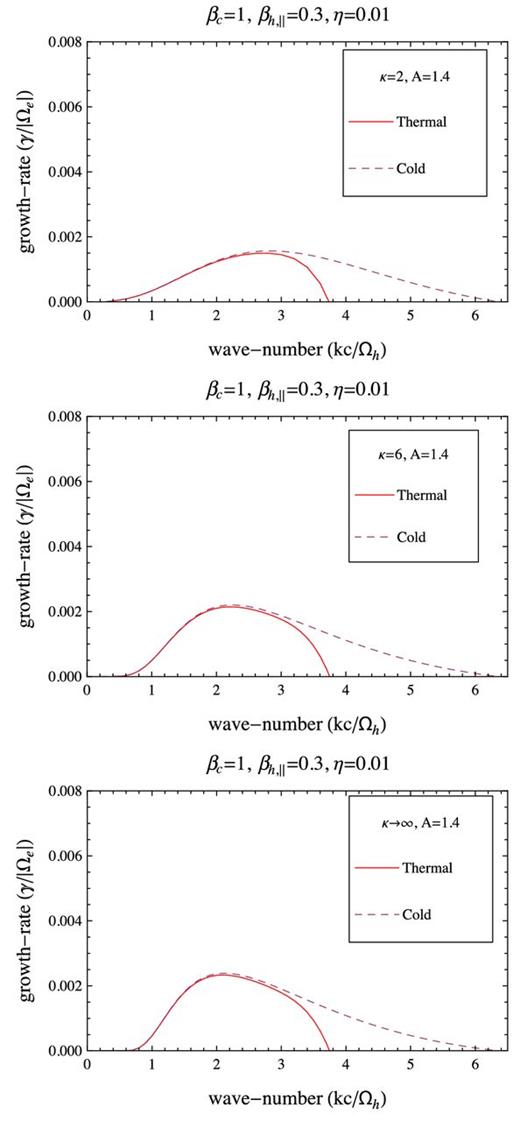
Growth rates of the whistler instability as provided by our models with a thermal core with βc = 1 (solid red lines), and a cold core (dashed lines). Comparison is extended for three halo models with the same η = 0.01, βh, ∥ = 0.3 and A = 1.4, but different κ = 2 (top), κ = 6 (middle) and κ → ∞ (bottom).

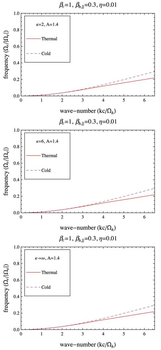
Frequency of the unstable modes in Fig. 10.
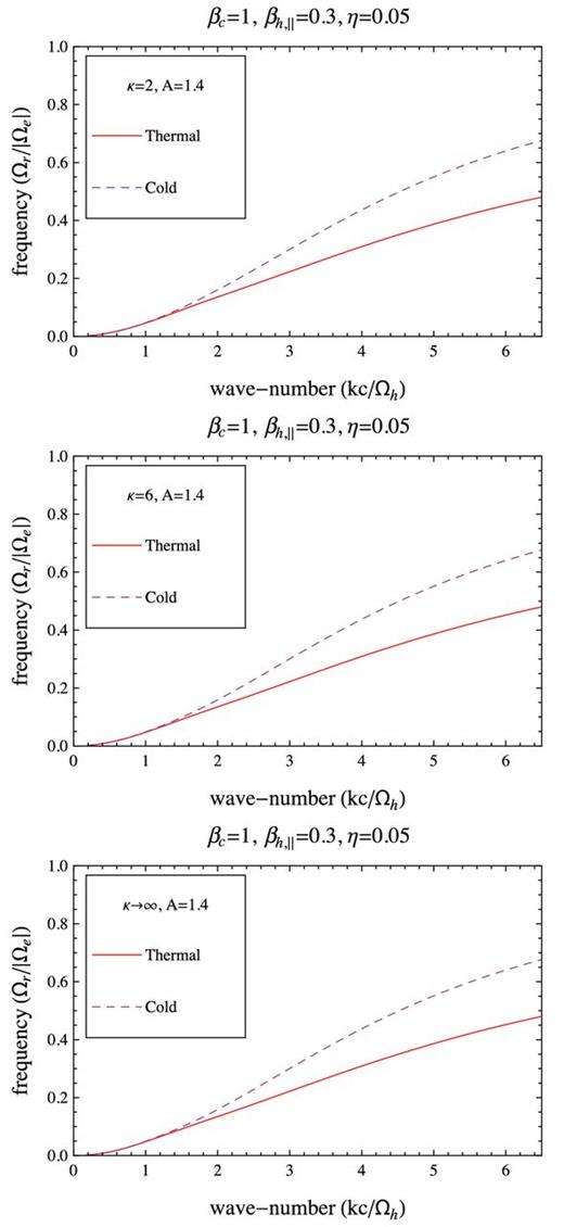
Frequency of the unstable modes in Fig. 11.
4 DISCUSSIONS AND CONCLUSIONS
In the analysis of space plasma instabilities, theoretical models currently invoked for the particle VDFs, see (a)–(d) in the Introduction, are too simplified to fully explain the observations. These models are more convenient computationally, due to a reduced number of parameters, but in general omit important kinetic effects of plasma particles. For instance, the real instability conditions cannot be evaluated if we ignore the halo populations that obviously are anisotropic and enhance the instability, neither if we neglect the thermal spread in the core, which is hot enough (Tc > 104 K) in the solar wind, and dominates (with a number density exceeding 90 per cent of total density) the other components in the distribution. In the fast wind, the energetic strahl drifting along the magnetic field is another source of free energy. A general model to describe the anisotropic VDFs indicated by the observations and the resulting instabilities must include all plasma species (electrons and ions) and all their components: a bi-Maxwellian for the core, a bi-Kappa for the halo and another drifting Kappa (or Maxwellian) for the strahl. However, if all these components are present and anisotropic, the number of parameters increases considerably, and the dispersion/stability analysis becomes very complicated even in numerical computations.
Starting from these premises, in this work, we have identified reliable conditions in the solar wind under which such a general, realistic model may be simplified and made tractable in computations, see equation (8). These conditions are typically encountered in the slow wind, when the strahl is absent or markedly less pronounced than the fast wind, the core is nearly isotropic, and the main trigger of local instabilities is the anisotropic halo. This approach is more realistic than any other idealized model used before in theoretical predictions since it incorporates the main features of the VDFs observed in a large variety of space plasmas, namely a core of finite thermal spread and a Kappa-distributed halo. The two-population (core–halo) model may be sufficient to describe the VDFs in the solar wind at large distances from the Sun since the strahl population appears to be continuously diminished in the favour of the halo population that increases with heliocentric distance (Maksimovic et al. 2005).
In Section 3, we have applied this model to an analysis of the EMEC modes, which are driven unstable by an excess of electron temperature in the direction perpendicular to the magnetic field (T⊥ > T∥). These modes are associated with the wave turbulence observed in the dissipation range in space plasmas. Whether these plasma modes are locally generated or only transmitted through the solar wind, here we have shown that their properties are highly dependent on the shape of the VDF. Comparative analysis with the simplified models of VDFs, e.g. cold-core, or two Maxwellians, enabled us to unveil the effects of the hot core and the suprathermals. The magnetic field and plasma parameters used to build the models and the dispersion formalism are based on the Ulysses observational data and reports by Maksimovic et al. (2005) and Stverak et al. (2008, 2009).
The instability thresholds are found to be highly dependent on the key parameters of our models, viz. the halo plasma beta, the halo–core relative density (η) and the power-index κ. These dependences are less important for the idealized models making comparison easier. The first conclusion to be drawn is that instability thresholds are increased by the thermal spread of the electron core. Thresholds are shifted to higher values, especially in the low halo-beta regimes (βh, ∥ ≤ 0.1), when the halo populations driving the instability are less energetic. This effect is observed enhancing and extending to higher values of the plasma beta (βh, ∥ ∼ 0.5) if the halo is more populated by increasing the relative density η or the suprathermal component (at low κ → 2). In these regimes (i.e. high η but low βh), an enhance of the instability due to the increase of suprathermal populations is evident, but only for a realistic model with thermal core (in a cold-core approach the effect is opposite).
A supplementary analysis of the unstable solutions confirms the inhibiting effect of the thermal core by lowering the growth rates and frequencies. Moreover, the intervals of unstable wavenumbers are markedly reduced, limiting the occurrence of instability to low wavenumbers. The inhibiting effect is indeed enhanced by increasing η, and correlating with the recent observations on the increase of this parameter with heliocentric distance enables us to conclude that local conditions for exciting the EMEC instability at large radial distances in the solar wind are less favorable than predicted before.
Figs 6, 10 and 11 indicate that growth rates of the EMEC instability are in general diminished by enhancing suprathermal population (decreasing κ → 2). However, in Fig. 7, the instability growth rates provided by the thermal-core model for low halo betas and sufficiently high η are found to be enhanced by the suprathermals. This dual influence of the suprathermals on the EMEC modes is not new since it was also found for global Kappa models (Lazar et al. 2011, 2013). Comparing to a cold-core model, a single global Kappa incorporates both the core and halo populations and is probably more realistic because the core temperature is not neglected. On the other hand, to have both the core and halo populations described by the same parameters (e.g. density and temperature) as in a global Kappa, is convenient computationally, but in general is not confirmed by the observations. We can therefore conclude that suprathermal effects can be quantified correctly only taking into account the finite thermal spread of the core. Moreover, the interplay of the core and halo populations appears to be decisive in the mechanism of instability, and future studies should clarify this aspect.
The authors acknowledge use of the Ulysses/SWOOPS electron data from the ESA-RSSD Web service ftp://www.rssd.esa.int/pub/ulysses/data/swoops/, and Ulysses 1-h averaged measurements of magnetic field and solar wind bulk speed data ftp://spdf.gsfc.nasa.gov/pub/data/ulysses/merged/. The authors acknowledge support from the Katholieke Universiteit Leuven, Grant no. SF/12/003, and from the Ruhr-Universität Bochum, the Deutsche Forschungsgemeinschaft (DFG), Grant Schl 201/25-1. These results were obtained in the framework of the projects GOA/2015-014 (KU Leuven), G.0729.11 (FWO-Vlaanderen) and C 90347 (ESA Prodex 9). The research leading to these results has also received funding from the European Commission's Seventh Framework Programme (FP7/2007-2013) under the grant agreements SOLSPANET (project n 269299, www.solspanet.eu) and eHeroes (project n 284461, www.eheroes.eu).
For the cold-core model, the inhibiting effect of the suprathermals has been shown first time by Xiao et al. (2006). The same effect was found for a global bi-Kappa model, but only for sufficiently large anisotropy, i.e. A ≥ 2 (Lazar et al. 2011), otherwise, at lower anisotropy 1 < A < 2, the effect is opposite (instability is enhanced by suprathermals), see Mace (1998) and Mace & Sydora (2010).
REFERENCES
APPENDIX A: FITTING PARAMETERS FOR THE ANISOTROPY THRESHOLDS
Here, we present four Tables A1 –A4 with values of the fitting parameters in equation (19), as derived for the unstable solutions of the thermal-core (T) model, equation (16), and the cold-core (C) model, equation (17)
Fitting parameters for thresholds in Fig. 2: |$\eta = n_{\rm h}/n_{\rm c} = \omega _{{\rm e},{\rm h}}^2 / \omega _{{\rm e},{\rm c}}^2 = 0.05$|, ωi/|Ωe| = 10−2.
| κ = 2 | κ = 6 | κ → ∞ | ||||
|---|---|---|---|---|---|---|
| Fit | T | C | T | C | T | C |
| a | 0.54 | 0.26 | 0.43 | 0.19 | 0.40 | 0.17 |
| b | 0.21 | −0.01 | 0.17 | −0.09 | 0.10 | −0.11 |
| c | 0.14 | 1.18 | 0.02 | 1.11 | 0.05 | 1.18 |
| d | 1.28 | 0.56 | 2.04 | 0.63 | 1.26 | 0.65 |
| κ = 2 | κ = 6 | κ → ∞ | ||||
|---|---|---|---|---|---|---|
| Fit | T | C | T | C | T | C |
| a | 0.54 | 0.26 | 0.43 | 0.19 | 0.40 | 0.17 |
| b | 0.21 | −0.01 | 0.17 | −0.09 | 0.10 | −0.11 |
| c | 0.14 | 1.18 | 0.02 | 1.11 | 0.05 | 1.18 |
| d | 1.28 | 0.56 | 2.04 | 0.63 | 1.26 | 0.65 |
Fitting parameters for thresholds in Fig. 3: |$\eta = n_{\rm h}/n_{\rm c} = \omega _{{\rm e},{\rm h}}^2 / \omega _{{\rm e},{\rm c}}^2 = 0.05$|, ωi/|Ωe| = 10−3.
| κ = 2 | κ = 6 | κ → ∞ | ||||
|---|---|---|---|---|---|---|
| Fit | T | C | T | C | T | C |
| a | 0.10 | 0.01 | 0.08 | 0.005 | 0.07 | 0.003 |
| b | 0.30 | −0.46 | 0.38 | −0.52 | 0.31 | −0.67 |
| c | 0.09 | 19.1 | 0.003 | 14.6 | 0.02 | 21.3 |
| d | 1.22 | 0.97 | 2.54 | 1.07 | 1.23 | 1.23 |
| κ = 2 | κ = 6 | κ → ∞ | ||||
|---|---|---|---|---|---|---|
| Fit | T | C | T | C | T | C |
| a | 0.10 | 0.01 | 0.08 | 0.005 | 0.07 | 0.003 |
| b | 0.30 | −0.46 | 0.38 | −0.52 | 0.31 | −0.67 |
| c | 0.09 | 19.1 | 0.003 | 14.6 | 0.02 | 21.3 |
| d | 1.22 | 0.97 | 2.54 | 1.07 | 1.23 | 1.23 |
Fitting parameters for thresholds in Fig. 4: |$\eta = n_{\rm h}/n_{\rm c} = \omega _{{\rm e},{\rm h}}^2 / \omega _{{\rm e},{\rm c}}^2 = 0.01$|, ωi/|Ωe| = 10−2.
| κ = 2 | κ = 6 | κ → ∞ | ||||
|---|---|---|---|---|---|---|
| Fit | T | C | T | C | T | C |
| a | 1.74 | 1.35 | 1.54 | 1.27 | 1.47 | 1.23 |
| b | 0.05 | −0.04 | 0.06 | −0.03 | 0.05 | −0.03 |
| c | 0.04 | 0.30 | 0.003 | 0.16 | 0.002 | 0.14 |
| d | 1.29 | 0.60 | 1.86 | 0.62 | 2.03 | 0.63 |
| κ = 2 | κ = 6 | κ → ∞ | ||||
|---|---|---|---|---|---|---|
| Fit | T | C | T | C | T | C |
| a | 1.74 | 1.35 | 1.54 | 1.27 | 1.47 | 1.23 |
| b | 0.05 | −0.04 | 0.06 | −0.03 | 0.05 | −0.03 |
| c | 0.04 | 0.30 | 0.003 | 0.16 | 0.002 | 0.14 |
| d | 1.29 | 0.60 | 1.86 | 0.62 | 2.03 | 0.63 |
Fitting parameters for thresholds in Fig. 5: |$\eta = n_{\rm h}/n_{\rm c} = \omega _{{\rm e},{\rm h}}^2 / \omega _{{\rm e},{\rm c}}^2 = 0.01$|, ωi/|Ωe| = 10−3.
| κ = 2 | κ = 6 | κ → ∞ | ||||
|---|---|---|---|---|---|---|
| Fit | T | C | T | C | T | C |
| a | 0.21 | 0.11 | 0.18 | 0.11 | 0.17 | 0.11 |
| b | 0.12 | −0.07 | 0.14 | −0.06 | 0.15 | −0.05 |
| c | 0.04 | 0.84 | 0.001 | 0.47 | 0.0001 | 0.40 |
| d | 1.28 | 0.60 | 2.21 | 0.63 | 2.83 | 0.64 |
| κ = 2 | κ = 6 | κ → ∞ | ||||
|---|---|---|---|---|---|---|
| Fit | T | C | T | C | T | C |
| a | 0.21 | 0.11 | 0.18 | 0.11 | 0.17 | 0.11 |
| b | 0.12 | −0.07 | 0.14 | −0.06 | 0.15 | −0.05 |
| c | 0.04 | 0.84 | 0.001 | 0.47 | 0.0001 | 0.40 |
| d | 1.28 | 0.60 | 2.21 | 0.63 | 2.83 | 0.64 |
