


Abstract
Dwarf spheroidal (dSph) galaxies are among the most promising targets for the indirect detection of dark matter (DM) from annihilation and/or decay products. Empirical estimates of their DM content – and hence the magnitudes of expected signals – rely on inferences from stellar-kinematic data. However, various kinematic analyses can give different results and it is not obvious which are most reliable. Using extensive sets of mock data of various sizes (mimicking ‘ultrafaint’ and ‘classical’ dSphs) and a Markov Chain Monte Carlo engine, here we investigate biases, uncertainties and limitations of analyses based on parametric solutions to the spherical Jeans equation. For a variety of functional forms for the tracer and DM density profiles, as well as the orbital anisotropy profile, we examine reliability of estimates for the astrophysical J- and D-factors for annihilation and decay, respectively. For large (N ≳ 1000) stellar-kinematic samples, typical of ‘classical’ dSphs, errors tend to be dominated by systematics, which can be reduced through the use of sufficiently general and flexible functional forms. For small (N ≲ 100) samples typical of ‘ultrafaints’, statistical uncertainties tend to dominate systematic errors and flexible models are less necessary. We define an optimal strategy that would mitigate sensitivity to priors and other aspects of analyses based on the spherical Jeans equation. We also find that the assumption of spherical symmetry can bias estimates of J (with the 95 per cent credibility intervals not encompassing the true J-factor) when the object is mildly triaxial (axis ratios b/a = 0.8, c/a = 0.6). A concluding table summarizes the typical error budget and biases for the different sample sizes considered.
1 INTRODUCTION
γ-ray observations of dark matter (DM)-rich systems have proven a competitive and complementary path to other DM indirect detection approaches. Exotic γ-ray signals have been looked for at the Galactic Centre (Abramowski et al. 2011; Hooper & Goodenough 2011; Weniger 2012; Daylan et al. 2014), in clusters of galaxies (Ackermann & Fermi LAT Collaboration 2010; Arlen et al. 2012), in Galactic dark clumps (Nieto et al. 2011; Ackermann & Fermi LAT Collaboration 2012) and in dwarf spheroidal (dSph) galaxies orbiting the Milky Way (Ackermann & Fermi-LAT Collaboration 2011; Geringer-Sameth & Koushiappas 2011; Ackermann & Fermi-LAT Collaboration 2014). The latter are interesting targets because of their proximity, potentially high DM densities and small astrophysical γ-ray backgrounds (Lake 1990; Evans, Ferrer & Sarkar 2004). As a result, dSphs can provide a crucial check on DM interpretations of γ-ray signals from high-background environments such as the Galactic Centre.
Recent Fermi-LAT results (Ackermann & Fermi-LAT Collaboration 2011, 2014; Geringer-Sameth & Koushiappas 2011) show that indirect detection in dSph galaxies can play a significant role in constraining the nature of DM. Given the instrument sensitivity and lack of an obvious signal, limits on 〈σv〉 are now reaching the canonical 3 × 10⁻²⁶ cm3 s−1 below which most supersymmetric DM models lie (Feng 2010). It therefore becomes critical to review how the most common underlying assumptions made in deriving these limits may affect or bias the results. Rather than on particle physics aspects, this paper will focus solely on the astrophysical assumptions (e.g. DM profile parametrization, velocity anisotropy and light-profile modelling) needed to compute astrophysical J- and D-factors (and their uncertainties). The D-factor allows constraints on the lifetime τ of decaying DM (Essig, Sehgal & Strigari 2009; Palomares-Ruiz & Siegal-Gaskins 2010), while the J-factor is required in computing limits on 〈σv〉 for annihilating DM. The body of this paper focuses mainly on the latter, while the corresponding results for the D-factor are similar and discussed in appendices.
To estimate the J- and D-factors, different authors rely on different priors in order to recover the mass and density profiles of the dSph galaxies. In many studies, DM density profiles are fitted directly to the kinematic data of the dSph under scrutiny (Bergström & Hooper 2006; Sánchez-Conde et al. 2007; Bringmann, Doro & Fornasa 2009; Pieri, Lattanzi & Silk 2009; Pieri et al. 2009), while others use ‘cosmological priors’ from structure formation simulations (Strigari et al. 2007; Martinez et al. 2009). These priors are uncertain in the absence of a complete understanding of the role of baryons, and can bias the results for systems in which little kinematic information is available, such as for ultrafaint dSph galaxies. The latter, such as Segue I, Willman I or Coma Berenices, are playing an increasing role in setting limits from γ-ray indirect searches, their short distances (∼20–40 kpc) allowing for higher values of J and therefore more stringent constraints on 〈σv〉. Only a few studies do not use strong priors for the DM profiles (Essig et al. 2009; Charbonnier et al. 2011; Walker et al. 2011), allowing for a data-driven analysis which provides larger, hence more conservative, error bars.
In this paper, we focus on data-driven analyses that rely on parametric solutions to the spherical Jeans equation (e.g. Strigari et al. 2006; Walker et al. 2010; Charbonnier et al. 2011). While Charbonnier et al. (2011) have previously examined some limitations inherent to this approach regarding the analysis of relatively luminous, ‘classical’ dSphs, here we use simulated data sets of various sizes in order to compare the relative importance of systematic errors for analyses of classical and ‘ultrafaint’ dSphs. In each case, we identify which modelling assumptions are most critical in terms of J- and D-factor determination, and suggest safer options whenever possible. In a forthcoming paper, we will apply the findings of this analysis to real data in order to provide robust J- and D-factor values for classical and ultrafaint dSph galaxies.
This paper is organized as follows. In Section 2, we cover all the ingredients needed in this study, namely the spherical Jeans equation, the computation of astrophysical J- and D-factors, the Markov Chain Monte Carlo (MCMC) algorithm and the description of the simulated data used. In Section 3, we highlight differences of our analysis with respect to that of Charbonnier et al. (2011). In Section 4, we run the Jeans analysis in the ideal case where the light and velocity anisotropy profiles are known, allowing us to study the impact of the DM density profile parametrization and evaluate the minimal uncertainties related to the sample size. The impact of the modelling of the velocity anisotropy and the light profile are then discussed in Sections 5 and 6, as well as the biases introduced when assuming spherical symmetry for triaxial DM haloes (Section 7). Finally, we discuss our results and conclude in Section 8.
2 JEANS ANALYSIS, J-FACTORS, MCMC AND MOCK DATA
2.1 Jeans analysis of dSph kinematics
Estimation of DM indirect detection signals from dSph galaxies requires knowledge of their mass density profiles, which have been particularly investigated in the last decade, thanks to the increase of kinematic measurements. Different techniques (Jeans models, Schwarzschild models, distribution function models, made-to-measure models, etc.) have been developed to infer the mass profile from stellar kinematic data and we refer the reader to recent reviews (and references therein) by Walker (2013), Battaglia, Helmi & Breddels (2013), Strigari (2013) for comprehensive descriptions of these methods. Here, we focus solely on analyses that use parametric functions for velocity anisotropy, tracer and DM density profiles in order to solve the spherically symmetric Jeans equation, which has been widely applied to dSph stellar kinematics (Strigari et al. 2007; Essig et al. 2010; Charbonnier et al. 2011; Walker et al. 2011).
2.1.1 Dark matter profiles
We use two families of DM profiles in this study:
- Zhao profiles (Hernquist 1990; Zhao 1996). This family of profiles requires three slope parameters (α, β, γ), the values of which allow the recovery of several DM profiles used in the literature (e.g. core, NFW, Moore). It is parametrized aswith ρs the normalization, rs the scale radius, γ the inner slope, β the outer slope and α the transition slope. Note that with this definition, ρs = ρ(rs) × 2(β − γ)/α.(8)\begin{equation} \rho _{\rm DM}^{\rm Zhao}(r)=\frac{\rho _s}{(r/r_s)^\gamma \times [1+(r/r_s)^\alpha ]^{(\beta -\gamma )/\alpha }} \end{equation}
- Einasto profiles (e.g. Merritt et al. 2006). This second family of profiles, using a logarithmic inner slope, was found to better fit DM haloes in numerical simulations (Navarro et al. 2004; Springel et al. 2008):where r−2 is the radius for which the logarithmic slope equals −2, and α controls the logarithmic slope sharpness.(9)\begin{equation} \rho _{\rm DM}^{\rm Einasto}(r)=\rho _{-2} \exp \left\lbrace -\frac{2}{\alpha }\left[\left(\frac{r}{r_{-2}}\right)^\alpha -1\right]\right\rbrace , \end{equation}
2.1.2 Light profiles
Stellar surface brightnesses of dSphs are generally fitted using Plummer (1911), King (1962) or Sersic (1968) profiles (e.g. Irwin & Hatzidimitriou 1995), but exponential and Zhao (for the 3D stellar density) profiles have also been considered. De-projection (or projection in the Zhao case) of these profiles rely on the Abel transform of equation (5), which may be analytically computed in some cases. We give below the adopted parametrizations and refer the reader to the associated references for de-projected analytical formulae (for the Plummer, exponential and King cases).
- The Plummer profile (Plummer 1911) readswith L the total luminosity, and rhalf the projected half-light radius.(10)\begin{equation} I^{\rm Plummer}(R)=\frac{L}{\pi r_{\rm half}^2}\frac{1}{[1+R^2/r_{\rm half}^2]^2}, \end{equation}
- The exponential profile (Evans, An & Walker 2009) is parametrized aswith I0 the normalization, and rc the scale radius of exponential decrease.(11)\begin{equation} I^{\rm exp}(R)=I_0 \times \ \exp \left(-\frac{R}{r_c}\right)\,, \end{equation}
- The King profile (King 1962) is written aswith I0 the normalization, rc the ‘core’ radius and rlim the maximum radius beyond which the density goes to zero.(12)\begin{equation} I^{\rm King}(R)=I_0 \times \left[\left(1+\frac{R^2}{r_c^2}\right)^{-1/2} -\left(1+\frac{r_{\rm lim}^2}{r_c^2}\right)^{-1/2}\right], \end{equation}
- The Sérsic profile (Sersic 1968; Prugniel & Simien 1997) readswith bn = 2n − 1/3 + 0.009876/n, I0 the normalization, n ≳ 0.5 an irrational number (controlling the sharpness of the logarithmic decrease) and rc a scale radius.(13)\begin{equation} I^{\rm S\acute{e}rsic}(R)=I_0 \times \ \exp \left\lbrace -b_n \times \left[ \left(\frac{R}{r_c}\right)^{1/n} - 1 \right]\right\rbrace , \end{equation}
- Finally, the Zhao profile (Hernquist 1990; Zhao 1996) given by equation (8) is here applied to the 3D (i.e. unprojected) light profile,In this case, the light profile is analytical for the 3D density profile ν(r) but has to be numerically projected along the l.o.s. to provide the surface brightness I(r).(14)\begin{equation} \nu ^{\rm Zhao}(r)=\rho _{\rm DM}^{\rm Zhao}(r). \end{equation}
As already mentioned, we assume that DM dominates the gravitational potential at all radii (all measured dSphs have central mass-to-light ratios ≳ 10, e.g. Mateo 1998), so that the value of the normalization factor (L or I0) has no bearing on the analysis.
2.1.3 Velocity anisotropy profiles
- The constant anisotropy modelling (e.g. used by Charbonnier et al. 2011) simply reads(16)\begin{equation} \beta _{\rm ani}^{\rm Cst}(r)=\beta _0. \end{equation}
- The Osipkov–Merritt profile (Osipkov 1979; Merritt 1985) is parametrized aswith a single free scale parameter ra which locates the transition from βani = 0 in the inner parts (isotropic) to 1 at large radii (full radial anisotropy).(17)\begin{equation} \beta _{\rm ani}^{\rm Osipkov}(r)=\frac{r^2}{r^2+r_a^2}, \end{equation}
- The Baes and van Hese profile (Baes & van Hese 2007) is more general and is written aswhere the four parameters are the central anisotropy β0, the anisotropy at large radii β∞, and the sharpness of the transition η at the scale radius ra. The Osipkov–Merritt profile is recovered when using β0 = 0, β∞ = 1 and η = 2.(18)\begin{equation} \beta _{\rm ani}^{\rm Baes}(r) =\frac{\beta _0 + \beta _\infty (r/r_a)^\eta }{1+(r/r_a)^\eta }\,, \end{equation}
2.1.4 Technicalities (for the Jeans solution)
As seen from equations (3), (4) and (6), the solution of the projected Jeans equation requires in principle three successive integrations. However, as shown by Mamon & Łokas (2005, 2006), the calculation of equation (6) for constant and Osipkov–Merritt anisotropy profiles (and many others) can be cast as a single integration. This tremendously speeds up the calculation with respect to the Baes & van Hese profile case, for which no shortcut was found in the literature.
All the Jeans analyses presented here are performed with a new module of the clumpy2 code (Charbonnier, Combet & Maurin 2012), which was developed and used to calculate J- and D-factors (Charbonnier et al. 2011; Walker et al. 2011; Combet et al. 2012; Maurin et al. 2012; Nezri et al. 2012). The new Jeans analysis module was validated by systematic cross-checks with the results (obtained with a different code and MCMC engine) of Charbonnier et al. (2011); it will be made publicly available in the second release of clumpy (Bonnivard et al., in preparation).
2.2 Astrophysical factor for annihilation and decay
The J-factor (resp. D-factor) is useful knowledge as it allows us to rank the DM targets (in terms of their expected γ-ray flux) independently of the details and couplings of the underlying particle physics model.
For annihilating DM, the well-established presence of substructures in DM haloes (e.g. Springel et al. 2008) can boost the signal. However, the smaller the host halo mass, the less boosted the signal is (e.g. Sánchez-Conde & Prada 2014). Taking generic configurations of the substructure distribution and the host halo parameters, Charbonnier et al. (2011) found that DM substructures in dSph galaxies do not significantly boost the annihilation signal. In a completely different approach and in the context of the Milky Way DM halo, the role of fine-grained phase-space structures (haloes and streams) was studied in details in Vogelsberger & White (2011), who found a very small impact on the annihilation signal and also on the variance of the mean density. These results motivate the description of the total DM halo of dSph galaxies as a smooth density, whose reconstructed profile (by means of the Jeans analysis) can be interpreted as the sum of the smooth halo plus the mean density of substructures.
2.3 Likelihood, MCMC, posteriors and credibility intervals
For a given choice of DM density and velocity anisotropy parameters, we compare the projected velocity-dispersion profile σp(R) calculated from equation (6) to the observed one σobs(R). The latter is reconstructed from individual stellar velocities (see next section), while the projected light profile I(R) – used to compute the velocity dispersion – is fitted separately (see Section 6).
Markov chain Monte Carlo (MCMC). In order to efficiently explore the large parameter space (up to nine free parameters for a Zhao DM profile and a Baes & van Hese anisotropy profile), we employ an MCMC technique (Neal 1993). Based on Bayesian parameter inference, this method allows for an efficient sampling of the posterior probability density function (PDF) of a vector of parameters |$\boldsymbol{\theta }$| using Markov chains. From the PDFs, credibility intervals (CIs) for any quantity of interest are easily computed. In this analysis, we use the Grenoble Analysis Toolkit (GreAT): it is a modular c++ framework dedicated to statistical data analysis (Putze 2011, Putze & Derome 2014), originally developed for cosmic ray physics studies (Putze et al. 2009; Putze, Derome & Maurin 2010; Putze, Maurin & Donato 2011). It relies on the Metropolis–Hastings algorithm to sample the posterior distributions (Metropolis et al. 1953; Hastings 1970). The number of chains used (with typically 25 000 points/chain) depends on the number of free parameters and on the size of the mock sample (see next section); it typically varies from a few to more than 100 chains, in order to gather a sufficient number of points to calculate CIs. The proposal function used in this work is a multivariate Gaussian distribution. We provide in Appendix A specific combinations of the DM parameters to improve the efficiency of the MCMC in the context of the Jeans analysis.
Posterior distributions. The posterior distributions are obtained after several post-processing steps (burn-in length removal, correlation length estimation and thinning of the chains) required to ensure the insensitivity of the result to the initial conditions and independent sample selection. Note that in a Bayesian analysis, the priors used for each parameter can strongly impact the results, especially if the parameters are loosely constrained. We restrict this study to uniform priors, and the extensive use of mock data allows us to define ‘optimal’ ranges, for instance for DM profile parameters (see Table 1), as further discussed in Sections 4 and 5.
Range of uniform priors used for the DM profile parameters. Adding the conditions reported in the last column leads to better (more constrained) credibility intervals.
| DM profile | Parameter | Prior | Added condition | |
|---|---|---|---|---|
| ‘Zhao’ | log10(ρs/M⊙kpc−3) | [5, 13] | – | |
| equation (8) | log10(rs/kpc) | [ − 3, 1] | |$r_{s} \ge r_{s}^{*}$| | (Section 4.1) |
| α | [0.5, 3] | – | ||
| β | [3, 7] | – | ||
| γ | [0, 1.5] | γ ≤ 1 | (Section 5) | |
| ‘Einasto’ | log10(ρ−2/M⊙kpc−3) | [5, 13] | – | |
| equation (9) | log10(r−2/kpc) | [−3, 1] | |$r_{-2} \ge r_{s}^{*}$| | (Section 4.1) |
| α | [0.05, 1] | α ≥ 0.12 | (Section 5) | |
Criterion to select the best analysis setup. We remind that the ultimate goal of the analysis is to determine the best setup (or best estimator) to calculate the J-factors of Milky Way's dSph galaxies. This selection is made on mock data (see next section). The different estimators used are associated with different assumptions made for the input parameters (DM profile, light and anisotropy profile, see previous section). A statistically sound approach would be to characterize each estimator (bias, mean square error, consistency, etc.), by running many realizations of the data for each setup. This is however too computationally demanding. The approach followed here is to use a restricted (but still sizeable) set of samples to study several setups and the performances of the associated estimators (namely the binned likelihood from equation (20) for different models/configurations). Following Charbonnier et al. (2011), we use the median values as the estimator of the true value (see their Appendix F). The relative merit of the different setups tested is assessed by comparing the distribution of distances of the median and CIs to the true value of the mock data at hand. In particular, any trend for a systematic offset of the median distribution to the true values will be denoted ‘bias’ (which is a small misuse of the word in the statistical context). A particular setup for an analysis will be said to be strongly biased if the reconstructed quantities do not encompass the true value at the 95 per cent level. In the following, we choose the best estimator to be the least biased (if possible) and the one leading to the smallest CIs.
2.4 Mock data
In order to examine the performance of analyses that employ various assumptions, we analyse three suites of mock data sets that consist of stellar positions and velocities drawn from static distribution functions that satisfy the collisionless Boltzmann equation. The first suite is the same one used previously by Walker et al. (2011) and Charbonnier et al. (2011). Briefly, it randomly samples distribution functions of the form |$L^{-2\beta _{\rm ani}}f(\epsilon )$|, where ϵ is energy and L is angular momentum. For given choices of ρDM(r) and ν(r), the distribution functions are computed numerically using the method of Cuddeford (1991). All models in this suite have stellar components described by3 α★ = 2, β★ = 5, and DM haloes described by αDM = 2, βDM = 3.1, with normalization ρs chosen such that the mass enclosed within the central 300 pc is M300 ∼ 107 M⊙. Other than this normalization, the parameters that vary from model to model are then γDM, r★, rs, βani and γ★. We consider cases with γDM between 0 and 1, γ★ between 0 and 0.7, rs between 0.2 and 1 kpc, and r★/rs between 0.1 and 1, allowing for cored profiles, NFW-like cusps and a large range of stellar concentrations. For each potential, the anisotropy is constant, with values between βani = −0.45 (tangential anisotropy) and βani = +0.3 (radial). These combinations of parameters yield a suite of 64 unique models.
The second suite of mock data sets is similar to the one used by Walker & Peñarrubia (2011) and is available and described in detail as part of The Gaia Challenge, a community-wide effort to examine the performance of various methods on common test problems.4 Briefly, these samples are generated from the family of spherical, anisotropic distribution functions originally proposed by Osipkov (1979) and Merritt (1985). Thus, they have anisotropy profiles of the form given by equation (17). For given ρDM(r) and ν(r), the distribution functions are calculated using equation 11 of Merritt (1985) and then sampled using an accept–reject algorithm. All models in this suite have stellar components with α★ = 2, β★ = 5, and DM haloes with αDM = 1, βDM = 3 and rs = 1 kpc, again with normalization ρs chosen such that M300 ∼ 107 M⊙. Other parameters that vary from model to model are r★, γ★, γDM, and the anisotropy radius ra. We consider cases with γDM = 0, 1, γ★ = 0.1, 1, r★/rs = 0.1, 0.25, 0.5, 1 and ra = r★, ∞, allowing 32 unique models. Note that for ra = ∞, the anisotropy profile is equivalent to a constant profile with βani = 0. The third and final suite of mock data sets is also available and described in detail as part of The Gaia Challenge, but in this case the underlying models are triaxial and therefore violate the common assumption of spherical symmetry. These samples are generated using the ‘made-to-measure’ N-body code of Dehnen (2009). There are two unique models in this suite, and both have axis ratios (for both halo and tracer components) b/a = 0.8 and c/a = 0.6, with spherically averaged profiles described by equation (8), with αDM = 1, βDM = 4, rs = 1.5 kpc, α★ = 2.9, β★ = 5.92, γ★ = 0.23 and r★ = 0.81 kpc. Parameters that vary from one case to the other are γDM, which takes values of either 0.23 or 1.0, and ρDM, which takes values of 5.5 × 10⁷ M⊙ kpc−3 (for cases with γDM = 1) or 1.2 × 10⁸ M⊙ kpc−3 (for cases with γDM = 0.23).
Table 2 summarizes the three suites of synthetic data. For each model, we draw samples of N = 30 (small), 1000 (medium) and 10 000 (large) stars in order to encompass the range of stellar-kinematic data sets currently available for ultrafaint and classical dSphs, as well as for ‘ideally observed’ dSphs. For each sample, we estimate the ‘observed’ velocity-dispersion profile by projecting mock data along one of the principle axes, parsing the sample into |$\sqrt{N}$| bins that each contain |$\sqrt{N}$| mock observations (except for the ‘small’ samples of N = 30, for which we take two bins, each with 15 stars), and then computing the projected velocity dispersion (and its variance) using the maximum-likelihood technique as discussed by Walker et al. (2006). All our mock data are free of background and foreground contaminations, which represent additional, though independent, sources of systematic effects for the quantities reconstructed (DM profile, J- and D-factors). The star contaminations will be discussed in a separate study in the context of the analysis of real dSph data. Fig. 1 shows examples of velocity-dispersion profiles calculated for small, medium and large mock samples. For the calculation of the J- and D-factors, all the mock dSphs are assumed to correspond to objects at a fixed distance d = 100 kpc.
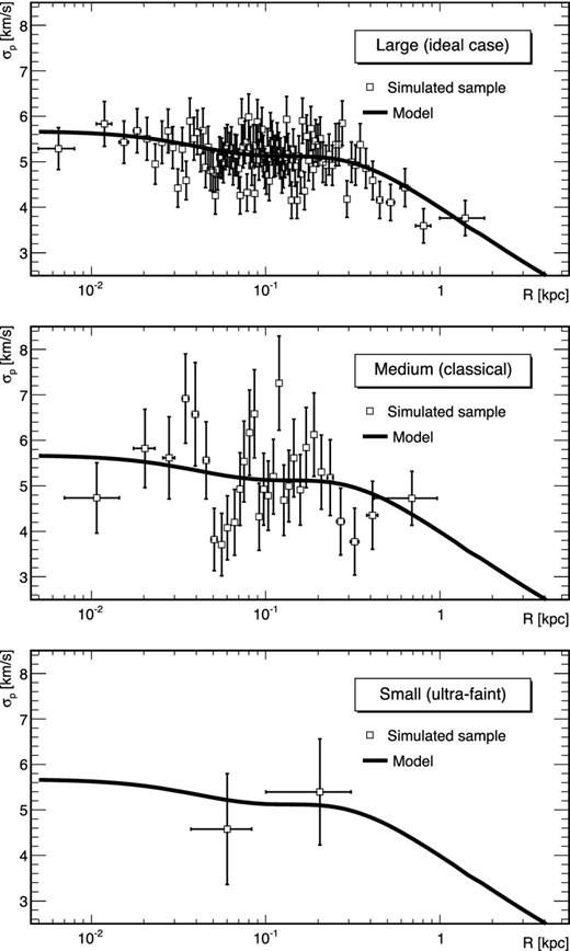
Velocity-dispersion profile obtained for three sample sizes of a same model. Top: large sample, with 10 000 stars (ideal case). Middle: medium sample, with 1000 stars, corresponding to a classical dSph. Bottom: small sample, with 30 stars, mimicking an ultrafaint dSph.
Properties of the three sets of simulated data used in this study. Two of them come from The Gaia Challenge (astrowiki.ph.surrey.ac.uk/dokuwiki). DM and light profiles are Zhao – equation 8. γ refers to the logarithmical inner slope of the DM and light profiles of the models, rs to their scale radii, and βani to their velocity anisotropy.
| Mock data | Sphericala | Sphericalb | Triaxialc |
|---|---|---|---|
| Number of models | 64 | 32 | 2 |
| γ | [0, 1] | 0 − 1 | 0.23 − 1 |
| rs (kpc) | [0.2, 1] | 1 | 1.5 |
| γ★ | [0, 0.7] | 0.1 − 1 | 0.23 |
| rs★ (kpc) | [0.1, 1] | [0.1, 1] | 0.81 |
| βani profile | Cst | Cst+Osipkov | Baes & van Hese |
3 PRELIMINARY DISCUSSION
Fig. 2 illustrates (for one of the models and small sample size) the main functions of interest in this study: the projected velocity-dispersion profile, σp(R) (top left), the DM density profile ρDM(r) (top right), and the J- and D-factors calculated (using equation 19) as functions of the integration angle αint (bottom panels). In each panel, and in almost all plots shown in this paper, the thick black lines are reference curves, calculated with the true (i.e. known) parameters, to which the MCMC results are compared.
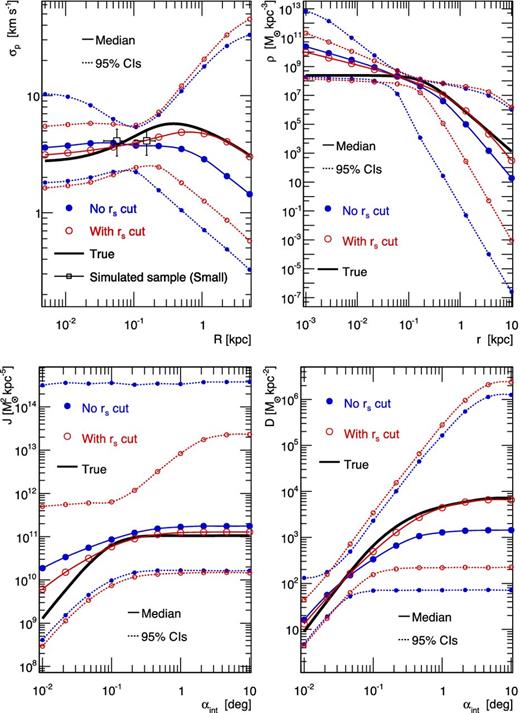
Median values (solid lines with symbols) and 95 per cent CIs (thin dashed lines with symbols) for the velocity-dispersion profile (top left), the DM density profile (top right), the J-factor (bottom left) and the D-factor (bottom right). Enforcing the condition |$r_s \ge r_s^\star$| (red empty circles compared to blue filled circles) in the prior of the MCMC analysis (see Table 1) leads to better results, i.e. with the median value closer to the true value with smaller uncertainties (less biased and better estimator). The model shown corresponds to a mock ultrafaint dSph galaxy with γ = 0, rs = 0.2kpc and |$r_{s}^{*} = 0.1 {\rm kpc}$|.
On the top left panel, the empty squares correspond to the velocity-dispersion data used in the Jeans/MCMC analysis (small sample in this case). The median (solid lines with symbols) and the 95 per cent lower and upper CIs (dotted lines) are computed from equation (21). The two sets of blue and red curves, discussed in Section 4.1, correspond to different priors, and we focus on the red curves only (filled circles) for this preliminary discussion.
Before moving to our new results, it is useful to underline the similarities and differences with the analysis performed on the same mock data considered by Walker et al. (2011) and Charbonnier et al. (2011). In these papers, only medium-size samples were used (to be representative of classical dSphs data), with surface brightness profiles fitted with Plummer profiles, and with anisotropy assumed to be constant. The more thorough analysis of this paper allows us to get more insight into the modelling uncertainties, while reinforcing and extending the conclusions drawn from the previous analyses (Charbonnier et al. 2011; Walker et al. 2011). We briefly summarize below what conclusions these previous studies reached and underline what this new analysis brings.
Determination of the DM inner slope: for mock classical dSph galaxies (N ∼ 1000 stars), the DM profile inner slope γ was found not to be constrained by the Jeans analysis (Charbonnier et al. 2011). This is even more true for mock ultrafaint dSphs (see, e.g. the top right panel in Fig. 2, where all slopes γ ∈ [0, 1] are allowed at the 95 per cent level). The difficulty to constrain this slope is generally attributed to the degeneracy of the DM parameters with the anisotropy parameter βani(r), and methods relying on higher order of the Jeans analysis have been proposed to circumvent this issue (Richardson & Fairbairn 2013, 2014; Richardson, Spolyar & Lehnert 2014). See also the mamposst approach in Mamon, Biviano & Boué (2013). We find in Section 4 that this difficulty remains even with a perfect knowledge of the light profile and anisotropy, for any sample size. This indicates that constraining the inner slope in the standard Jeans modelling is limited by degeneracies among the DM profile parameters themselves. These degeneracies appear because of the poor sampling of the inner parts of dSph galaxies which remain difficult to measure. A better approach to address this issue may be to use different population tracers (e.g. Amorisco & Evans 2011; Walker & Peñarrubia 2011; Agnello & Evans 2012).
Determination of J independently of the exact γ value: while γ cannot be determined, it does not, however, prevent constraining the J-factor (Charbonnier et al. 2011, and bottom left panel of Fig. 2, where the true J-factor is encompassed within the CIs). A similar behaviour is found for decaying DM (illustrated by the bottom right panel of Fig. 2).
Optimal integration angle: one major finding of Walker et al. (2011) and Charbonnier et al. (2011) is the existence of an optimal integration angle for which the uncertainty on the J-factor is minimal. This is illustrated by the pinch visible in the red curves (with empty circles) in the bottom left panel of Fig. 2. This pinch is observed for all the quantities displayed – σp(R), ρ(r), J(αint) and D(αint). For the velocity-dispersion profile, the pinch occurs where most of the data lie, which is near the tracer scale radius |$r_s^\star$| (0.1 kpc for the model displayed). Because this is also the radius where the mass-anisotropy degeneracy is minimized (Walker et al. 2009; Wolf et al. 2010), ρ(r) is also relatively well constrained at this radius. In terms of the J-factor, the tightest constraint occurs when the signal is integrated over an angle |$\alpha _c^J\approx 2r_s^\star /d$| (Walker et al. 2011). We recall that d is taken to be 100 kpc throughout the paper, so that it corresponds to |$\alpha _c^J\sim 0.1^\circ$| in the bottom left panel of Fig. 2. As discussed in Appendix B, we find that for DM decay, the critical angle |$\alpha _c^D$| is half the one for annihilation DM: |$\alpha _c^D\approx \alpha _c^J/2\approx r_s^\star /d$|. For the model shown in the bottom right panel, |$\alpha _c^D\sim 0{^{\circ}_{.}}05$|.
These results will not be further discussed in the paper, which from here on focuses on effects that were not systematically (or not at all) studied in Charbonnier et al. (2011).
4 IMPACT OF THE DM MODELLING: MAXIMUM KNOWLEDGE SETUP
In this section, we use the mock data described in Section 2.4, in the idealized case where the light and anisotropy profiles are known and fixed to their true values (i.e. that were used to generate the mock data). This configuration, dubbed maximum knowledge, allows us to investigate the direct impact of the DM profile parametrization (Zhao or Einasto) and of its priors. The uncertainties obtained on ρ(r), J(αint) and D(αint) in this ideal case also give a flavour, for different sample sizes, of the precision that the Jeans modelling could reach for analyses improving on the light and anisotropy-related parameters.
The following results are based on three different sample sizes (see Section 2.4 and Fig. 1) of 64 spherical models (first column of Table 2). For each MCMC analysis, the only free parameters are the DM profile ones.
4.1 An optimal cut for the DM scale radius: |$\boldsymbol{r_s\ge r_s^\star }$|
Fig. 2 shows the results of the Jeans analysis for a typical mock ultrafaint dSph galaxy, where blue curves (with filled circles) are obtained using the prior log10(rs/kpc) ∈ [ − 3, 1], while red curves (with empty circles) are obtained using the range [ − 1, 1] (see also Table 1). The value −1 comes from the condition |$r_s\ge r_s^\star$| (with |$r_s^\star =0.1$| kpc for the model shown), i.e. demanding the DM scale radius to be larger than the light scale radius. Even knowing the value of the light and velocity anisotropy parameters, very large uncertainties appear on all quantities displayed in Fig. 2 (especially the J-factor). However, they are significantly reduced using the above cut on rs values (blue versus red curves).
A more detailed view of this effect is provided in Fig. 3 using the same colour code for the two different priors: PDFs of ρs and rs and their correlation are shown for the same model as in Fig. 2 (see Charbonnier et al. 2011 for a thorough discussion of DM parameter correlations). These plots illustrate that too-small rs lead to very high values of the DM density in the inner parts (see top left panel), which will propagate to large J- factors. Although unrealistic, these models fit well the poorly constrained velocity-dispersion profile (top left panel of Fig. 2). Note that whether the cut on rs values is applied or not, the Jeans analysis is unable to recover the correct values of the DM parameters (because of the degeneracy between them), even in this maximum knowledge configuration.
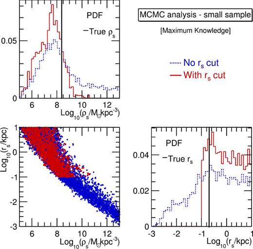
PDFs (diagonal) and correlation (off diagonal) of ρs and rs obtained from the maximum knowledge MCMC analysis (same mock dSph as in Fig. 2, and same colour code). With no cut on the rs prior (blue dashed line), the anticorrelation between the two gives rise to nonphysical models (with very low DM scale radii and very large densities). Applying the condition |$r_s\ge r_s^\star$| (equals to 0.1 kpc here), the two parameters are still poorly constrained (red solid lines), but nonphysical models are removed.
Following Charbonnier et al. (2011), we wish to rely on as ‘data-driven’ an approach as possible and therefore, do not want to adopt priors based on DM haloes produced in cosmological N-body simulations (cf. Martinez et al. 2009). The condition |$r_s\ge r_s^\star$| assumes that a DM halo must be at least as large as the stellar population it hosts, which seems inevitable so long as the stars form from gas that sinks to the centre of a DM halo as it cools (White & Rees 1978). This prior leads to less biased reconstructed values with smaller uncertainties for mock ultrafaint dSphs (see all panels in Fig. 2). The analysis has been repeated on the 64 mock dSph galaxies and for each, it always led to the same conclusion. Fig. 4 shows the distribution of |$J^{+95\,\mathrm{per\ cent}\ \rm CI}/J^{\rm true}$| values among the 64 models, before (blue dashed line) and after (red solid line) applying the condition |$r_s\ge r_s^\star$|. Before the cut, more than half of the models had |$10^2 J^{\rm true} \lesssim J^{+95\,\mathrm{per\ cent}\ \rm CI}\lesssim 10^6 J^{\rm true}$|. The improvement is significant once the cut is applied, with |$J^{+95\,\mathrm{per\ cent}\ \rm CI}\lesssim 100\,J^{\rm true}$| for all models (but one). This result is obtained for an integration angle αint = αc, but similar improvements are observed at other angles.5 This cut is less crucial for the mock classical samples (not shown), and has no effect for dSphs from the large sample. Note that the |$J^{-95\,\mathrm{per\ cent}\ \rm CI}$| values are not affected by this cut (bottom left panel of Fig. 2).
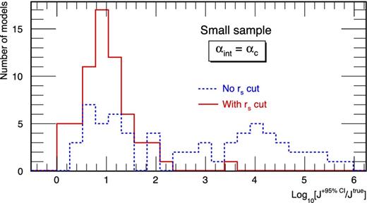
Distribution of |$J^{+95\,\mathrm{per\ cent}\ \rm CI}/J^{\rm true}$| for the 64 mock ultrafaint dSph galaxies, calculated at the critical angle |$\alpha _c= 2r_{s}^{*}/d$|. The condition |$r_s\ge r_s^\star$| (red solid line) produced smaller uncertainties compared to the case where no cut is applied (blue dashed line).
In the remainder of the paper, the cut on rs will always be applied. For the sake of legibility, only results related to the J-factors are discussed below: similar effects are generally observed for the other quantities (σp, ρ and D), and we refer the interested reader to Appendix D for results on D-factors.
4.2 Impact of the DM profile: Zhao versus Einasto
Jeans analyses of dSph galaxies have typically used NFW or core profiles (i.e. Zhao profiles with fixed slope parameters, e.g. Evans et al. 2004; Strigari et al. 2007), while Walker et al. (2011) and Charbonnier et al. (2011) have recently extended this approach to more generic Zhao haloes. Einasto profiles are also becoming a popular choice (e.g. Martinez et al. 2009; Essig et al. 2010). This section aims at checking if the choice of the DM profile parametrization has an impact on the J values. To do so, the results for the 64 models (and the three sample sizes) are compared, when processed using the five-parameter Zhao profile or the three-parameter Einasto profile.
The very good agreement (on a wide range of integration angles) between the two parametrizations is illustrated for one medium-size model (i.e. mock classical dSph) in Fig. 5, where J(αint) is plotted for both Zhao (blue filled circles) and Einasto (red empty circles) DM profiles. Median values and CIs are similar in both cases, with a small deviation occurring for very small integration angles, αint ≲ a few 10−2 deg. Fig. 6 compares the distribution of Jmedian/Jtrue values obtained using all the 64 models, at three integration angles (from top to bottom, 0.1αc, αc and 10αc). The distributions for the Zhao (dashed blue) and Einasto (solid red) cases are in very good agreement (the same conclusion holds for ρ and D calculations). There is an indication that the Einasto profile provides a slightly better fit for αint = 0.1αc (top panel) as the distribution appears more centred around zero. However, the effect is small and we only mention it as a possibility.
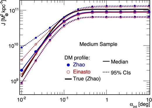
J-factor median values (solid lines with symbols) and 95 per cent CIs (thin dashed lines with symbols) for a mock classical dSph galaxy for which the light and anisotropy profiles are perfectly known. MCMC/Jeans analyses with a Zhao (blue filled circles) or an Einasto (red empty circles) DM profile give similar results, the latter being much faster to run (three free parameters instead of five). The true value (thick black solid line) is encompassed within the 95 per cent CIs.
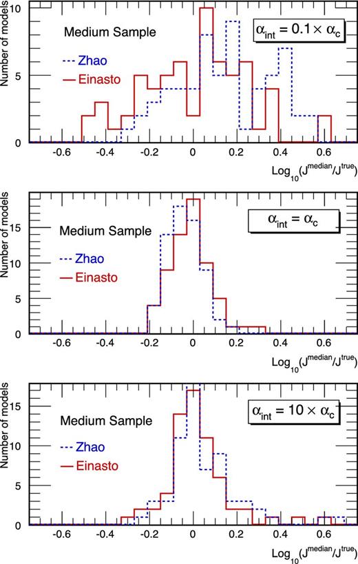
Distribution of Jmedian/Jtrue values for the 64 models in the medium-size configuration, for three integrations angles: 0.1αc (top), αc (middle) and 10αc (bottom). Using a Zhao (dashed blue lines) or an Einasto (red solid lines) parametrization gives similar results.
The Einasto DM profile has less free parameters than the Zhao parametrization, which allows for faster runs of the MCMC chains (fewer points required to reach convergence). Therefore, it is used in the remainder of the paper.
4.3 Importance of the sample size
Knowing the light and velocity anisotropy parameters, we can establish the best limits that could be reached (but not overcome) using the data-driven Jeans analysis (i.e. without strong cosmological priors), for classical and ultrafaint dSphs.
In Fig. 7, the left-hand column shows the distributions of the |$J^{+95\,\mathrm{per\ cent}\ \rm CI}/J^{\rm true}$| values of the 64 models in the maximum knowledge analysis: top to bottom panels correspond to different integration angles and the different colours/linestyles to the three sample sizes. As already underlined, the uncertainty on the J-factor is smaller for αint = αc (middle panel). At this optimal integration angle, the best limit expected to be set on the J-factor is uncertain up to a factor ∼3 for mock classical dSph galaxies (green dotted lines), and up to a factor ∼25 for mock ultrafaint ones (red dashed lines). For smaller (αint = 0.1αc, top panel) or larger (αint = 10αc, bottom panel) integration angles, these uncertainties are an order of magnitude larger. The |$J^{-95\,\mathrm{per\ cent}\ \rm CI}/J^{\rm true}$| distributions (not shown) have the same behaviour, with comparable widths.
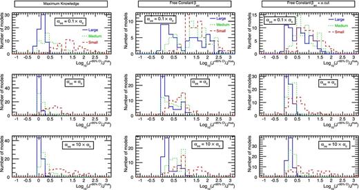
Distribution of |$J^{+95\,\mathrm{per\ cent}\ \rm CI}/J^{\rm true}$| values for the 64 dSph models. These plots show the impact of the data sample size – large sample in solid blue lines, mock classical dSph galaxies in dotted green lines, and mock ultrafaints in dashed red lines – on the J-factor uncertainties for ‘different’ Jeans analysis configurations (with Einasto DM profile priors set to Table 1 values and using |$r_{-2}\ge r_s^\star$|). Rows are different integration angles (0.1αc: top; αc: middle; 10αc: bottom), and columns are the different configurations. Left-hand panels: the setup is maximum knowledge (Section 4.3), i.e. known light and anisotropy parameters. Middle panels: as for the previous setup (free DM parameters), but with free constant anisotropy β0 (Section 5.2). Right-hand panels: as for the previous setup, but adding the cut α ≥ 0.12 on the Einasto slope (Section 5.2). See the text for a discussion of the plots. Note that the distributions are almost always positive, indicating that the reconstructed J-factors are not strongly biased with respect to the true values.
Note that smaller uncertainties are quoted in studies relying on analyses using ‘cosmological priors’ (e.g. Martinez 2013); however, our data-driven approach mitigates biases that would arise in the case that real dSphs are hosted by DM subhaloes that differ structurally from simulated ones. This would be the case if, for example, the DM differs from cold dark matter (CDM), as in ‘warm’ (Bode, Ostriker & Turok 2001) or ‘self-interacting’ (Spergel & Steinhardt 2000) DM models, or if feedback from star formation significantly alters the internal structure of low-mass subhaloes (Pontzen & Governato 2012) with respect to the CDM-only simulations from which otherwise-cosmological priors have been derived.
5 IMPACT OF THE ANISOTROPY PROFILE
The velocity anisotropy profile βani(r) needed in the Jeans modelling, equations (3) and (4), is degenerate with the mass profile and cannot be directly measured from stellar velocities. Instead, the anisotropy profile is often parametrized and treated in the Jeans modelling as another unknown of the problem, along with the DM profile. Many Jeans analyses employed to study new physics in the context of DM indirect detection rely on a constant anisotropy (one free parameter, see equation 16).
In this section, we test whether lifting this strong assumption and using instead an Osipkov–Merritt (one free parameter, see equation 17) or the more generic Baes and van Hese anisotropy profile (four parameters, see equation 18) significantly changes the results with respect to the constant anisotropy case. To this end, we use the 64 constant anisotropy models already used in the previous sections, as well as the 16 constant and 16 non-constant anisotropy mock dSph galaxies generated for The Gaia Challenge. A summary of the models properties are given in Table 2. All analyses below rely on the Einasto DM profile, and mock data light-profile parameters are set to their true values. Uniform priors are used for the anisotropy profile parameters, see Table 3.
Range of uniform priors used for the velocity anisotropy profile parameters. Note that all models must satisfy the global density–slope anisotropy inequality (see Section 5): for instance, this reduces β0 to the range [−9,0] for a Plummer light profile.
Range of uniform priors used for the velocity anisotropy profile parameters. Note that all models must satisfy the global density–slope anisotropy inequality (see Section 5): for instance, this reduces β0 to the range [−9,0] for a Plummer light profile.
5.1 Priors and optimal cuts
The interplay between stellar parameters on the one hand, and the degeneracy between the anisotropy and mass profiles on the other hand set specific constraints on the anisotropy and DM profile parameters.
Degeneracy between βani(r) and ρDM(r): optimal cut α ≥ 0.12. The differences between the plots in the left and middle panels of Fig. 7 illustrate (for the 64 constant anisotropy models used in previous sections) the impact of the degeneracy between the anisotropy and the DM profiles on the J values (width of the uncertainty distributions). Moving from the maximum knowledge setup (known anisotropy, left-hand panels) to a configuration with a free constant anisotropy β0 (middle panels) leads to a significant increase of the width of the upper CI distribution for the large- and medium-size samples. The effect is less pronounced for the lower CI distributions (not shown). We further discuss the sample sizes in Section 5.2.
Because of this degeneracy, the slope of the DM profile (γ for a Zhao, or α for an Einasto) becomes a crucial parameter. As pointed out by Charbonnier et al. (2011) using medium-size samples (classical dSphs), restricting the range of the inner slope γ to [0, 1] drastically reduces the uncertainties on the J-factors. In a similar fashion for the Einasto profile, we restrict α from [0.05, 1] to [0.12, 1], i.e. excluding the steepest slopes.6 As illustrated in the right-hand panels of Fig. 7, this cut is very efficient in reducing the range of the upper CIs of the large and medium samples, and gives a more robust (less biased and more precise) estimation of the J-factors. It has nevertheless no impact on the lower CIs (not shown). This cut is always applied in the remainder of the paper. Note that this range of slopes is consistent with the observations of two Milky Way's dSphs, Fornax and Sculptor, for which analyses using either Schwarzchild modelling (Jardel & Gebhardt 2012; Breddels et al. 2013) or multiple stellar populations (Walker & Peñarrubia 2011; Agnello & Evans 2012; Amorisco & Evans 2012) seem to disfavour cuspy DM profiles. It is also in agreement with the results of recent cosmological simulations of spiral and dSph galaxies including both baryons and DM, which seem to favour flat over very steep DM density profiles (Governato et al. 2010; Brooks & Zolotov 2014; Mollitor, Nezri & Teyssier 2014).
5.2 |$\beta _{\rm ani}^{\rm Cst}$| analysis: uncertainties for different sample sizes
The right-hand column of Fig. 7 shows the impact of restricting the prior on α (to the range [0.12, 1]) on the upper 95 per cent J-factor CIs for all sample sizes. For the medium-size samples (mock classical dSph galaxies, green dotted lines), the 95 per cent upper CIs decrease from a factor of 10 to a factor of 3 at the critical angle αc. However, this cut has almost no effect on the small-size samples (red dashed lines), for which the statistical uncertainties completely dominate the error budget. We find no significant effect on the 95 per cent lower CIs.
The comparison between the maximum knowledge setup (left-hand panels) and the |$\beta _{\rm ani}^{\rm Cst}$| analysis (right-hand panels) is also interesting. The latter is very often used in the literature (e.g. Strigari et al. 2007, 2008; Charbonnier et al. 2011), allowing for a free anisotropy in the simplest way. The impact of the anisotropy-mass degeneracy is significant for large sample sizes (ideal case) for which the upper 95 per cent CIs are twice as large as in the maximum knowledge setup. The difference is less pronounced for medium-size samples (mock classical dSphs) and there is no difference at all for small-size samples (mock ultrafaint dSphs). In the latter two cases, the velocity-dispersion data are simply too sparse to strongly constrain the J-factors, even when avoiding the degeneracy built in the Jeans equation by forcing the anisotropy to its real value.
5.3 |$\beta _{\rm ani}^{\rm Cst}$| versus |$\beta _{\rm ani}^{\rm Osipkov}$|: wrong assumption leads to wrong result
To further explore the effects related to the velocity anisotropy prescription, we now use the 32 spherical mock dSph galaxies generated for The Gaia Challenge (second column of Table 2). They are divided in 16 pairs of models with the same DM profiles, but with either a constant or an Osipkov–Merritt velocity anisotropy.
We find that using the wrong anisotropy parametrization can have dramatic effects on the reconstruction of the J-factor. This is exemplified in Fig. 8, where J(αint) is computed for a mock dSph (large sample) generated with an Osipkov–Merritt anisotropy, using either a constant (blue circles) or an Osipkov–Merritt (red triangles) parametrization in the Jeans analysis. The J-factor obtained using a constant anisotropy profile lies one order of magnitude above the true value. When assuming the correct parametrization, i.e. Osipkov–Merritt, the estimated J-factor becomes compatible with the true value. This effect can also be important for mock classical dSphs (medium sample), but not for mock ultrafaint ones (small sample), for which the statistical uncertainties are dominant. For completeness, Appendix C extends the discussion to the DM density profile and mass of dSph galaxies.
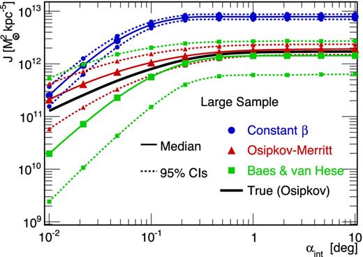
Median values (solid lines with symbols) and 95 per cent CIs (dotted lines with symbols) of J(αint) for a mock dSph (large sample) generated with an Osipkov–Merritt velocity anisotropy. The true J(αint) is given in solid black. The J-factor has been reconstructed using different anisotropy prescriptions: (i) constant (blue circles), (ii) Osipkov–Merritt (i.e. the correct parametrization, red triangles) and (iii) Baes & van Hese (more general than Osipkov–Merritt, green squares). See Sections 5.3 and 5.4.
5.4 Recommended option: |$\beta _{\rm ani}^{\rm Baes}$| analysis
In light of the previous result, when kinematic samples are large, it is important to have an as general as possible model for the anisotropy profile parametrization. Indeed, for real data, the true model for the anisotropy profile is obviously unknown. The Baes and van Hese model (four free parameters) is a good option since it encompasses both the constant and Osipkov–Merritt anisotropy profiles.
As shown in Fig. 8, the CIs of the J-factors are then larger using |$\beta _{\rm ani}^{\rm Baes}$| (green squares) because of the extra degrees of freedom in the parametrization. The analysis on the 32 models in Fig. 9 (distribution of Jmedian/Jtrue at αc) also shows that the use of Baes and van Hese profile (red solid line) can reduce biases coming from the wrong anisotropy parametrization, except for small samples where once again the statistical errors on σp dominate the error budget.
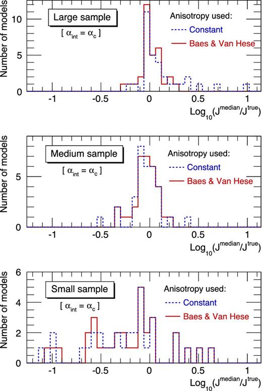
Distribution of the Jmedian/Jtrue at the critical integration angle αc using either a constant (blue dashed line) or a Baes and van Hese (red solid line) anisotropy profile, for the three sample sizes of the 32 Gaia Challenge models. The analysis of the mock ultrafaint samples (bottom panel) is dominated by the uncertainties on the σp data, and hence are not sensitive to a wrong choice of the anisotropy profile. This is no longer the case for mock classical samples (small effect, middle panel), and crucial for the ideal case of a large sample (top panel).
At worst, using |$\beta _{\rm ani}^{\rm Baes}$| increases the J-factor uncertainty by ∼2 for mock classical dSphs compared to using a simpler anisotropy model, but it can avoid biases for some models. We therefore recommend the use of the Baes and Van Hese parametrization for the velocity anisotropy.
6 IMPACT OF THE LIGHT PROFILE
Another key ingredient of the Jeans analysis is the light profile, which appears both in its projected I(R) and deprojected form ν(r) in the computation of the velocity dispersion (equation 6). A parametric model is usually fitted to the observed projected light profile, and then deprojected using the inverse Abel transform (see Section 2.1). In most dSph studies, Plummer or King profiles are fitted to the surface brightnesses (Strigari et al. 2008; Martinez et al. 2009; Walker et al. 2011), but exponential and Sérsic profiles (Section 2.1.2) are also often used (e.g. Irwin & Hatzidimitriou 1995; Łokas 2001). We now investigate the impact of such parametrizations on the reconstruction of the J-factor. A preliminary (and less systematic) study of this effect was performed in Charbonnier et al. (2011) – see their Appendix H.
The free parameters of the analysis are the Einasto DM profile parameters, using the optimal priors of Table 1. The light profile parameters are fitted separately, as described below, and the anisotropy parameters are fixed to their true values in order to be more sensitive to the effects of the light profile.
6.1 Subset of models and fit of the light profile
To avoid heavy computation, we select a subset of 3 ‘representative’ spherical models from The Gaia Challenge (second column of Table 2), chosen according to their Jmedian/Jtrue(αc) value obtained in the previous section: one close to 1, and two extreme models (maximal and minimal value).
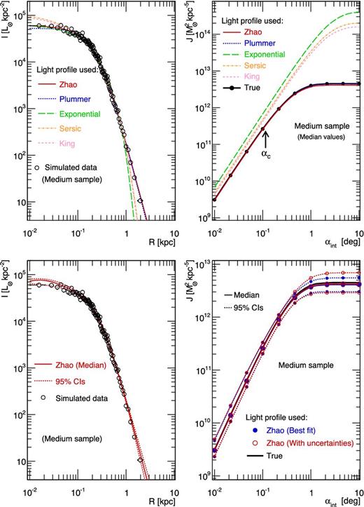
Top panels: best-fitting models of the surface brightness I(R) for the five light-profile parametrizations given in Section 2.1.2 (left); J(αint) obtained when using each of the five best-fitting light profile in the Jeans modelling (right) – see Section 6.1. Bottom panels: Zhao median surface brightness and its uncertainties (left) and propagation of these error bars to J(αint) (right). The same mock dSph galaxy (with medium-size velocity-dispersion sample) has been used in all panels.
6.2 Impact of different light-profile assumptions
For the three models and three sample sizes, we fit five different light profiles (Plummer, Zhao, exponential, Sérsic and King, see Section 2.1.2) to the surface brightness, using the likelihood function of equation (23). For one of the models, we show in the top panel of Fig. 10 the best fits obtained for the medium-size sample. For this model, the true light profile (Zhao) is very close to a Plummer profile (γ★ = 0.1 and β★ = 5), and Zhao (solid red) and Plummer (dotted blue) parametrizations provide an excellent fit to the data. The three other parametrizations significantly undershoot the data at large radii (top left panel), with both King and Sérsic also overshooting in the inner parts.
We then run our Jeans/MCMC analysis using each light-profile best fit. The top right panel of Fig. 10 shows the median J-factor obtained with the Jeans/MCMC analysis done with each of these best-fitting light profiles, compared to the one obtained with an analysis run with the true light profile (black solid line). Models that fit well the light profile (Zhao and Plummer) lead to a reconstruction of the J-factor as good as the one obtained when using the true light profile. With the three others, the J-factors systematically overshoot the latter: the CIs are not shown (for legibility purposes), but they encompass this reference J-value only at small integration angles (αint < 0.1, which corresponds to the optimal integration angle αc of that particular model). There is up to a factor of ∼3 systematic bias below αc, which increases to ∼100 at large angles. Here, we are showing the most pathological model of the three that have been studied, but the effect is always present, though less pronounced, for the two other models. A similar bias is obtained for mock ultrafaint dSph galaxies, but their J-factor CIs (not shown) are larger and therefore encompass this bias.
This shows that the light-profile parametrization plays a significant role in the J-factor reconstruction. It is therefore of particular importance to both measure and fit precisely the surface brightness profiles of dSph galaxies. We advocate the use of models with large degrees of freedom (e.g. Zhao), in order to obtain the best possible fits to the data and reduce biases in the derived J values.
6.3 Propagation of the light-profile uncertainties on J
Once a flexible-enough parametrization is selected (here a Zhao profile) for fitting the surface brightness, the uncertainties on the fit must be propagated to the J-factor.
We use our MCMC engine to recover both the median and CIs of the light profile, as illustrated in the bottom left panel of Fig. 10. Once done, we perform the standard Jeans/MCMC analysis, where, for each new step, a random point of the previously built light-profile chains is chosen: this effectively propagates the surface brightness profile uncertainties to the posterior distributions of the DM and anisotropy parameters.
For any sample size, we find that the small light-profile uncertainties only weakly affect the J-profile reconstruction, as shown in the bottom right panel of Fig. 10. This is emphasized by the comparison of the median value (solid lines) and CIs (dotted lines) obtained from the best-fitting light profile only (blue filled circles), or including the propagation of the error on the latter (red empty circles). Since the implementation of these errors is quite straightforward in the MCMC analysis, we nonetheless encourage their inclusion in the analysis when dealing with real data.
7 GEOMETRICAL EFFECTS: DM HALO TRIAXIALITY
In the spherical Jeans analysis, it is assumed that the stellar component is spherical, while it is known that dSphs have non-zero flattening (Irwin & Hatzidimitriou 1995; Walker 2013). The DM halo is also considered spherical, but cosmological N-body simulations have shown that both isolated DM haloes and their substructures have triaxial shapes (Frenk et al. 1988; Bailin & Steinmetz 2005; Bett et al. 2007; Muñoz-Cuartas et al. 2011).
Hayashi & Chiba (2012) have used an axisymmetric version of the Jeans equation in order to assess the impact of non-sphericity on the mass reconstruction. However, most studies rely on the spherical Jeans equation. In this section, we quantify the biases introduced by using a spherical Jeans analysis on triaxial DM haloes.
7.1 Triaxial haloes: description and analysis
The geometry of triaxial haloes is described by three principal axes a, b and c, with a ≥ b ≥ c and abc = 1. Kuhlen, Diemand & Madau (2007) found using the Via Lactea simulation (Diemand, Kuhlen & Madau 2007) that for dSphs-like sub-haloes, the ratios b/a and c/a are in average equal to 0.83 and 0.68, respectively, and using the Aquarius simulation (Springel et al. 2008), Vera-Ciro et al. (2014) found ratios close to 0.75 and 0.6. These objects appear therefore to be mildly triaxial, and simulations predict more triaxiality for more massive haloes (Schneider, Frenk & Cole 2012).
Mock data. For the analysis, we use the two triaxial mock dSphs made available by The Gaia Challenge (third column of Table 2, see also Section 2.4). We recall that each model consists of a triaxial stellar distribution embedded in a triaxial DM halo, with b/a and c/a ratios of 0.8 and 0.6, respectively, for both stellar and DM distributions. The velocity anisotropy profile of the stars is Baes and van Hese for both models, and the light and DM profiles have Zhao parametrizations. The only difference between the two models is the DM profile, which is cusped for one (γ = 1) and cored for the other (γ = 0.23).
Analysis steps. As described in Section 2.4, we once again create three sample sizes for each model, mimicking ultrafaint, classical and ideal dSphs. For each sample size, we build binned velocity-dispersion and binned light profiles for three different l.o.s., chosen along the three principal axes of the object. This allows us to investigate the effect of the different orientations in the reconstruction of the J-factor.
7.2 Projection effects
Triaxiality implies projection effects on both the observed stellar component and the DM profile. This depends on the unknown orientation of the haloes with respect to the observer l.o.s.
Impact on J factor true values. Fig. 11 shows the J-factor true values obtained for the cusp (red) or the core (blue) dSph for three l.o.s. orientations: along the short (solid), medium (dashed) and long (dotted) axes. First and as expected, the cuspy DM profile gives larger J values than the core. The projection effect on J reaches at most a 30 per cent difference at very small integration angles, for these mildly triaxial mock data.
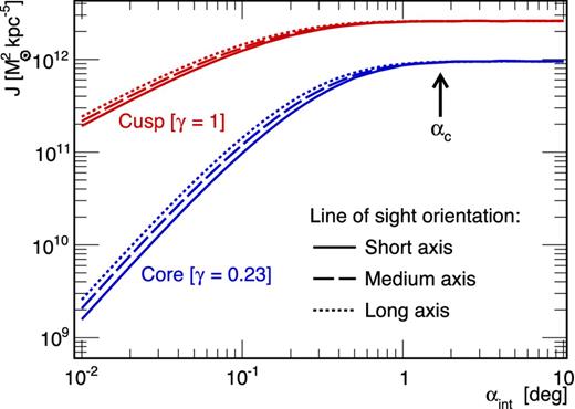
J-factor true values for the cusp (red) and core (blue) mock triaxial dSph galaxies. The three curves correspond to the l.o.s. aligned with the short (solid), medium (dashed) or long (dotted) axes of the halo.
Impact on the velocity dispersion profile. Fig. 12 shows the velocity-dispersion profiles obtained for the large samples (in order to emphasize the effect) of the two models (left-hand panel for the core, right for the cusp), when looking either along the long axis a (black squares) or the short axis c (circles). The projection effects have a strong impact on the velocity dispersion: while the global shape of the profile is preserved, it is shifted to larger values when the l.o.s. alignment moves from the short to the long axis. This is expected to have a significant effect on the reconstruction of the J- and D-factors.
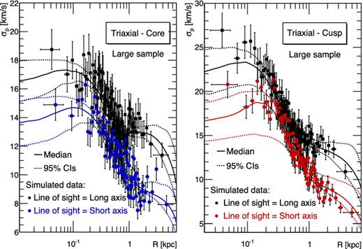
Projection effects (along short and long axis) on the reconstructed velocity-dispersion profiles (median and CIs in solid and dashed lines). The triaxial models shown are a core (left-hand panel) and cusp (right-hand panel), for a large-size sample.
7.3 Triaxiality-induced bias on J for a spherical Jeans analysis
We run our Jeans analysis on the two triaxial models, with all the findings of the previous sections (for the DM, anisotropy and light profiles, i.e. using the Einasto DM profile, Baes and van Hese anisotropy and Zhao light profile). It is performed for the three sample sizes and three orientations (the light profile is fitted separately for each orientation).
Fig. 13 shows the J-factors obtained for the mock classical cuspy dSph (similar results are obtained for the core profile), for l.o.s. oriented along the short (blue circles), medium (red triangles) and long axes (green squares). They are compared to the true value in black solid line (only the orientation along the intermediate axis is shown). A systematic shift appears between the three orientations, with the J-factor being maximum for the l.o.s. along the long axis. This is caused by the orientation-dependent velocity-dispersion profiles (shown in Fig. 12 for the large-size sample). At the optimal integration angle αc ≃ 1| $_{.}^{\circ}$|7, the reconstructed J-factors overshoot (or undershoot) the true values by a factor of ≲ 2.5. Some of the 95 per cent CIs (dotted lines) do not even encompass the true value for any integration angle.
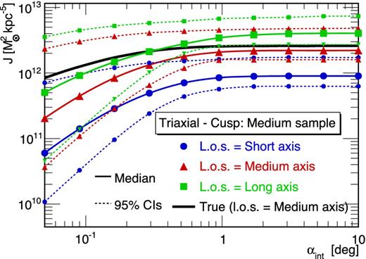
Median (solid lines) and 95 per cent CIs (dotted lines) J values reconstructed with the spherical Jeans analysis on a mock classical triaxial dSph (cuspy profile), for three l.o.s. orientations. The critical angle αc is the same as in Fig. 11.
Applying the spherical Jeans analysis to triaxial haloes therefore biases the J-factor reconstruction. The bias must be accounted for in the J-factor determination. We emphasize the fact that all observed dSphs display elliptical isophotes (Irwin & Hatzidimitriou 1995; Martin et al. 2008) and thereby violate the common assumption of spherical symmetry. This assumption can be relaxed, for example, in the axisymmetric Jeans models of Cappellari (2008), or in alternative techniques that rely on orbit-based modelling (Schwarzschild 1979) or made-to-measure models (Syer & Tremaine 1996; Long & Mao 2010). One disadvantage of these models is that their greater computational expense inhibits the range of systematic tests that can be performed in a reasonable amount of time. Nevertheless, we expect that the greater flexibility of such models can reduce the biases we found in tests against mock data drawn from triaxial models.
8 CONCLUSIONS
We have studied the impact of the different ingredients of the spherical Jeans analysis on the reconstruction of the astrophysical factors J and D (respectively for annihilating and decaying DM) of dSph galaxies. We find that the assumptions made regarding the ingredients of the analysis (DM, velocity anisotropy and light profiles; spherical symmetry) may significantly impact those quantities. Coupling the Jeans analysis to an MCMC engine and relying on a set of mock dSph galaxy data, we were able to quantify the biases (seen as trends for systematic offsets of the reconstructed median values from the true ones) and uncertainties (assessed by the width of the 95 per cent CIs) associated with each assumption, using three sizes of mock samples to mimic data sets of ultrafaint (small sample), classical (median sample) and ‘ideally observed’ (large sample) dSph galaxies. Table 4 summarizes the main findings of this study.
Summary of all effects discussed in the paper for annihilation and decay (J- and D-factors). The upper block corresponds to biases induced by the choices of parametrization and halo triaxiality. The lower block gives the minimum (maximum knowledge) and typical (|$\rho _{\rm DM}^{\rm Einasto}$|+ |$\beta _{\rm ani}^{\rm Baes}$| modelling) uncertainties expected in a data-driven Jeans analysis. Note that we show the quantity |$J^{\pm 95\,\mathrm{per cent}\, \rm CI}/J^{\rm median}$| instead of |$J^{\pm 95\,\mathrm{per cent}\, \rm CI}/J^{\rm true}$| (presented in Figs 4 and 7), in order to be comparable to the expectations of real data analyses.
| Section | Annihilation | Decay | Comments | |||||
|---|---|---|---|---|---|---|---|---|
| Ultrafaint | Classical | Ideal | Ultrafaint | Classical | Ideal | |||
| Bias from: | |$J^{\rm median}/J^{\rm true} (\alpha _{c}^{J})$| | |$D^{\rm median}/D^{\rm true}(\alpha _{c}^{D})$| | ||||||
| Einasto versus Zhao | Section 4.2 | none | none | none | none | none | none | → use Einasto + cutsa |
| Wrong βani | Section 5.3 | none | ≲ 3 | ≲ 10 | none | ≲ 2.5 | ≲ 2 | → use |$\beta _{\rm ani}^{\rm Baes}$| |
| Wrong Ilight | Section 6.2 | ≲ 2 | ≲ 3 | ≲ 3 | ≲ 1.5 | ≲ 4 | ≲ 4 | → use Zhao |
| Triaxiality | Section 7.3 | ≲ 2.5 | ≲ 2.5 | ≲ 2.5 | ≲ 2 | ≲ 2 | ≲ 2 | Systematic uncertainty |
| Uncertaintiesb: | |$J^{\pm 95\,\mathrm{per cent}\, \rm CI}/J^{\rm median} (\alpha _{c}^{J})$| | |$D^{\pm 95\,\mathrm{per cent}\, \rm CI}/D^{\rm median}(\alpha _{c}^{D})$| | ||||||
| Maximum knowledge | Section 4.3 | ≲ 20 | ≲ 2 | ≲ 1.5 | ≲ 8 | ≲ 1.5 | ≲ 1.25 | DM only + cutsa |
| |$\rho _{\rm DM}^{\rm Einasto}$|+ |$\beta _{\rm ani}^{\rm Baes}$| modelling | Section 5.4 | ≲ 20 | ≲ 4 | ≲ 2.5 | ≲ 10 | ≲ 2 | ≲ 2 | – |
aEnforce |$r_{s} \ge r_{s}^{\star }$| and α ≥ 0.12 in the priors.
bLight-profile uncertainties have a very small effect on J and D at αc, and are not shown here.
Impact of the various ingredients on J- and D-factors
DM profile: given the precision and the small spatial range covered by velocity-dispersion measurements, we find that it is equivalent to use a Zhao or an Einasto DM parametrization in the Jeans analysis. We recommend the use of the Einasto profile as the smaller number of parameters produces less degeneracies and faster MCMC analyses than for the Zhao case. To avoid extremely large upper limits (up to factors of ∼106 for |$J^{+95\,\mathrm{per\ cent}\ \rm CI}/J^{\rm median}$| of mock ultrafaints), coming from the sampling of unrealistic models, it is necessary to put weak priors on the scale radius and slope of the Einasto profile, namely |$r_s\ge r_s^\star$| and α ≥ 0.12;
Velocity anisotropy profile: making the wrong assumption on the anisotropy profile parametrization can lead to strongly biased astrophysical factors (with median J values up to factors of a few above or below the true values depending on the sample size, with the 95 per cent CIs not encompassing the true values). Instead of using a constant anisotropy profile (as done in many studies), we recommend the use of a flexible profile such as that of Baes & van Hese. The latter encompasses both the constant and Osipkov–Merritt profiles, and its four parameters allow for more flexibility in the fit.
Light profile: using the wrong light-profile parametrization can lead up to a factor ≳ 10 bias (of the astrophysical factor) at large integration angles αint ≳ αc, and ∼3 below. We recommend the use of a Zhao profile for the light as it appears a good choice to fit the generally well-sampled light profiles. Propagating the errors on the light profile to the astrophysical factor makes no significant difference as these errors are always much smaller compared to other uncertainties, regardless of the sample size.
Triaxiality: the last important effect investigated is the use of a spherical analysis on DM haloes that are likely to be triaxial. First, even with a perfectly known DM profile, projection effects lead to a ∼30 per cent systematic effect, depending on the DM halo orientation with respect to the l.o.s. (for αint ≲ αc). Second, projection effects in the velocity-dispersion data lead to J and D values that can undershoot or overshoot the true value by a factor of a few. This systematic effect must be accounted for separately in the error budget, since the orientations of the dSph galaxies remain unknown.
When all these effects are taken into account, we confirm that (i) the inner slope of DM profiles for dSph galaxies is not well constrained by the Jeans analysis, even when the well-known velocity anisotropy–mass degeneracy is broken; (ii) the astrophysical factor can nonetheless be well constrained; and (iii) the critical angle (for which the uncertainty is the smallest) found for the J-factor also exists for the D-factor, with |$\alpha _{c}^{D} \approx r_{s}^{\star }/d = \alpha _{c}^J/2$|.
Conclusions for the different sample sizes
Ultrafaint dSph galaxies: these objects are the most promising dSph galaxy targets for indirect detection as some of them are found very close to us (∼20–40 kpc). However, they are also the most uncertain because of the few kinematic data available. In order to obtain the best constraints on these objects in a ‘data-driven’ analysis, a cut on the prior of the scale radius (|$r_s\ge r_s^\star$|) is mandatory. The statistical uncertainties linked to the sparsity of the data always dominate the error budget, regardless of the Jeans modelling (anisotropy, light and DM profile parametrizations): we typically find J±95 percent CI/Jmedian ≲ 20 at αint = αc, and ≲ 100 at 0.1αc and 10αc.
Classical dSph galaxies: these objects have already been analysed in a similar framework in Charbonnier et al. (2011). The analysis of this paper goes further, with several new identified sources of biases and uncertainties. On the one hand, the cuts on the priors were not all included in Charbonnier et al. (2011), so that the CIs obtained by these authors may be slightly overestimated. On the other hand, the use of more generic anisotropy and light profiles, and the systematic effect of triaxiality may slightly shift and increase these errors. A re-analysis is required to obtain better estimates on real data. In any case, typical uncertainties on the 95 per cent CIs for these objects are J±95 percent CI/Jmedian ≲ 4 at αint = αc, and ≲ 10 at 0.1αc and 10αc.
‘Ideally observed’ dSph galaxies: future instruments may provide much more precise and numerous kinematical data, if the observed objects contain enough stars (which is the ultimate limitation). If this is the case, halo triaxiality will need to be handled by non-spherical Jeans analyses (see e.g. Hayashi & Chiba 2012) as it will then become the main source of bias in the spherical Jeans analysis. The main source of uncertainty in this ideal case is the velocity anisotropy profile. Higher order Jeans analyses will probably appear as very helpful tools for reducing these uncertainties (see e.g. Richardson & Fairbairn 2013, 2014; Richardson et al. 2014). However, we have found that even in the context of a maximum knowledge analysis (i.e. with the light profile and velocity anisotropy perfectly known), the best that can be achieved is J±95 percent CI/Jmedian ≲ 1.5 at αint = αc, and ≲ 2.5 at 0.1αc and 10αc.
Suggestions and future studies.
The use of mock data has led to the determination of an optimal strategy to obtain the least biased and best constrained results on the astrophysical factors. In the context of ‘data-driven’ spherical Jeans analyses, we recommend the use of the Einasto DM profile (with |$r_s\ge r_s^\star$| and α ≥ 0.12), the Baes and van Hese velocity anisotropy profile, the Zhao profile for the light, and accounting for a possible systematic bias from triaxiality. In a forthcoming article, we will analyse all dSph galaxy data available to us using this optimal setup (in preparation).
We thank the anonymous referee for his careful reading of the manuscript that led to many useful improvements. We are very grateful to M. I. Wilkinson for allowing us to use the mock data from Charbonnier et al. (2011). VB would like to warmly thank L. Derome and A. Putze for their help using and interfacing the GreAT package and for the useful discussions about the MCMC. This work has been supported by the ‘Investissements d'avenir, Labex ENIGMASS’. This study used the CC-IN2P3 computation centre of Lyon.
Parameters with subscript ‘★’ refer to 3D stellar density profiles that take the same functional form as equation (8). For each suite, the DM profile is Zhao.
Caution is required when interpreting the histogram in Fig. 4. It should not be used to infer what the mean upper 95 per cent CI should be, as the distribution of the profiles in the mock dSph sample may not be representative of the (unknown) Milky Way's dSph galaxies profile distribution. However, it clearly shows the benefit of the cut |$r_s \ge r_s^\star$| on a sample presenting a large variety of DM profiles, and that is expected to encompass the range in which actual Milky Way's dSph profiles lie.
There is no direct equivalency between the inner slope of the Zhao profile and the logarithmic slope of the Einasto profile dlog ρ/dlog r = −2(r/r−2)α. The lower limit on α is chosen so that the logarithmic slope is equal to −1 for r/r−2 = 1/300, leading to α ∼ 0.12. The value α = 0.05 used for the base prior of Table 1 corresponds to a logarithmic slope of −1.5 for the same value of r/r−2.
REFERENCES
APPENDIX A: MCMC OPTIMIzATION
Our MCMC analysis relies on a multivariate Gaussian proposal function. We recall that the closer to the proposal function the target distribution, the better the MCMC efficiency. The latter is defined as the ratio between the number of accepted points (after taking into account the burn-in and correlation lengths) and the number of computed points.
Fig. A1 shows the correlations and PDFs of the three parameters describing the Einasto DM profile, for a maximum knowledge analysis on a mock classical dSph galaxy. The two panels correspond to the output of two MCMC runs, based on two different combinations of the Einasto parameters. Using {log10(ρ−2), log10(r−2), α} (left-hand panel) leads to strongly correlated parameters, with long tails for both ρ−2 and r−2, hence a rather poor efficiency (∼6 per cent). Using |$\left\lbrace \log _{10}(\rho (r_{s}^{\star })), \log _{10}(r_{-2}), \alpha \right\rbrace$| instead increases the efficiency almost threefold (∼16 per cent): the DM density is actually best constrained at |$r = r_{s}^{\star }$| (see also Fig. 2), and the variable |$\log _{10}(\rho (r_{s}^{\star }))$| is close to be Gaussian distributed (top right panel of Fig. A1). Note that this second combination of parameters can also be made for a Zhao DM profile.
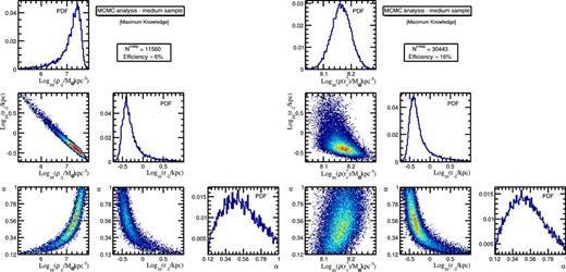
Correlations and PDFs of three parameters describing the Einasto DM profile, for a maximum knowledge run on a mock classical dSph. Left-hand panel: MCMC analysis with the combination of parameters {log10(ρ−2), log10(r−2), α}, with the priors and cuts of Table 1. Because of the non-Gaussianity, the efficiency is rather poor (∼6 per cent). Right-hand panel: MCMC analysis with the combination of parameters |$\left\lbrace \log _{10}(\rho (r_{s}^{\star })), \log _{10}(r_{-2}), \alpha \right\rbrace$|. The first parameter is now approximately Gaussian, and the correlations are much weaker. The efficiency is significantly larger (∼16 per cent).
The prior used here for |$\log _{10}(\rho (r_{s}^{\star }))$| is similar to the one we used on log10(ρ−2): it is flat within the range [5, 13]. We have checked that using this prior as well as the usual priors of Table 1 on log10(r−2) and α, we recover a flat distribution on log10(ρ−2). Therefore, these two combinations of parameters lead to the same prior distributions, and give the same results.
We have focused in this study on the use of uniform priors, but there is actually no clear answer regarding the best choice of prior distribution. It can however have a strong impact on the results, particularly for ultrafaint dSphs for which the data constrain only weakly the physical parameters.
APPENDIX B: OPTIMAL INTEGRATION ANGLE FOR J AND D
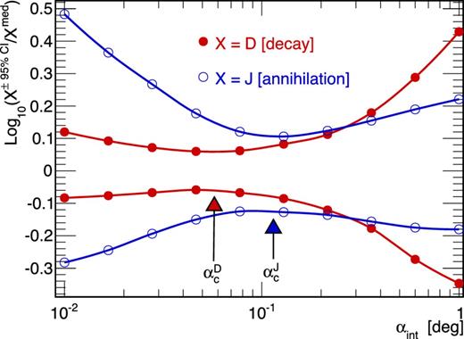
Ratio |$X^{\pm 95 \,\mathrm{per cent}\, \rm CI}/X^{\rm median}$| for annihilating DM (X = J, blue empty circles) and decaying DM (X = D, red filled circles). The arrows show the position of the optimal angles |$\alpha _{c}^J$| (equation (B1)) and |$\alpha _{c}^D$| (equation (B2)), for this peculiar mock classical dSph galaxy. These angles coincide with the pinch of the CIs for which the uncertainty on X is minimized.
APPENDIX C: IMPACT OF ANISOTROPY PARAMETRIZATION ON THE DARK MATTER DENSITY PROFILE AND MASS RECONSTRUCTION
This appendix further explores the impact of using the wrong velocity anisotropy parametrization on the DM density profile and mass reconstruction. We refer the reader to Section 5.3 for the details of the analysis. We show in Fig. C1 the velocity-dispersion profile (left), the DM density profile (middle) and the PDFs and correlation (right) of the mass at r = 300 pc M300 and of ρ−2, for two typical mock classical dSph galaxies. In the top row, the model follows an Osipkov–Merritt parametrization while in the bottom row the model has a constant anisotropy. In each case, the Jeans analysis is run using either a constant or an Osipkov–Merritt anisotropy.
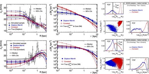
Velocity-dispersion profile (left), DM density profile (middle) and PDFs of M300 (mass at r = 300 pc) and ρ−2 (right), reconstructed for a mock cored classical dSph galaxy with an Osipkov–Merritt (top) or a constant (bottom) velocity anisotropy. For each model, the Jeans analysis is run using either an Osipkov–Merritt (blue) or a constant (red) anisotropy. Both give similar fits to the velocity-dispersion profiles, but using the wrong anisotropy profile leads to strong biases on both the DM density profile and the mass at 300 pc.
The fit to the velocity-dispersion profile (Fig. C1, left) is always satisfactory, whether we use the right anisotropy parametrization or not. However, the effect on the reconstructed DM density profile (middle) can be very strong. For example, using a constant anisotropy for the model with an Osipkov–Merritt anisotropy (Fig. C1, top row – middle column, red empty circles) leads to a cuspy DM density profile, whereas the true profile is a core (black solid line). When we look at the PDFs (top row – right column), we see the distinct populations arising from using either a constant (red) or an Osipkov–Merritt (blue) profile. The effect is a bit less pronounced for the model with a constant anisotropy (bottom panels).
Using the wrong anisotropy parametrization can therefore produce strong biases on the DM density profile, that in turns, impact both the J- and D-factors but also the estimated mass of the object. Using a Baes and van Hese anisotropy profile allows us to mitigate this effect (see Section 5.3).
APPENDIX D: RESULTS FOR D-FACTORS (DECAYING DM)
Many DM models correspond to stable particles, thermally produced in the early Universe. DM could also consist of unstable long-lived particles, the decay of which could generate γ or X-rays, via prompt and inverse Compton emissions (Ibarra, Tran & Weniger 2013). In this scenario, exotic signals have been looked for in the Milky Way (Cirelli, Panci & Serpico 2010), in M31 (Boyarsky et al. 2008), in clusters of galaxies (Dugger, Jeltema & Profumo 2010; Cirelli et al. 2012; Combet et al. 2012) and in dSphs (Essig et al. 2009; Acciari et al. 2010; Aliu et al. 2012) using data sets from various instruments (Fermi-LAT, Imaging Air Cherenkov Telescopes (IACTs), XMM–Newton). Non-detections have led to constraints on the lifetime τ of the decaying DM particle. Note however that an exotic X-ray line at 3.5 keV has recently been identified in M31 and in clusters of galaxies, that could originate from DM decay (Boyarsky et al. 2014; Bulbul et al. 2014). As in the case of annihilation, a careful estimation of the astrophysical D-factors and of their uncertainties are required in order to derive those constraints.
The astrophysical D-factor corresponds to the integration along the l.o.s. of the DM density (where the J-factor requires the DM density squared). Compared to the J-factor, the D-factor is therefore less sensitive to the uncertainties on the DM density profile. In this appendix, we briefly review the impact on the D-factor of the different effects discussed in the body of this paper.
DM modelling: maximum knowledge setup
Optimal cut|$r_{s} \ge r_{s}^{*}$|. The effect of this cut is less pronounced for the D-factor than for the J-factor: for mock ultrafaint dSphs, it slightly reduces the upper CIs at small integration angles, and the lower CIs at large angles. This is shown, for a typical model, in the bottom right panel of Fig. 2. As for the J-factor, this cut is always applied for the D-factor determination.
Zhao versus Einasto. Similarly to J-factors, using an Einasto or a Zhao DM parametrization gives very comparable D-factors. Fig. D1 shows the D-factor obtained using either a Zhao (blue filled circles) or an Einasto (red empty circles) profile, for a mock classical dSph galaxy (maximum knowledge setup); similar results for median and CI values are found in the two cases.
Sample size. The size of the sample also plays a major role in the D-factor uncertainties. The D-factors are less sensitive to the DM profile uncertainties than the J-factors, and are more tightly constrained. Using the D+95 percent CI/Dtrue values obtained for the 64 models from Walker et al. (2011) (see Table 2), the D-factor relative uncertainty at |$\alpha _{c}^{D}$| is found (not shown) to be at most ∼1.5 (resp. ∼8) for the mock classical (resp. ultrafaint) dSph galaxies, while the corresponding J-factor uncertainty is at most ∼3 (resp. ∼25).
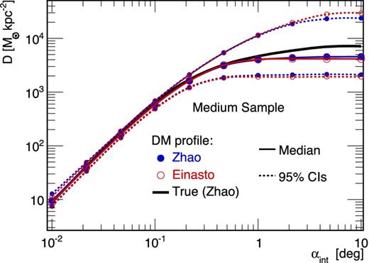
D-factor median values (solid lines with symbols) and 95 per cent CIs (thin dashed lines with symbols) for a mock classical dSph galaxy. MCMC/Jeans analyses with a Zhao (blue filled circles) or a Einasto (red empty circles) DM profile give similar results, as for the J-factor.
Anisotropy profile
Optimal cut α ≥ 0.12. We found in Section 5 that when a constant velocity anisotropy is free to vary in the Jeans analysis, the cut α ≥ 0.12 on the Einasto shape parameter significantly reduces the uncertainties on the J-factor. For the D-factor, the cut has no strong effect: this quantity is less sensitive to the steepness of the DM profile in the inner parts. Nevertheless, for consistency with the J-factor reconstruction, we also implement this cut for D-factor calculations.
|$\beta _{\rm ani}^{\rm Cst}$|versus|$\beta _{\rm ani}^{\rm Osipkov}$|. Results similar to the J-factor ones are found when using the wrong anisotropy profile parametrization: the D-factor reconstruction can be strongly biased. We show in Fig. D2 the D-factor obtained for a mock dSph (large sample) generated with an Osipkov–Merritt anisotropy, using either a constant (blue circles) or an Osipkov–Merritt (red triangles) model in the Jeans analysis. The reconstructed D-factor is compatible with the true one (black solid line) only when the right parametrization is used.
|$\beta _{\rm ani}^{\rm Baes}$|analysis. Using the more general Baes and van Hese anisotropy profile (equation 18) allows us to mitigate these biases for medium and large samples. This profile leads to larger CIs (typically, they are ∼25 per cent larger at αc), but less biased median values, as shown in green squares in Fig. D2. For mock ultrafaint dSph galaxies, the D-factors obtained with the three anisotropy profiles used here are compatible. We also advocate the use of this general parametrization for the D-factor determination.
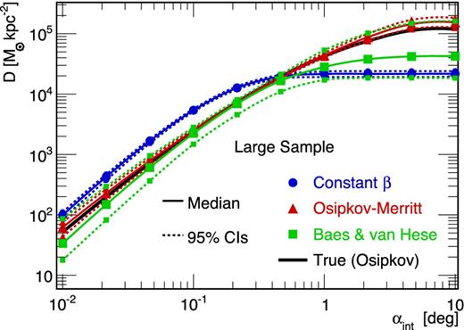
Median values (solid lines with symbols) and 95 per cent CIs (dotted lines with symbols) of D(αint) for a mock dSph (large sample) generated with an Osipkov–Merritt velocity anisotropy. The true D(αint) is given in solid black. The D-factor has been reconstructed using different anisotropy prescriptions: (i) constant (blue circles), (ii) Osipkov–Merritt (i.e. the correct parametrization, red triangles) and (iii) Baes and van Hese (green squares).
Light profile. The conclusions reached in Section 6.1 for J-factors hold for D-factors: the light-profile parametrization plays a significant role in the D-factor reconstruction, whereas propagating the light-profile uncertainties has a weak effect only. This is illustrated in Fig. D3, for the same model as in Fig. 10: we show the D-factors obtained for a mock classical dSph galaxy using the five different light-profile parametrizations of Section 6.1 (left-hand panel), as well as the effect of propagating the light-profile uncertainties (right-hand panel). For a Jeans analysis dedicated to D-factor determination, we therefore advocate the use of a very general light-profile parametrization.
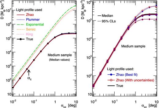
Left-hand panel: D(αint) obtained when using each of the five best-fitting light profiles in the Jeans modelling – see Section 6.1. Right-hand panel: propagation to D(αint) of the uncertainties on a Zhao light-profile fit. The same mock dSph galaxy (with medium-size velocity dispersion sample) has been used for the two plots.
DM halo triaxiality
Projection effects. For a triaxial halo, the l.o.s. orientation with respect to the principal axes of the halo plays a role when computing the true D-factor, just as for the J-factor. The same 30 per cent difference (shown in Fig. 11 for J, not repeated here) appears at very low integration angles depending whether the l.o.s. is aligned with the short or the long axis of the halo.
Triaxiality-induced bias. Fig. D4 shows the D-factors reconstructed for a mock classical (cuspy) dSph galaxy, with the short (blue circles), medium (red triangles) and long axis (green squares) aligned along the l.o.s. They are compared to the true value in black solid line (for the intermediate axis l.o.s. orientation). The same systematic shift as observed for the J-factors (Fig. 13) appears between the three D-factors, due to projection-induced effects of the velocity-dispersion profiles (Fig. 12). Factors of ∼2 systematic uncertainties must then be accounted for in the D-factor determination.
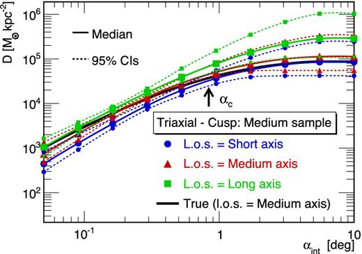
Median (solid lines) and 95 per cent CIs (dotted lines) D values reconstructed with the spherical Jeans analysis on a mock classical triaxial dSph galaxy (cuspy profile), for three l.o.s. orientations.
