Developing a model for neutron star oscillations following starquakes

Keer, L.; Jones, D. I.

doi:10.1093/mnras/stu2123

Abstract

Glitches – sudden increases in spin rate – are observed in many pulsars. One mechanism advanced to explain glitches in the youngest pulsars is that they are caused by a starquake, a sudden rearrangement of the crust of the neutron star. Starquakes have the potential to excite some of the oscillation modes of the neutron star, which means that they are of interest as a source of gravitational waves. These oscillations could also have an impact on radio emission. In this paper, we make upper estimates of the amplitude of the oscillations produced by a starquake, and the corresponding gravitational wave emission. We then develop a more detailed framework for calculating the oscillations excited by the starquake, using a toy model of a solid, incompressible star where all strain is lost instantaneously from the star at the glitch. For this toy model, we give plots of the amplitudes of the modes excited, as the shear modulus and rotation rate of the star are varied. We find that for our specific model, the largest excitation is generally of a mode similar to the f-mode of an incompressible fluid star, but that other modes of the star are excited to a significant degree over small parameter ranges of the rotation rate.

asteroseismology, gravitational waves, stars: neutron, pulsars: general

1 INTRODUCTION

Neutron stars normally rotate at an extremely regular rate. Once the steady slowdown over time from magnetic dipole radiation is accounted for, pulsars can keep time to an accuracy of one part in 10¹¹ or more (Lyne & Graham-Smith 1998). However, younger pulsars often display more erratic behaviour. Some of this variation comes from timing noise, small unmodelled deviations in the pulse period. More dramatically, many have been observed to undergo a sudden speed-up in rotation rate, known as a glitch.

Glitch observations are discussed in detail in Espinoza et al. (2011), where glitching pulsars are shown to exhibit a diverse range of behaviours. The size of a glitch can be characterized by the fractional change in spin frequency |$\frac{\Delta \Omega }{\Omega }$| of the pulsar. Glitches have been observed spanning the range |$\frac{\Delta \Omega }{\Omega }\sim 10^{-11}-10^{-5}$|⁠, and the distribution of glitch sizes experienced by an individual pulsar also varies widely. Some pulsars, such as the Vela, undergo ‘giant’ glitches of approximately regular size with |$\frac{\Delta \Omega }{\Omega }\sim 10^{-6}$|⁠, whereas some of the youngest pulsars such as the Crab have smaller glitches with |$\frac{\Delta \Omega }{\Omega } \lesssim 10^{-8}$|⁠, and glitch sizes are distributed over a wide range (Wong, Backer & Lyne 2001).

Glitches are likely to excite oscillation modes of the star, making them an interesting candidate source for gravitational wave emission. These oscillations could also be expected to shake the star's magnetosphere, leading to the possibility of radio emission observable by next generation radio telescopes. The increased sensitivity and time resolution of the Square Kilometre Array may allow the glitch event to be detected directly.

However, the nature and amplitude of the oscillation modes excited will depend strongly on the mechanism producing the glitches, which is as yet unknown. The leading explanation for the larger glitches is that they are caused by a rapid transfer of angular momentum from the superfluid component of the star to its crust (Anderson & Itoh 1975). This superfluid component may ordinarily be only weakly coupled to the crust, which gradually slows down through magnetic braking. This is because the superfluid can only slow down through the outward migration of its quantized vortices. As they reach the solid crust they may become pinned to the nuclei in the crystal lattice, fixing the angular momentum of this part of the superfluid. A glitch would then be triggered by an event that could increase the coupling between the two components by producing a sudden collective unpinning of these vortices. Various mechanisms for this unpinning have been proposed (Alpar et al. 1984; Melatos, Peralta & Wyithe 2008; Glampedakis & Andersson 2009).

Another idea is that glitches are produced by a starquake – a sudden rearrangement of the crust of the star (Baym & Pines 1971). This model uses the fact that while a fluid star would be able to freely adjust its shape as the neutron star slows down over time, the solid crust of a neutron star will resist the deformation from its relaxed state; consequently, it will stay more oblate than a fluid star would. The level of strain in the crust builds up, and this may reach a critical value at which the crust can no longer withstand the strain and breaks. The release of strain means that the star loses some of its residual oblateness. The moment of inertia decreases, and so by conservation of angular momentum there must be a corresponding increase in the star's angular velocity, producing the observed glitch. This model is not able to produce a large enough energy release to account for the largest glitches, such as those of Vela (Alpar et al. 1996), but is still promising for describing smaller glitches such as those of the Crab.

The prospects for gravitational wave detection from the superfluid model have been discussed in papers by Sidery, Passamonti & Andersson (2010) and van Eysden & Melatos (2008). In this paper, we will concentrate on the starquake model, starting by making some order-of-magnitude estimates for the maximum energy released in a starquake, and the amplitudes of the oscillations produced, using a formalism originally developed by Baym & Pines (1971). We then develop a more detailed framework for calculating the oscillations excited by a glitch, based on calculating initial data for the glitch and projecting it against a basis of normal modes of the star. We carry this out for a toy model in which the star is completely solid and incompressible, and the glitch is modelled by an instantaneous loss of all strain. Although this acausal glitch mechanism is not realistic, it is a sensible starting point which allows us to develop the model, and even this simple model produces some interesting results.

We will start in Section 2 by giving an overview of our model for a starquake and fixing notation for the rest of the paper. In Section 3, we make order-of-magnitude estimates of the amplitude of oscillations produced by the quake, both for our specific model and for an optimistic scenario in which all energy released in the quake goes into oscillations. For this scenario, we also calculate the gravitational wave emission produced by the oscillation, both for an ordinary neutron star with a fluid interior and a solid quark star. We then move on to the more detailed model, describing the calculation of the initial data for the glitch in Section 4 and the normal modes of the rotating star in Section 5. In Section 6, we develop a projection scheme that allows us to calculate the amplitudes of the oscillation modes excited, and discuss the results of this. Section 7 then provides a summary of the results of the paper.

2 THE STARQUAKE TOY MODEL

In this section, we describe our simplified toy model for a glitch. This is illustrated in Fig. 1, where the main stages of the glitch are labelled as Stars A–D. We will work in Newtonian gravity throughout the paper. We will also only consider the case of slow rotation, in which rotation is treated as a perturbation about a spherical background star (Star S of the figure).

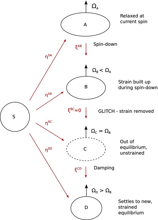
Figure 1.

Diagram of our starquake model. As the star spins down from an initial, relaxed configuration (Star A) spinning at angular velocity Ω_A, strain builds up in the crust. When this reaches a critical level (Star B) at some angular velocity Ω_B, the crust cracks and strain is removed. Immediately after the starquake the star is out of equilibrium (Star C), and oscillates briefly before settling down to a new equilibrium state (Star D) spinning with angular velocity Ω_D. We will treat the equilibrium states as perturbations about a spherical background configuration, Star S. The maps η track the displacements of particles in S to their new positions in Stars A–D, while the ξ displacement fields map between A and D.

Open in new tab Download slide

In this toy model, we take our star to be completely solid and incompressible: this will allow us to use analytic results for the equilibrium configurations of the rotating star, and for the normal modes of Star S. The star is also modelled as an elastic solid, so that it has some relaxed state of zero strain, and deformation from this state will induce a strain field in the star. This strain field is built from the displacement vector field |$\boldsymbol {\xi }$| connecting points of the star in its relaxed configuration to their new positions in its current configuration.

In our model, the star starts in an unstrained state, Star A, spinning with angular velocity Ω_A. In this relaxed state, the star will have the same shape as a completely fluid star. This star will then spin-down as it loses energy. This will cause it to become less oblate, inducing a strain field in the star as it is deformed from its relaxed configuration. The starquake then occurs at the point where the strain has built up to some critical level where the crust can no longer support it – we label this as Star B, which is spinning at some angular velocity Ω_B. The strain field at this point can be calculated from the displacement field that connects particles in the unstrained Star A to their new positions in Star B, which we will label |$\boldsymbol {\xi }^{{\rm AB}}$|⁠.

We now need to specify our model of the glitch itself. For our toy model, we will take the extreme case where all of the strain energy of Star B is lost from the star. More precisely: ‘We assume that all the strain is lost from the star at the glitch, so that the new, unstrained reference state of the star is that of Star B. Furthermore, we assume that this energy is just lost from the star as heat, rather than going into kinetic or gravitational energy. This means that the mass distribution of the star will not be changed at the glitch – particles in Star C immediately after the glitch are not displaced from their positions in Star B: using the same labelling method for the displacement field between Stars B and C, we have |$\boldsymbol {\xi }^{{\rm BC}} = 0$|⁠.’

After the glitch, the star will now be out of equilibrium (Star C), and so it will start to oscillate. These oscillations will be damped until the star finally reaches a new equilibrium configuration, Star D, with angular velocity Ω_D. This equilibrium state is deformed from its unstrained state, Star C, and so has some residual strain constructed from the displacement field |$\boldsymbol {\xi }^{{\rm CD}}$|⁠.

2.1 Plan of the calculation

The basic idea of our starquake model is to project initial data describing the starquake against the set of oscillation modes of the star after the glitch, in order to find the amplitudes of the excited oscillation modes. This process has three stages.

First we construct the initial data, which will take the form of a displacement field |$\boldsymbol {\xi }^{{\rm DC}}$| and velocity field |$\dot{\boldsymbol {\xi }}^{{\rm DC}}$| describing how particles in the star are perturbed from equilibrium after the glitch. Note that the initial data links the final state, Star D, to the state of the star before the glitch, so the displacement field initial data is in the opposite direction to the strain field |$\boldsymbol {\xi }^{{\rm CD}}$|⁠. This construction will involve finding the new equilibrium state of the star after the starquake, Star D, which is rotating with angular velocity Ω_D. We do this in the case of slow rotation, where the change in the star's equilibrium configuration due to rotation is treated as a perturbation about the spherical background star, Star S.
Next, we calculate the spectrum of oscillation modes of Star D. We will start by finding analytic results for the eigenvalues and eigenfunctions of the spherical Star S. We then introduce rotation as a perturbation and calculate the first-order corrections to these modes.
Finally, we can project our initial data, |$\boldsymbol {\xi }^{{\rm DC}}$| and |$\dot{\boldsymbol {\xi }}^{{\rm DC}}$|⁠, against this set of modes of Star D, to see which ones are excited by it. The eigenfunctions of Star S are orthogonal, which we show in Appendix B. However, once we include rotation, this is no longer the case. We describe a scheme that will nevertheless allow us to carry out the projection.

3 ENERGY ESTIMATES FOR THE MODEL

Before making any detailed calculations, we can get more insight into the starquake mechanism for glitches by making some estimates for the energy released by the quake. An estimate that has appeared in the literature (Abadie et al. 2011) takes the rotational kinetic energy available to the star and multiplies it by the fractional change in velocity characterizing the glitch, to obtain

\begin{equation} \Delta E \sim I\Omega ^2 \left(\frac{\Delta \Omega }{\Omega }\right). \end{equation}

(1)

However, the actual value of the change in energy will depend strongly on the detailed physics of the glitch. This in turn depends on the mechanism that triggers the glitch. Here we will concentrate on the starquake model, and make some estimates for the energy released in the glitch in this case, and the amplitude of the oscillations produced. We will use the notation of the previous section, where the stages of the starquake model are labelled by Stars A–D.

In the specific model outlined in the previous section, the strain energy is just lost from the star at the glitch. In this case, the energy available to go into oscillations comes only from the change in the star's gravitational and kinetic energy as it settles to a new equilibrium state. This is the energy difference between Stars C and D, ΔE_CD = E_C − E_D.

Although this is perhaps the simplest option to model, it is not necessarily the most realistic. We can also imagine taking the strain energy of the star before the glitch and putting some of it into, for example, the kinetic energy of the star after the quake (if the crust cracks or otherwise moves about).

The upper bound on this would be to put all the strain energy made available into gravitational or kinetic energy. This would correspond to the total energy immediately after the glitch being that of Star B. This gives us an upper limit on the energy available to go into oscillations at the glitch, ΔE_BD = E_B − E_D.

In this section, we will make an estimate for both the upper limit on energy released, ΔE_BD, and the energy released in our specific model, ΔE_CD. To do this, we will start by building on the starquake model of Baym & Pines (1971). This model characterizes the distortion of the rotating neutron star using a single parameter, the oblateness parameter ε. This is defined by

\begin{equation} I = I_{{\rm S}} (1+\varepsilon ), \end{equation}

(2)

where I is the moment of inertia of the distorted star and I_S is that of the star while non-rotating and spherical. For the incompressible stellar models we will consider in our toy model, I_S would be that of a spherical star of the same volume.

The value of ε is then found by minimizing the total energy of the star. For each equilibrium configuration A, B and D, this can be written in the form

\begin{equation} E = E_{{\rm S}} + \frac{1}{2}I_{\rm S}(1+\varepsilon )\Omega ^2 + A\varepsilon ^2 + B(\varepsilon - \varepsilon _{{\rm ref}})^2, \end{equation}

(3)

where E_S is the energy of the spherical star, A and B are constants and the three corrections are kinetic, gravitational and strain energy terms respectively. The strain energy depends on both the current oblateness ε of the star, and the ‘reference’ oblateness ε_ref at which the star is unstrained. By minimizing with respect to the ellipticity ε at fixed angular momentum, the ellipticity can be written as

\begin{equation} \varepsilon = \frac{I_{\rm S}\Omega ^2}{4(A+B)} + \frac{B}{A+B} \varepsilon _{{\rm ref}}. \end{equation}

(4)

It will be useful to get an idea of the relative sizes of these energies by putting in some typical numerical values for a neutron star. Baym & Pines (1971) make an estimate for A using the exact value for a homogeneous incompressible star,

\begin{equation} A = \frac{3}{25}\frac{M^2G}{R}. \end{equation}

(5)

As a rough estimate for the value of B, the form E_strain ≡ B(ε − ε_ref)² for the strain energy can be used to find the mean stress in the crust,

\begin{equation} \sigma \equiv \left| \frac{1}{V_{{\rm crust}}} \frac{\mathrm{\partial} E_{{\rm strain}}}{\mathrm{\partial} \varepsilon } \right|, \end{equation}

(6)

where V_crust is the volume of the crust. This gives

\begin{equation} \sigma = \mu (\varepsilon - \varepsilon _{{\rm ref}}), \end{equation}

(7)

with |$\mu =\frac{2B}{V_{{\rm crust}}}$| as the mean shear modulus of the crust, which can then be rearranged to find B. For a 10 km radius star with a mass of 1.4 M_⊙, we obtain I_S ∼ 1 × 10⁴⁵ g cm² and A ∼ 6 × 10⁵² erg. Using the estimate of Strohmayer et al. (1991) of 10³⁰ erg cm⁻³ for the shear modulus of the crust, we have B ∼ 6 × 10⁴⁷ erg, assuming the crust is 1 km thick.

The kinetic energy is of order |$T= I_{{\rm S}}\Omega _{\rm B}^2$|⁠; again, this is generally small compared to the gravitational binding energy. As these energies will recur frequently throughout, we will define

\begin{eqnarray} b \equiv \frac{B}{A} \sim 9 \times 10^{-6}, \end{eqnarray}

(8)

\begin{eqnarray} t \equiv \frac{T}{A} \sim 7 \times 10^{-7} \left(\frac{\Omega _{\rm B} /2\pi }{{\rm 1\,Hz}}\right)^2. \end{eqnarray}

(9)

Rewriting in terms of t and b and using the assumption that b is small, we can approximate ε (equation 4) as

\begin{equation} \varepsilon = \frac{t}{4}\left(\frac{\Omega }{\Omega _{\rm B}}\right)^2(1-b) + b\,\varepsilon _{{\rm ref}} + O(b^2). \end{equation}

(10)

3.1 Energies released in the starquake

We can now apply these results to the stages of our starquake model. Star A is unstrained, so that ε_ref = ε_A. This yields an ellipticity of

\begin{equation} \varepsilon _{\rm A} = \frac{I_{{\rm S}}\Omega _{\rm A}^2}{4A}. \end{equation}

(11)

The star then spins down to angular velocity Ω_B, still with ε_ref = ε_A, so that

\begin{equation} \varepsilon _{\rm B} = \frac{I_{\rm S}\Omega _{\rm B}^2}{4A}(1-b) + b\,\varepsilon _{\rm A} \end{equation}

(12)

to first order. We will now introduce the variable

\begin{equation} X= \frac{\Omega _{\rm A}^2-\Omega _{\rm B}^2}{\Omega _{\rm B}^2} \end{equation}

(13)

and rewrite in terms of t (equation 9), so that the ellipticities of Stars A and B become

\begin{eqnarray} \varepsilon _{\rm A} = \frac{t}{4}(1+X), \end{eqnarray}

(14)

\begin{eqnarray} \varepsilon _{\rm B} = \frac{t}{4}\left(1+bX\right). \end{eqnarray}

(15)

We would expect X, which is related to the difference in angular velocity between Star A and Star B, to also be a small quantity. This is certainly the case for the glitches seen in the observed pulsar population. Here t is defined in terms of Ω_B, so that although ε_A appears to depend on X, the Ω_B terms actually cancel.

Next, we consider what happens after the starquake. At the glitch, all strain is lost, so that the reference ellipticity is set to that of Star B. This removal of strain will cause the star to be temporarily out of equilibrium (Star C). It will then oscillate before damping down to the new equilibrium state Star D. We can calculate the oblateness ε_D of this star again by using our general expression for the ellipticity (equation 10). Star D is rotating with angular velocity Ω_D and unstrained at a reference ellipticity of ε_B, so that

\begin{equation} \varepsilon _{\rm D} = \frac{t}{4}\left(\frac{\Omega _{\rm D}}{\Omega _{\rm B}}\right)^2(1-b) + b\,\varepsilon _{\rm B} \end{equation}

(16)

to first order in b. Rewriting in terms of ε_B (equation 15), we obtain

\begin{equation} \varepsilon _{\rm D} = \frac{t}{4}\left[ \left(\frac{\Omega _{\rm D}}{\Omega _{\rm B}}\right)^2 + b\left(1-\left(\frac{\Omega _{\rm D}}{\Omega _{\rm B}}\right)^2\right) \right], \end{equation}

(17)

where we have written this in terms of the still unknown angular velocity Ω_D of Star D. We can find Ω_D, given the fact that angular momentum is conserved at the glitch, so that

\begin{equation} \Omega _{\rm B} (1+\varepsilon _{\rm B}) = \Omega _{\rm D} (1+\varepsilon _{\rm D}). \end{equation}

(18)

Substituting in the expressions for ε_B (equation 15) and ε_D (equation 17), we obtain

\begin{equation} 1+ \frac{t}{4}\left(1+bX\right) = \frac{\Omega _{\rm D}}{\Omega _{\rm B}}\left[ 1+\frac{t}{4}\left(\left(\frac{\Omega _{\rm D}}{\Omega _{\rm B}}\right)^2 + b\left(1-\left(\frac{\Omega _{\rm D}}{\Omega _{\rm B}}\right)^2\right)\right) \right]. \end{equation}

(19)

The right-hand side has a term of order |$\Omega _{\rm D}^3$|⁠, but we can simplify this by making one final approximation, which is that we know the fractional change in angular velocity at the glitch is small. Defining this as

\begin{equation} z \equiv \frac{\Omega _{\rm D}-\Omega _{\rm B}}{\Omega _{\rm B}} \end{equation}

(20)

we can solve (equation 19) to first order in z as

\begin{equation} z = \frac{btX}{4+3t(1-b)}. \end{equation}

(21)

As a check, we see that if b = 0 (zero strain energy) this reduces to z = 0, as expected. We will keep only terms up to second order in either b or t, so that

\begin{equation} z= \frac{1}{4}btX. \end{equation}

(22)

We would expect the change in angular velocity between the unstrained state, Star A, and the state at the glitch, Star B, to be relatively small, given the observed time between glitches, so that |$X= ( \frac{\Omega _{\rm A}^2}{\Omega _{\rm B}^2}-1)$| is small. This gives us a consistency constraint for the model: we can only use it for a change in spin at the glitch |$z=\frac{\Delta \Omega _{\rm BD}}{\Omega _{\rm B}}$| that gives a sensible result for X. Putting in typical values of b and t, we have

\begin{equation} \frac{\Delta \Omega _{\rm BD}}{\Omega _{\rm B}} \sim 10^{-8} \left(\frac{b}{10^{-5}}\right)\left(\frac{t}{10^{-3}}\right)\left(\frac{X}{1}\right). \end{equation}

(23)

This means that the model only works for small glitches. For example, we can make an estimate of the predicted size of glitches our formula gives for the Crab. We have t ∼ 6 × 10⁻⁴, and we can make an estimate of X ∼ 10⁻³ based on approximately one glitch observed per year and a spin-down time-scale of ∼10³ yr. Assuming a value of b ∼ 10⁻⁵, we then find |$\frac{\Delta \Omega _{\rm BD}}{\Omega _{\rm B}} \sim 6\times 10^{-12}$|⁠, much smaller than the largest observed Crab glitches of size ∼10⁻⁸.

We can then substitute our result for z back into the ellipticity ε_D (equation 17). If we keep only terms up to first order in either b or t, no terms depending on z remain and we are left with just

\begin{equation} \varepsilon _{\rm D} = \frac{t}{4}, \end{equation}

(24)

i.e. we find that to leading order, Star D is the same shape as a purely fluid star rotating with angular velocity Ω_B. These expressions for ε_D, ε_B (equation 15) and ε_A (equation 14) can now be used to calculate the energy released at the glitch, both for our upper estimate ΔE_BD and for our specific toy model, ΔE_CD.

The energy of Star B can be written as

\begin{equation} E_{\rm B} = E_{{\rm S}} + A\left[ \frac{1}{2}t(1+\varepsilon _{\rm B})+ \varepsilon _{\rm B}^2 + b(\varepsilon _{\rm B} - \varepsilon _{\rm A})^2 \right]. \end{equation}

(25)

To be consistent with our approximation for ε_D, we will keep terms up to fourth order in either b or t, so that

\begin{equation} E_{\rm B}=E_{\rm S}+ A\left[\frac{t}{2}+\frac{3t^2}{16} +\left(\left(\frac{X}{4}+\frac{X^2}{16}\right) t^2\right) b -\frac{1}{16}X^2 t^2b^2 \right]. \end{equation}

(26)

After the glitch, Star D has energy

\begin{equation} E_{\rm D} = E_{{\rm S}} + A\left[ \frac{1}{2}t(1+\varepsilon _{\rm D}) + \varepsilon _{\rm D}^2 + b(\varepsilon _{\rm D} - \varepsilon _{\rm B})^2 \right], \end{equation}

(27)

or, again keeping terms up to fourth order,

\begin{equation} E_{\rm D}=E_{\rm S}+ A\left[ \frac{t}{2}+\frac{3t^2}{16}+ \left(\left(\frac{X}{4} +\frac{Xt}{16} \right)t^2\right)b \right]. \end{equation}

(28)

We can now calculate the maximum energy available to go into oscillations, ΔE_BD = E_B − E_D. The lowest-order term of this is

\begin{equation} \Delta E_{\rm BD} = \frac{1}{16} A X^2 t^2 b. \end{equation}

(29)

We can use our expression for z (equation 22) to rewrite this as

\begin{equation} \Delta E_{\rm BD} \sim AXtz \sim X I \Omega _{\rm B}^2 \left(\frac{\Delta \Omega _{\rm DB}}{\Omega _{\rm B}}\right). \end{equation}

(30)

Comparing this with the form (equation 1) that has appeared in the literature as an upper bound on the energy made available at a glitch, we see that in our case the energy is suppressed by a factor of X.

To find the scaling for the amplitudes of the oscillations excited, we can equate this energy to the kinetic energy of the oscillations (E_mode)_BD, which has the approximate form

\begin{equation} \left(E_{{\rm mode}}\right)_{\rm BD} \sim I_{\rm S} \omega ^2 \alpha _{\rm BD}^2 \end{equation}

(31)

where ω is the frequency of the oscillations and α_BD is a dimensionless number characterizing their amplitude. Using this,

\begin{equation} \alpha _{\rm BD} \sim \left(\frac{1}{\omega }\right) \, \sqrt{\frac{A}{I_{\rm S}}} \sqrt{b} \, tX. \end{equation}

(32)

Again using our previous estimates of A and I_S, we have

\begin{equation} \alpha _{\rm BD}\sim 2\times 10^{-6} \, \biggl (\frac{\omega /2\pi }{2000 \,{\rm Hz}}\biggr )^{-1} \biggl (\frac{b}{10^{-5}}\biggr )^{{1}/{2}} \biggl (\frac{t}{10^{-3}}\biggr ) \biggl (\frac{X}{1}\biggr ). \end{equation}

(33)

Here, we have used a typical f-mode frequency of 2000 Hz for the mode excited. This amplitude estimate corresponds to displacements at the surface of the order δr ∼ α_BDR, i.e. surface oscillations of around 1 cm, in the maximally optimistic case of large spin-down between glitches(X ∼ 1).

To calculate the energy ΔE_CD released in our specific model, we also need the energy of Star C. Star C has the same oblateness ε_B as Star B, but its energy differs from E_B (equation 25) in that the strain energy has been removed, so that it has energy

\begin{equation} E_{\rm C} = E_{{\rm S}} + A\left[ \frac{1}{2}t(1+\varepsilon _{\rm B})+ \varepsilon _{\rm B}^2 \right]. \end{equation}

(34)

Subtracting this from E_D (equation 28) and again keeping terms only up to fourth order in b and t, we find that

\begin{equation} \Delta E_{\rm CD} = \frac{1}{16} A\, b^2 X^2 t^2. \end{equation}

(35)

Note the extra factor of b compared to the energy change ΔE_BD (equation 29) above; this means that the energy released in our model will be considerably less than that in our earlier upper estimate. The corresponding amplitude excited in this case will be

\begin{equation} \alpha _{\rm CD}\sim 4 \, \sqrt{\frac{A}{I_{\rm S}}} \left(\frac{1}{\omega }\right) z, \end{equation}

(36)

a factor of |$\sqrt{b}$| smaller than the upper limit α_BD.

We can also make estimates for the gravitational wave emission from a starquake. For this, we will look at the case where an l = 2, m = 0 spheroidal oscillation mode has been excited, with the amplitude α_BD just calculated. For these modes, the pulsating stellar surface can be described by the polar equation

\begin{equation} r(\theta ,t) = R(1 + \alpha _{\rm BD}{\rm e}^{-{\rm i}\omega t}P_2 (\cos \theta )), \end{equation}

(37)

where ω is the frequency of the oscillation. This is a reasonable choice of oscillation mode, given that the rotating star also has this shape and that the starquake produces a change in ellipticity of the star. In particular, the toy model we will construct largely excites modes of this type. It can be shown that for a constant density star, oscillations of this type will produce a gravitational wavefield that can be chosen to be purely in the ‘plus’ polarization, with

\begin{equation} h_+ = -\frac{3G}{5c^4}\omega ^2 \alpha _{\rm BD}\sin ^2\theta MR^2 \frac{{\rm e}^{{\rm i}\omega (r-t)}}{r}. \end{equation}

(38)

The rate of energy loss from this mode is

\begin{equation} \frac{\mathrm{d} E}{\mathrm{d} t} = -\frac{3G}{125c^5} \,\alpha _{\rm BD}^2 \,\omega ^6 M^2 R^4, \end{equation}

(39)

a result first shown by Chau (1967). Comparing this with our expression (E_mode)_BD (equation 31) for the initial energy in the mode, we find that the energy as a function of time satisfies

\begin{equation} E_{\rm BD}(t) \sim \left(E_{{\rm mode}}\right)_{\rm BD} {\rm e}^{-\frac{t}{2\tau }}, \end{equation}

(40)

where τ is the damping time-scale,

\begin{equation} \tau = \frac{100c^5}{3GMR^2\omega ^4}\,. \end{equation}

(41)

The energy |$E_{\rm BD} \propto h_+^2$|⁠, and so the wavefield decays as

\begin{equation} h_+(t) = -\frac{3G}{5c^4}\omega ^2 \alpha _{\rm BD}\sin ^2\theta MR^2\frac{{\rm e}^{{\rm i}\omega (r-t)}}{r} {\rm e}^{-\frac{t}{\tau }}. \end{equation}

(42)

We now make estimates for a homogeneous fluid star with a mass of 1.4 M_⊙ and a radius of 10 km. We will again put in an estimate of 2000 Hz for the excited mode, appropriate for an f-mode. The damping time-scale (equation 41) is then

\begin{equation} \tau \sim 0.07 \; {\rm s}. \end{equation}

(43)

Taking the Crab's rotation rate of 30Hz as a typical example, we can put in our value of α_BD ∼ 2 × 10⁻⁶. For a source at a distance of 1 kpc, the strain h₊ is then

\begin{equation} h_+ \sim 1 \times 10^{-23}\, \biggl (\frac{\omega /2\pi }{2000\, {\rm Hz}}\biggr ) \biggl (\frac{r}{1 \,{\rm kpc}}\biggr )^{-1} \biggl (\frac{b}{10^{-5}}\biggr )^{{1}/{2}} \biggl (\frac{t}{10^{-3}}\biggr ) \biggl (\frac{X}{1}\biggr ), \end{equation}

(44)

where we have used our value for the amplitude α_BD (equation 33; note that our estimate for z used the high value of X = 1, i.e. the star spins down considerably before the quake occurs). We can compare this to the upper limits on the strain from the Vela pulsar, of h = 1.4 × 10⁻²⁰ for l = 2, m = 0 modes (Abadie et al. 2011); this is a meaningful comparison, as we are looking at oscillations of similar frequency and duration. Our estimate for the amplitude of h₊ produced by a starquake is around three orders of magnitude smaller, meaning that detection is unlikely except in the improbable case of a very close and rapidly spinning star.

3.2 Estimates for solid quark stars

The estimates given so far have been for a normal neutron star with a crust around 1 km thick. More exotic models have however been proposed, including quark stars with a large solid core (Glendenning 1996; Xu 2003). These models are of interest in terms of gravitational wave emission, as they are expected to be able to sustain a larger maximum ellipticity (Owen 2005; Haskell et al. 2007; Lin 2007). More relevant to us here is the possibility that a solid star of this type could be expected to undergo a much larger quake.

In this section we will make some estimates for this scenario, based on a solid star with a shear modulus of μ_solid ∼ 4 × 10³² erg cm⁻³ (Xu 2003). For a completely solid star of radius 10 km, we have B_solid ∼ 8 × 10⁵⁰ erg, i.e. |$b_{{\rm solid}} \equiv \frac{B_{{\rm solid}}}{A} \sim 1\times 10^{-2}$|⁠, a much larger value than our previous estimate of b ∼ 10⁻⁵ for a star with a fluid core. This means that the star in our model can sustain larger glitches: our criterion (equation 23) that the spin-down between Stars A and B is of order unity yields a fractional change in spin rate z_solid of

\begin{equation} z_{{\rm solid}}\sim 2\times 10^{-6} \left(\frac{b_{{\rm solid}}}{10^{-2}}\right)\left(\frac{t}{10^{-3}}\right)\left(\frac{X}{1}\right). \end{equation}

(45)

We are thus able to use this model for glitches of around a factor of 100 larger than for a normal neutron star model. Using our new value of b_solid, the amplitude of the oscillations in our model (equation 36) is

\begin{equation} \left(\alpha _{\rm BD}\right)_{{\rm solid}} \sim 1\times 10^{-2} \, \biggl (\frac{b_{{\rm solid}}}{10^{-2}}\biggr )^{{1}/{2}} \biggl (\frac{t}{10^{-3}}\biggr ) \biggl (\frac{X}{1}\biggr ) \biggl (\frac{\omega /2\pi }{2000 \,{\rm Hz}}\biggr )^{-1}, \end{equation}

(46)

and the corresponding value of the strain is

\begin{equation} h_+ \sim 3 \times 10^{-22}\, \biggl (\frac{\omega /2\pi }{2000\, {\rm Hz}}\biggr ) \biggl (\frac{r}{1 \,{\rm kpc}}\biggr )^{-1} \biggl (\frac{b}{10^{-2}}\biggr )^{{1}/{2}} \biggl (\frac{t}{10^{-3}}\biggr ) \biggl (\frac{X}{1}\biggr ). \end{equation}

(47)

This is still two orders of magnitude smaller that the Vela upper limit quoted previously, so would again require a rapidly spinning star with large spin-down at the glitch to be detectable.

To summarize, in this section we have made estimates of the amplitudes of the oscillation produced in a starquake, both for our toy model and a more optimistic scenario where all the energy released in the glitch goes into mode oscillations. We have found that in this optimistic case, amplitudes of 10⁻⁶δR/R can be excited at the surface of the star, for the case where the star spins down by a large amount at the glitch (X ∼ 1). For our specific toy model where the strain energy is lost at the glitch, we find that these amplitudes are suppressed by a factor of |$\sqrt{b}$|⁠. We then briefly considered how these estimates were altered in the case of a solid quark star, where b_solid could be as large as 10⁻², allowing for much larger glitches. In this case, the upper bound from the optimistic scenario gives amplitudes of 10⁻²δR/R.

4 CONSTRUCTION OF THE INITIAL DATA

We will next carry out the first stage of the more detailed glitch model discussed in Section 2, by constructing the initial displacement and velocity fields |$\boldsymbol {\xi }^{{\rm DC}}$| and |$\dot{\boldsymbol {\xi }}^{{\rm DC}}$|⁠. We describe Stars A–D in terms of their deformation from the spherical background, Star S. This star has constant density ρ, pressure p and a gravitational potential Φ obeying Poisson's equation

\begin{equation} \nabla ^2 \Phi = 4\pi G \rho , \end{equation}

(48)

and is in hydrostatic equilibrium

\begin{equation} \nabla _i \tau {^i_j} - \rho \nabla _j\Phi =0, \end{equation}

(49)

where τ_ij is the isotropic stress tensor of the background star, τ_ij ≡ −p δ_ij. The spherically symmetric solutions of these equations have pressure

\begin{equation} p(r) = \frac{2\pi }{3} G\rho ^2 (R^2-r^2), \end{equation}

(50)

where R is the radius of the star. We work in terms of Lagrangian displacements |$\boldsymbol {\xi }$| between configurations, using the definition of e.g. Shapiro & Teukolsky (1983), in which the Lagrangian perturbation of a quantity Q is related to the Eulerian perturbation by

\begin{equation} \Delta Q \equiv \delta Q + \xi ^i\nabla _i Q. \end{equation}

(51)

To keep track of Lagrangian perturbations between different configurations, we label maps from the spherical background to Stars A–D with displacement fields |$\boldsymbol {\eta }$|⁠, and maps between Stars A–D with displacement fields |$\boldsymbol {\xi }$| (see Fig. 1).

The velocity initial data is just generated by the change in angular velocity from Ω_B = Ω_C to Ω_D at the glitch, so that we have

\begin{equation} \boldsymbol{\dot{\boldsymbol {\xi }}}^{{\rm DC}} = r\Delta \Omega \,\hat{\boldsymbol {\phi }}, \end{equation}

(52)

where ΔΩ ≡ (Ω_D − Ω_B). To find the displacement field |$\boldsymbol {\xi }^{{\rm DC}}$|⁠, we have to solve the equations of motion for Star D, regarded as a perturbation about Star S. Star D is in equilibrium and rotating at angular velocity Ω_D, with a centrifugal force governed by the potential |$\phi ^c_{\rm D} = \Omega _{\rm D}^2 r^2 \sin ^2 \theta$|⁠. We will decompose this as

\begin{equation} \phi ^c_{\rm D} = \frac{\Omega _{\rm D}^2r^2}{3}\left(1 - P_2(\cos \theta ) \right), \end{equation}

(53)

where P₂(cos θ) is the second Legendre polynomial, and look for solutions with this same symmetry.

The rotation will introduce corresponding Lagrangian perturbations Δp^SD and ΔΦ^SD in the star. The star is also a strained configuration, and its unstrained state is that of Star C. Star C is out of equilibrium and cannot be described so easily as a perturbation about S, but for our model it will be enough to specify its surface shape. Star D then obeys the equation of motion

\begin{equation} -\rho \nabla _i\phi ^c_{\rm D} = \nabla _j (\Delta \tau ^{{\rm SD}}) {_i^j} - \rho \nabla _i\Delta \Phi ^{{\rm SD}}, \end{equation}

(54)

where the perturbed stress tensor (Δτ^SD)_ij has the form

\begin{equation} (\Delta \tau ^{{\rm SD}})_{ij} = -(\Delta p^{{\rm SD}})\delta _{ij} + 2\mu u^{{\rm CD}}_{ij}. \end{equation}

(55)

Note that the shear strain term |$u^{{\rm CD}}_{ij}$| is built from the displacement field |$\boldsymbol {\xi }^{{\rm CD}}$| connecting Stars C and D. This is because all strain is removed in the glitch, so that Star C is the new reference state of zero strain. We also have Poisson's equation for the gravitational perturbation, and the incompressibility condition

\begin{eqnarray} \nabla ^2 \delta \Phi ^{{\rm SD}} = 4\pi G\delta \rho ^{{\rm SD}}, \end{eqnarray}

(56)

\begin{eqnarray} \nabla _i \left(\eta ^{{\rm SD}}\right)^i = 0. \end{eqnarray}

(57)

Incompressibility means that the Lagrangian perturbation of the density Δρ is zero. This gives us a formula for the Eulerian perturbation,

\begin{equation} \delta \rho = \rho \delta (r-R)\eta ^r, \end{equation}

(58)

where η^r is the radial component of ηⁱ and δ(r − R) is the Dirac delta function. We can see that this vanishes everywhere except at the surface. By substituting this into Poisson's equation (56), the gravitational perturbation δΦ^SD can be shown to satisfy the jump conditions

\begin{eqnarray} \left[\delta \Phi ^{{\rm SD}}\right]^{R+\epsilon }_{R-\epsilon } =0, \end{eqnarray}

(59)

\begin{eqnarray} \left[\frac{\mathrm{d}}{\mathrm{d}r}(\delta \Phi ^{{\rm SD}})\right]^{R+\epsilon }_{R-\epsilon } =4\pi G\rho \eta ^{{\rm SD}}_r(R,\theta ,\phi ) \end{eqnarray}

(60)

at the surface. By matching solutions finite inside and outside the star, we find that

\begin{equation} \Delta \Phi ^{{\rm SD}}= \frac{8\pi G\rho }{15} r \left(\eta ^{\prime {\rm SC}}_r + U^{{\rm CD}}(r)\right)P_2(\cos \theta ). \end{equation}

(61)

We also have boundary conditions on the stress tensor at the surface. Particles on the surface of Star S, where τ_ir = 0, should still satisfy the same condition (‘zero traction’) after the perturbation, leading to the conditions

\begin{equation} \Delta \tau _{ir}^{{\rm SD}}(R)=0. \end{equation}

(62)

This gives two independent boundary conditions for the (rr) and (rθ) components. To solve these equations, we will need to make use of the equilibrium configuration of Star B, which was unstrained at angular velocity Ω_A and is now spinning at angular velocity Ω_B. The displacement field |$\boldsymbol {\xi }^{{\rm AB}}$| is found in Baym & Pines (1971) to be of the form

\begin{equation} \boldsymbol {\xi }^{{\rm AB}} = U^{{\rm AB}}(r)P_2(\cos \theta ) \hat{\boldsymbol {r}} + V^{{\rm AB}}(r) {\nabla }P_2, \end{equation}

(63)

where P₂(cos θ) is the second Legendre polynomial and the radial functions U^AB and V^AB are given by

\begin{eqnarray} U^{{\rm AB}}(r)=\frac{1}{20R^2}\frac{tX}{1+b} \left(8R^2r-3r^3\right), \end{eqnarray}

(64)

\begin{eqnarray} V^{{\rm AB}}(r)=\frac{1}{20R^2}\frac{tX}{1+b} \left(4R^2r^2-\frac{5}{2}r^4\right). \end{eqnarray}

(65)

These have been written in terms of our small parameters b, t and X (equation 13), where for a homogeneous elastic star b and t have the exact values

\begin{eqnarray} b = \frac{57\mu }{8\pi G \rho ^2R^2}, \end{eqnarray}

(66)

\begin{eqnarray} t = \frac{5}{2\pi G\rho }\Omega _{\rm B}^2. \end{eqnarray}

(67)

We can also find the surface shape of the Star B (and therefore Star C) by calculating a map from the surface of Star S to that of Star B,

\begin{equation} \left(\eta ^r\right)^{{\rm SB}}(R) = -\frac{tR}{4}\frac{1}{1+b}\left(1+b\,\frac{\Omega _{\rm A}^2}{\Omega _{\rm B}^2}\right)P_2(\cos \theta ). \end{equation}

(68)

For the rest of the calculation, we follow a similar method to that of Franco, Link & Epstein (2000), defining

\begin{equation} \mu h^{{\rm SD}}= -\Delta p^{{\rm SD}} -\rho \Delta \Phi ^{{\rm SD}}+\rho \nabla _i(\Omega _{\rm D}^2r^2\cos ^2 \theta ), \end{equation}

(69)

so that ∇²h^SD = 0. The solutions with the same symmetries as the centrifugal potential satisfy

\begin{equation} h^{{\rm SD}} = H_2r^2P_2(\cos \theta ) + H_0, \end{equation}

(70)

for H₂ and H₀ constant. We decompose the displacement vector |$\boldsymbol {\xi }^{{\rm CD}}_i$| as

\begin{equation} \boldsymbol {\xi }^{{\rm CD}} = U^{{\rm CD}}(r)P_2(\cos \theta )\boldsymbol {e}_r + V^{{\rm CD}}(r){\nabla }P_{2}(\cos \theta ). \end{equation}

(71)

Substituting this back into the force equation (54) and using incompressibility, we find that

\begin{eqnarray} U^{{\rm CD}}(r) = Cr - \frac{1}{7}H_2r^3, \end{eqnarray}

(72)

\begin{eqnarray} V^{{\rm CD}}(r)=\frac{1}{2}Cr^2 - \frac{5}{42}H_2r^4, \end{eqnarray}

(73)

where C is another constant. We can then use our surface boundary conditions to fix C and H₂. The (rθ) component of the surface boundary condition (equation 62) gives |$C=\frac{8}{21}H_2R^2$|⁠. For the (rr) component, we rewrite Δp^SD in terms of h^SD, and substitute this in along with our expression for the gravitational potential ΔΦ^SD (equation 61), obtaining

\begin{eqnarray} H_0 = \frac{\rho }{3\mu }\Omega _{\rm D}^2R^2, \end{eqnarray}

(74)

\begin{eqnarray} H_2 = - \frac{21}{57\mu R^2 + 8\pi G\rho ^2 R^4} \left( \rho \Omega _{\rm D}^2R^2 + \frac{8\pi G\rho ^2R}{5}\eta ^{\prime {\rm SC}}_r (R) \right). \end{eqnarray}

(75)

It remains to include the shape of Star C at the surface, |$\eta ^{\prime {\rm SC}}_r (R)$| (equation 68). Inserting this and rewriting in terms of b and t, we have

\begin{equation} H_2= -\frac{21}{20 R^2} \frac{t}{1+b}\left( \frac{\Omega _{\rm D}^2}{\Omega _{\rm B}^2} - \frac{1}{1+b}\left(1+b\frac{\Omega _{\rm A}^2}{\Omega _{\rm B}^2}\right)\right). \end{equation}

(76)

This is still written in terms of Ω_D, which we can eliminate using conservation of momentum (equation 18), as in Section 3. Keeping terms only up to second order in either b or t, we find that

\begin{equation} H_2 = \frac{21}{20 R^2} btX. \end{equation}

(77)

Rewriting in terms of the fractional change in angular velocity at the glitch z (equation 22) and substituting H₂ into our form for the radial functions U^CD (equation 72) and V^CD (equation 73), we finally obtain

\begin{equation} \boldsymbol {\xi }^{{\rm DC}} = \left(\frac{5z}{R^2} \left(3r^3-8R^2r\right)\right)P_2\,\hat{\boldsymbol {r}} + \left(\frac{5z}{R^2} \left(\frac{5}{2} r^4-4R^2r^2\right)\right){\nabla }P_2 \end{equation}

(78)

as our displacement field initial data.

We can now compare the results of this calculation with the estimate we made in Section 3 for the size of the amplitude α_CD (equation 36). As a measure of the amplitude of oscillations we expect to produce with our initial data, we can take

\begin{equation} \frac{U^{{\rm CD}}(R)}{R}= -25z. \end{equation}

(79)

To compare this with α_CD, we can substitute the exact values of A and I_S (equation 5) for an incompressible star, and assume excitation of an f-mode with scaling |$\omega \sim \sqrt{G\rho }$| (we shall see that when we carry out the projection, we do preferentially excite a mode with this scaling). Given this, we have |$\sqrt{\frac{A}{I_{\rm S}}} (\frac{1}{\omega })\sim O(1)$| and so α_CD ∼ z, consistent with the scaling of our initial data (equation 79).

5 OSCILLATION MODES OF THE ROTATING STAR

In this section we will find the spectrum of eigenvalues and associated eigenfunctions for Star D; we will later project the initial data of Section 4 against these eigenfunctions to find which modes are excited. We will start by calculating the oscillation modes of the spherical star, Star S. This problem was first studied for the constant density case we are interested in by Bromwich (1898). We will first restate the problem and summarize his analytic results for the eigenvalues and eigenfunctions, and then carry out a further numerical investigation of these results. Next, we will make the slow rotation approximation and consider rotation as a perturbation about this background model.

An alternative approach would be to start by computing the oscillation modes of a rotating fluid star, and then adding elasticity as a small perturbation. We instead chose to use the exact results of Bromwich we had available for the non-rotating elastic star.

5.1 Oscillation modes of the spherical background star

We are interested in normal mode solutions ξⁱ(x, t) = e^iωtξⁱ(x) of the equation

\begin{equation} \rho \ddot{\xi }_i =-\nabla _j (\Delta \tau ) {_i^j} - \rho \nabla _i(\Delta \Phi ), \end{equation}

(80)

with stress tensor

\begin{equation} \Delta \tau _{ij} = -(\Delta p)\delta _{ij} + 2\mu u_{ij}, \end{equation}

(81)

and surface boundary conditions

\begin{eqnarray} \Delta \tau _{ir}=0, \end{eqnarray}

(82)

\begin{eqnarray} \left[\delta \Phi \right]^{R+\epsilon }_{R-\epsilon } =0, \end{eqnarray}

(83)

\begin{eqnarray} \left[\frac{\mathrm{d}}{\mathrm{d}r}(\delta \Phi )\right]^{R+\epsilon }_{R-\epsilon } = 4\pi G\rho \xi _r(R,\theta ,\phi ). \end{eqnarray}

(84)

The eigenfunctions |$\boldsymbol {\xi }$| can be classified into spheroidal and toroidal types, which we will label |$\boldsymbol {S}$| and |$\boldsymbol {T}$|⁠. For each type, the eigenfunctions can be labelled by radial, azimuthal and axial eigenvalue numbers n, l and m. We will specialize to axisymmetric m = 0 solutions, as the star is axisymmetric in all stages of our starquake model. The spheroidal eigenfunctions then have the form

\begin{equation} \boldsymbol {S}^{ln} = U^{ln}(r)\hat{\boldsymbol {r}} + V^{ln}(r){\nabla }P_{l}, \end{equation}

(85)

with corresponding eigenvalues (ω_S)^ln. Bromwich shows that these eigenvalues can be found from the roots |$(k_{\rm S})^{ln}\equiv \sqrt{\frac{\rho }{\mu }}(\omega _{\rm S})^{ln}$| of the equation

\begin{equation} f_{\rm S}\left(k_{\rm S},l, \frac{\rho }{\mu }\right)\equiv \left(l+\frac{lgR}{(2l+1)}\left(\frac{\rho }{\mu }\right) -\frac{k_{\rm S}^2}{2(l-1)}\right)\left(k_{\rm S}+2\frac{\psi ^{\prime }_l(k_{\rm S})}{\psi _l(k_{\rm S})}\right)+(l+1)\left(k_{\rm S}+2l\frac{\psi ^{\prime }_l(k_{\rm S})}{\psi _l(k_{\rm S})}\right), \end{equation}

(86)

where the functions ψ_l are defined in terms of the spherical Bessel functions j_l as ψ_l(x) ≡ x^−lj_l(x), and |$g = \frac{4\pi G \rho R}{3}$|⁠. The radial functions U^ln(r) and V^ln(r) appearing in the eigenfunctions (equation 85) are

\begin{eqnarray} U^{ln}(x)= C^{ln}\left[ lq^{ln}r^{l-1} +\frac{l(l+1)}{r}\frac{1}{k_{\rm S}^{ln}} j_l((k_{\rm S})^{ln}r) \right] \end{eqnarray}

(87)

\begin{eqnarray} V^{ln}(x) = C^{ln}\left[ q^{ln}r^{l-1} + \frac{1}{kr}j_l((k_{\rm S})^{ln}r) + j_l^{\prime }((k_{\rm S})^{ln}r) \right], \end{eqnarray}

(88)

where the C^ln are arbitrary constants and q^ln is the constant

\begin{equation} q^{ln} = \frac{1}{2(l-1)R^{l-3}}\left[2j_l^{\prime }((k_{\rm S})^{ln}R) + \left(\frac{2(l^2+l-1)}{(k_{\rm S})^{ln}R} - (k_{\rm S})^{ln}R \right)\right]j_l((k_{\rm S})^{ln}R). \end{equation}

(89)

The axisymmetric toroidal eigenfunctions have the form

\begin{equation} \boldsymbol {T}^{ln} =W^{ln}(r)(\hat{\boldsymbol {r}}\times {\nabla }P_{l}). \end{equation}

(90)

These eigenfunctions are simpler to analyse because they have no radial component and so are unaffected by gravity. The toroidal eigenvalues (ω_T)^ln can be found from the roots |$(k_{\rm T})^{ln}\equiv \sqrt{\frac{\rho }{\mu }}(\omega _{\rm T})^{ln}$| of the equation

\begin{equation} f_{\rm T}(k_{\rm T},l) = k_{\rm T}j^{\prime }_l(k_{\rm T})-j_l(k_{\rm T})=0. \end{equation}

(91)

The radial functions W^ln have the form

\begin{equation} W^{ln} = -D^{ln}j_l \left(\left(k_{\rm T}\right)^{ln}r\right), \end{equation}

(92)

where the D^ln are arbitrary constants.

To further investigate the eigenvalue spectrum and associated eigenfunctions, we will need to carry out some of the work numerically. We will find spheroidal and toroidal eigenvalues by finding roots of the non-linear functions f_S (equation 86) and f_T (equation 91). We can then plot the corresponding eigenfunctions by using these eigenvalues in conjunction with the analytic forms of the radial functions U (equation 87), V (equation 88) and W (equation 92).

To illustrate this, in this section we will specialize to the case of l = 2, m = 0 modes. These are the most important for our glitch model, as our initial data for the displacement field (equation 78) has a P₂(cos θ)-dependence which matches that of the l = 2 eigenfunctions.

In general, we can parametrize our background stars by their radius, density and shear modulus (R, ρ, μ). We can make an arbitrary rescaling of the first two, as for given l, the only free parameter in the function f_S (equation 86) used to determine the eigenvalues is the ratio |$\frac{\mu }{\rho }$|⁠.

For our numerical work we first scale to unit radius, R = 1. Instead of rescaling the density ρ directly, we make the more useful physical choice of rescaling the frequencies against a typical mode frequency. For this, we will scale by the fundamental mode of a completely fluid incompressible star. For this model, the oscillation frequencies were found by Thomson (1863) – Lord Kelvin – to satisfy

\begin{equation} \omega ^2_l = \frac{8\pi G\rho }{3}\,\frac{l(l-1)}{2l+1}, \end{equation}

(93)

and are often called Kelvin modes, with corresponding eigenfunctions

\begin{equation} \left(\boldsymbol {\xi }_{{\rm fluid}}\right)^{lm} = \frac{2(l-1)}{2l+1}\frac{A_{lm}}{\rho \omega _l^2}{\nabla }_i(r^lY_{lm}), \end{equation}

(94)

where the A_lm are arbitrary constants. We will choose to scale our results so that the l = 2 Kelvin mode, |$\omega _{\rm K} = \sqrt{\frac{16\pi }{15}}\sqrt{G\rho }$|⁠, becomes ω_K = 1. Finally, for comparison with our earlier results, we switch from the ratio of shear modulus to density |$\frac{\mu }{\rho }$| to the ratio of strain energy to gravitational energy b (equation 66). Combining this with the scaling choices above, we find that the parameter |$\frac{\rho }{\mu }$| in our function f_S for finding the spheroidal modes (equation 86) becomes |$\frac{\rho }{\mu }= \frac{38}{5b}$|⁠.

We find that the quantity |$\frac{\psi _l^{\prime }(x)}{\psi _l(x)}$| occurring in f_S can be expressed in terms of cylindrical Bessel functions J_l(x) as

\begin{equation} \frac{\psi _l^{\prime }(x)}{\psi _l(x)} = -\frac{J_{l+\frac{3}{2}}(x)}{J_{l+\frac{1}{2}}(x)}, \end{equation}

(95)

and so f diverges when x is a root of |$J_{l+\frac{1}{2}}$|⁠. It is therefore easier numerically to find roots of

\begin{equation} g_{\rm S}\left(l,k_{\rm S},b\right) = J_{l+\frac{1}{2}}(k_{\rm S})\, f_{\rm S}\left(l,k_{\rm S},b\right). \end{equation}

(96)

We carry this out in mathematica using the external package rootsearch (Ersek 2008). To interpret the results, we need to convert back from the roots (k_S)^ln to the frequencies (ω_S)^ln.

We can then plot the scaled l = 2 eigenvalues |$\frac{[(\omega _{\rm S})^{ln}]^2}{\omega _{\rm K}^2}$| as a function of b; the first 30 of these are shown in Fig. 2. Concentrating on a given value of b, we can see the start of an infinite set of eigenvalues, which we label with the radial eigenvalue number n in order of increasing frequency. The squared frequency ω² scales linearly with b and hence with the shear modulus μ: this is typical of modes of an elastic solid, which have frequency |${\sim} \scriptscriptstyle\sqrt{\frac{\mu }{\rho }}$|⁠. The exception to this is the behaviour of the modes closest to the fluid Kelvin mode ω_K. Around this value, we see avoided crossings between modes. This is characteristic of systems where two different types of mode have a similar frequency (Aizenman, Smeyers & Weigert 1977): in this case these are the single fluid-like mode close to the Kelvin mode frequency, and one of the elastic modes of the star.

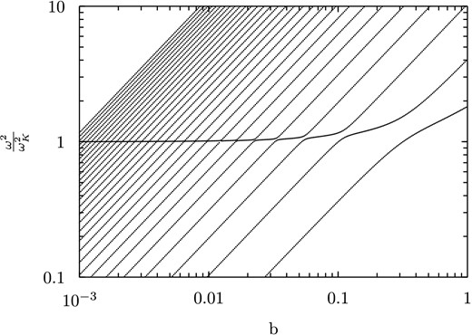
$Plot showing how the l = 2 mode frequencies of an incompressible elastic star vary with the ratio of strain to gravitational energy b. On the y-axis, frequencies are scaled by the fundamental l = 2 Kelvin mode of an incompressible fluid star, ωK. For typical neutron star parameters, ωK ∼ 2000 Hz. For a given value of b, the lowest-order modes have a similar character to those of an elastic solid, scaling as $\sim \sqrt{\frac{\mu }{\rho }}$. There is one mode around $\frac{\omega }{\omega _{\rm K}}=1$ with a hybrid fluid-elastic character, and then the higher modes again have an elastic character.$

Figure 2.

Plot showing how the l = 2 mode frequencies of an incompressible elastic star vary with the ratio of strain to gravitational energy b. On the y-axis, frequencies are scaled by the fundamental l = 2 Kelvin mode of an incompressible fluid star, ω_K. For typical neutron star parameters, ω_K ∼ 2000 Hz. For a given value of b, the lowest-order modes have a similar character to those of an elastic solid, scaling as |$\sim \sqrt{\frac{\mu }{\rho }}$|⁠. There is one mode around |$\frac{\omega }{\omega _{\rm K}}=1$| with a hybrid fluid-elastic character, and then the higher modes again have an elastic character.

Open in new tab Download slide

Next, we can use these eigenvalues to calculate the corresponding toroidal and spheroidal eigenfunctions. Fig. 3(c) shows a plot of the first 10 toroidal eigenfunctions for b = 0.01. The lowest, n = 1 eigenfunction has no nodes; each eigenfunction gains one more node with increasing n.

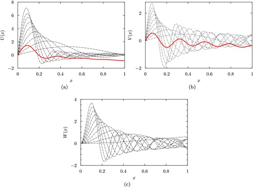
$Figure showing the U, V and W radial parts of the first ten l = 2 spheroidal and toroidal eigenfunctions for the case b = 0.01, as a function of the fractional radius $x=\frac{r}{R}$. (a) Plot of the U radial part of the first 10 spheroidal eigenfunctions. The hybrid fluid-like mode is marked in solid red; the other eigenfunctions (dashed lines) have an elastic character. (b) Plot of the V radial part of the first 10 spheroidal eigenfunctions, with the hybrid fluid-like mode marked in solid red. (c) Plot of the W radial part of the first 10 toroidal eigenfunctions.$

Figure 3.

Figure showing the U, V and W radial parts of the first ten l = 2 spheroidal and toroidal eigenfunctions for the case b = 0.01, as a function of the fractional radius |$x=\frac{r}{R}$|⁠. (a) Plot of the U radial part of the first 10 spheroidal eigenfunctions. The hybrid fluid-like mode is marked in solid red; the other eigenfunctions (dashed lines) have an elastic character. (b) Plot of the V radial part of the first 10 spheroidal eigenfunctions, with the hybrid fluid-like mode marked in solid red. (c) Plot of the W radial part of the first 10 toroidal eigenfunctions.

Open in new tab Download slide

The spheroidal eigenfunctions display more complicated behaviour. As an example, Figs 3(a) and (b) show the U and V parts of the first 10 eigenfunctions for b = 0.01. The majority of the eigenfunctions, shown as grey dashed lines, are of elastic type. These form an ordered sequence with the lowest n = 1 mode having one stationary point, the n = 2 mode having two, etc. These modes also have a very small amplitude at the surface.

The eighth eigenfunction, marked as a solid red line, has a frequency just above ω_K and exhibits very different behaviour to the rest of the set. In particular, it has a much larger amplitude at the surface. This is consistent with this eigenfunction having a hybrid fluid-elastic character: the overall shape of the eigenfunction is similar to the linear l = 2 Kelvin mode eigenfunction for a completely fluid star (equation 94), while the elastic character of the mode is evident in the oscillations superimposed on this.

This behaviour is generic for all values of b in the range b = 10⁻⁶–1 that we have studied. As b gets smaller, the gap between mode frequencies gets smaller, so that the single hybrid mode is pushed to higher n. By b = 10⁻⁶, the hybrid mode is at n = 877. For lower values of b, where the star is closer to a fluid star, we should expect the hybrid eigenfunction to approach that for a fluid star. This is indeed what we see in Fig. 4, where the hybrid mode is plotted for four different values of b. In the l = 2 case, the fluid Kelvin mode eigenfunction (equation 94) has a linear U component; the hybrid modes approach this form as b becomes smaller.

Plot showing the U radial part of the l = 2 hybrid fluid-like mode for b varying from 10−1 to 10−4. As b is made smaller, the form of the eigenfunction becomes closer to the linear eigenfunction of an incompressible fluid star.

Figure 4.

Plot showing the U radial part of the l = 2 hybrid fluid-like mode for b varying from 10⁻¹ to 10⁻⁴. As b is made smaller, the form of the eigenfunction becomes closer to the linear eigenfunction of an incompressible fluid star.

Open in new tab Download slide

Another way to obtain some insight into the behaviour of the eigenfunctions is to pick a value of n and track the variation of the eigenfunction with b. As an example, Fig. 5 is a surface plot for n = 3, showing how the U part eigenfunction changes between b = 10⁻³ and 1. We can see that the eigenfunction changes continuously, but goes through three distinct phases. For the smallest values of b on the right, the three lowest eigenfunctions are all elastic-type eigenfunctions, and so the n = 3 eigenfunction is the third elastic eigenfunction with three stationary points. As b gets larger there is a transitional area where the third mode has a hybrid character. For values of b larger than around 0.1, the hybrid mode is found at n = 1 or 2, and so the n = 3 eigenfunction is again an elastic-type function, this time the second such function with two stationary points. The contours projected on to the base of the graph show how the zeroes of the eigenfunction vary with b. This makes it clear that the intermediate, hybrid eigenfunction has a very different character, with no zeroes.

Figure 5.

Surface plot showing how the U radial part of the n = 3 eigenfunction varies with b. The eigenfunction goes through three distinct phases: in the middle region around b = 0.1 there is a transitional area where this mode has a hybrid fluid-elastic character. The contours projected on to the base of the graph show the zeroes of the eigenfunction; there are none for the hybrid mode.

Open in new tab Download slide

5.2 Rotating star

To model mode excitation of a glitching star, we will also need to account for the fact that the star is rotating. In this section, we will add the effects of rotation in to our computation of the oscillation modes of our model.

We will assume that the star is rotating slowly, in the sense that the centrifugal force is small compared to the gravitational force at the surface of the star; this is a reasonable assumption for most pulsars. This approach was used for fluid stars by Cowling & Newing (1949), and has also been developed in the geophysics literature (Backus & Gilbert 1961; MacDonald & Ness 1961; Pekeris, Alterman & Jarosch 1961). Here, we will mainly use the method of Strohmayer (1991). However, we will use somewhat different notation in our paper, based on that of Friedman & Schutz (1978), so it will be helpful to restate some of the main results in this notation.

We first write the mode equation for the spherical star (equation 80) schematically as

\begin{equation} -\omega ^2 A\boldsymbol {\xi }+ C\boldsymbol {\xi }= 0. \end{equation}

(97)

In a rotating frame this becomes

\begin{equation} -\omega ^2A \boldsymbol {\xi }+ i\omega B\boldsymbol {\xi }+ C\boldsymbol {\xi }= 0, \end{equation}

(98)

where the new operator B is defined by

\begin{equation} B\boldsymbol {\xi }\equiv 2\rho \,\boldsymbol {\Omega }\times \frac{\mathrm{d} \boldsymbol {\xi }}{\mathrm{d} t}. \end{equation}

(99)

We next make the slow rotation approximation, defining the small dimensionless quantity

\begin{equation} \varepsilon = \frac{\Omega }{\omega _*} \ll 1, \end{equation}

(100)

where |$\omega _* = \sqrt{\frac{GM}{R^3}}$|⁠. In terms of our small rotational parameter t (equation 67), we have

\begin{equation} \varepsilon = \sqrt{\frac{10}{3}}\sqrt{t}. \end{equation}

(101)

We linearize in this small parameter ε, writing

\begin{eqnarray} \boldsymbol {\xi }^\alpha = \boldsymbol {\xi }^\alpha _{(0)} + \varepsilon \boldsymbol {\xi }^\alpha _{(1)}, \end{eqnarray}

(102)

\begin{eqnarray} \omega ^\alpha = \omega ^\alpha _{(0)} + \varepsilon \omega ^\alpha _{(1)}, \end{eqnarray}

(103)

where |$\xi ^\alpha _{(0)}$| and |$\omega ^\alpha _{(0)}$| are the eigenfunctions and corresponding eigenvalues of the non-rotating star, found in the previous section. We then look for normal mode solutions of the form |$\boldsymbol {\xi }^\alpha (x,t) = {\rm e}^{{\rm i}\omega t}\boldsymbol {\xi }^\alpha (x)$|⁠. At zeroth order in ε, we retain the mode equation for the spherical star, while at first order we find that

\begin{equation} -\left(\omega ^{\alpha }_{(0)}\right)^2A_{(0)}\boldsymbol {\xi }_{(1)}^\alpha - 2\omega ^{\alpha }_{(0)}\omega _{(1)}^\alpha A_{(0)}\boldsymbol {\xi }^{\alpha }_{(0)} + i\omega ^{\alpha }_{(0)}B_{(1)}\boldsymbol {\xi }^{\alpha }_{(0)} + C_{(0)}\boldsymbol {\xi }_{(1)}^\alpha = 0, \end{equation}

(104)

where

\begin{eqnarray} (A_{(0)})_{ij} \xi ^j \equiv \rho \xi ^j \end{eqnarray}

(105)

\begin{eqnarray} (B_{(0)})_{ij} \xi ^j \equiv 2\rho \, \varepsilon _{ijk} \Omega ^j \frac{\mathrm{d} \xi ^k}{\mathrm{d} t} \end{eqnarray}

(106)

\begin{eqnarray} (C_{(0)})_{ij} \xi ^j \equiv \nabla _j (\Delta \tau ) {_i^j} + \rho \nabla _i(\Delta \Phi ). \end{eqnarray}

(107)

We next write |$\boldsymbol {\xi }_{(1)}$| as a sum over the zeroth-order eigenfunctions,

\begin{equation} \boldsymbol {\xi }_{(1)}^{\alpha } = \displaystyle\sum _{\beta }\lambda _{(1)}^{\alpha \beta }\boldsymbol {\xi }_{(0)}^{\beta }. \end{equation}

(108)

Substituting this back into the first-order equation (equation 104) and making use of the zeroth-order equation, we find that

\begin{equation} -\displaystyle\sum _{\beta } \left( \left(\omega ^{\alpha }_{(0)}\right)^2 - \left(\omega ^{\beta }_{(0)}\right)^2 \right) \lambda _{(1)}^{\alpha \beta }A_{(0)}\boldsymbol {\xi }_{(0)}^{\beta } - 2\omega ^{\alpha }_{(0)}\omega _{(1)}^{\alpha }A_{(0)}\boldsymbol {\xi }^{\alpha }_{(0)} + i\omega ^{\alpha }_{(0)}B_{(1)}\boldsymbol {\xi }^{\alpha }_{(0)} = 0. \end{equation}

(109)

This equation can then be used to find expressions for the first-order rotational corrections to the eigenfunctions and eigenvalues. To do this, we define the inner product

\begin{equation} \left\langle \boldsymbol {\eta }, \boldsymbol {\xi }\right\rangle \equiv \int _V \boldsymbol {\eta }^*\cdot \boldsymbol {\xi }\, \mathrm{d}V. \end{equation}

(110)

We show in Appendix B that the zeroth-order eigenfunctions are orthogonal with respect to the operator A₍₀₎, We will also scale the eigenfunctions so that they are orthonormal:

\begin{equation} \left\langle \boldsymbol {\xi }_{(0)}^{\alpha }, A_{(0)}\boldsymbol {\xi }_{(0)}^{\beta }\right\rangle = \delta ^{\alpha \beta }. \end{equation}

(111)

Taking the inner product of equation (109) and |$\xi _{(0)}^\alpha$| and using this orthogonality condition, we find an expression for the rotational corrections to the eigenvalues,

\begin{equation} \omega _{(1)}^{\alpha }= \frac{i}{2}\left\langle \xi _{(0)}^{\alpha },B_{(1)}\xi ^{\alpha }_{(0)}\right\rangle . \end{equation}

(112)

Similarly, to find the corrections to the eigenfunctions we can take an inner product of equation (109) and |$\xi _{(0)}^\gamma$|⁠, γ ≠ α, finding that

\begin{equation} \lambda _{(1)}^{\alpha \gamma } = \frac{i\omega ^{\alpha }_{(0)}}{ \left(\omega ^{\alpha }_{(0)}\right)^2 - \left(\omega ^{\gamma }_{(0)}\right)^2} \left\langle \xi _{(0)}^{\gamma }, B_{(1)}\xi ^{\alpha }_{(0)}\right\rangle . \end{equation}

(113)

Finally, it can be shown that for α = γ, the coefficient |$\lambda _{(1)}^{\alpha \alpha }$| can be chosen to be zero (see, for example, Rae 2002).

To calculate explicit formulae for the corrections |$\boldsymbol {\xi }_{(0)}^\alpha$| and |$\omega _{(0)}^\alpha$|⁠, it will be necessary to separate out spheroidal and toroidal corrections. The zeroth-order spheroidal and toroidal eigenfunctions |$\boldsymbol {S}_{(0)}$| and |$\boldsymbol {T}_{(0)}$| have the forms (85) and (90), respectively. Formulae for the full corrected eigenfunctions are given in Strohmayer (1991). In the m = 0 case, the eigenvalue corrections |$(\omega _{(1)} )_{\rm S}^\alpha$| and |$(\omega _{(1)})_{\rm T}^\alpha$| are zero, and the corrected eigenfunctions have the form

\begin{equation} {\boldsymbol {S}}^{nl} = {\boldsymbol {S}}_{(0)}^{nl} + \varepsilon \displaystyle\sum _{n=1}^{\infty }\left[ [ST]_{(1)}^{nl,n^{\prime }l-1}{\boldsymbol {T}}_{n^{\prime }l-1} + [ST]_{(1)}^{nl,n^{\prime }l+1}{\boldsymbol {T}}_{n^{\prime }l+1} \right], \end{equation}

(114)

\begin{equation} \boldsymbol {T}^{nl} = \boldsymbol {T}_{(0)}^{nl} + \varepsilon \displaystyle\sum _{n^{\prime }=1}^{\infty }\left[ [TS]_{(1)}^{nl,n^{\prime }l-1}\boldsymbol {S}_{(0)}^{n^{\prime }l-1} + [TS]_{(1)}^{nl,n^{\prime }l+1}\boldsymbol {S}_{(0)}^{n^{\prime }l+1} \right], \end{equation}

(115)

where the [ST]₍₁₎ are the coefficients of the toroidal corrections to the spheroidal eigenfunctions and the [TS]₍₁₎ are the coefficients of the spheroidal corrections to the toroidal eigenfunctions.

To calculate these corrections numerically, we again scale our equations so that the star has unit radius R = 1, and that the l = 2 fluid Kelvin mode has ω_K = 1. With this choice, the parameter σ_* (equation 100) becomes |$\sigma _* = \frac{\sqrt{5}}{2}$|⁠.

The analytic expressions for the corrected eigenfunctions (114) and (115) include an infinite sum over the radial eigenvalue number n. For numerical work we will need to truncate these eigenfunctions, calculating the sum only up to some maximum value N. We will label these truncated eigenfunctions as |$\boldsymbol {S}^\alpha _N$| and |$\boldsymbol {T}^\alpha _N$|⁠.

The value of N we choose to cut off at will depend on b. It will turn out that in the special case where the angular velocity of the star after the glitch is zero, the majority of the energy released in the glitch goes into the hybrid fluid-elastic mode. This effect becomes more pronounced as b becomes smaller. As rotation is only a small correction, this will largely hold true even in the rotating case. This means that the cut-off N should be chosen to be somewhat larger than the n number of the hybrid mode. We will investigate the cases b = 10⁻¹, 10⁻², 10⁻³. In these cases the hybrid mode is at n = 2, 7 and 27 respectively. We will choose our cut-offs for each of these cases to be at N = 10, 15 and 40. To check that we have truncated at a high-enough value N, we have checked that the partial sums |$\boldsymbol {S}^\alpha _N$| and |$\boldsymbol {T}^\alpha _N$| converge. As an example, we show this here for the spheroidal l = 2, n = 1 eigenfunction, with b = 10⁻¹, by plotting the function

\begin{equation} \left(\boldsymbol {S}^{{\rm converge}}\right)^{120}_n(x) \equiv \left|\frac{\boldsymbol {S}^{120}_n(x) - \boldsymbol {S}^{120}_{10}(x)}{\boldsymbol {S}^{120}_{10}(x)}\right| \end{equation}

(116)

for k = 1, …, 10. For the spheroidal corrections, only the ϕ component of |$(\boldsymbol {S}^{{\rm converge}})^{120}_n(x)$| is non-zero. This component is plotted in Fig. 6, with |$(\boldsymbol {S}^{{\rm converge}})^{120}_1(x)$| in black and |$(\boldsymbol {S}^{{\rm converge}})^{120}_{10}(x)$| in green, showing convergence as more modes are added to the sum.

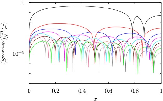
$Figure showing the convergence of the rotational corrections to the spheroidal l = 2, n = 1 eigenfunctions for b = 10−1, as the corrections are truncated at progressively higher values of the radial eigenvalue N. In particular, the ϕ component of the functions $(S^{{\rm converge}})^{n20}_N$ (equation 116) is plotted for N = 1 (plotted in black) up to N = 9 (plotted in green).$

Figure 6.

Figure showing the convergence of the rotational corrections to the spheroidal l = 2, n = 1 eigenfunctions for b = 10⁻¹, as the corrections are truncated at progressively higher values of the radial eigenvalue N. In particular, the ϕ component of the functions |$(S^{{\rm converge}})^{n20}_N$| (equation 116) is plotted for N = 1 (plotted in black) up to N = 9 (plotted in green).

Open in new tab Download slide

6 PROJECTING THE INITIAL DATA

We are now in a position to project our initial data for the displacement and velocity fields against the eigenfunctions of Star D (equations 114 and 115) after the glitch. This initial data has the form

\begin{eqnarray} \boldsymbol {\xi }^{{\rm DC}} = \left(\frac{5z}{R^2} \left(3r^3-8R^2r\right)\right)P_2\,\hat{\boldsymbol {r}} + \left(\frac{5z}{R^2} \left(\frac{5}{2} r^4-4R^2r^2\right)\right){\nabla }P_2, \end{eqnarray}

(117)

\begin{eqnarray} \dot{\boldsymbol {\xi }}^{{\rm DC}} = -\sqrt{\frac{3}{8}}\,\sqrt{t}\,z r \left(\hat{\boldsymbol {r}}\times {\nabla }P_1\right), \end{eqnarray}

(118)

where we have rewritten the velocity initial data (equation 52) to show that it has a pure toroidal form (equation 90). We can in fact think of the velocity data as a zero-frequency l = 1 toroidal eigenfunction. There are two free parameters in the initial data: z (equation 20), related to the size of the glitch, and t (equation 67), related to the angular velocity of Star B. As z just produces an overall scaling of the initial data, we shall set z = 1 in the following numerical work, and only investigate the change in amplitudes produced as we vary t and b. As in Section 5, we will also scale the initial data so that the radius of the star R = 1, and the l = 2 fluid Kelvin mode ω_K = 1.

Before considering the full problem, we can get some useful insight from the special case where the star spins down to zero angular velocity (Ω_B = 0) before the ‘glitch’, modelled as a sudden loss of strain from the star. Although this is not a realistic model – we have lost the key observational feature of the glitch, the change in rotation rate of the star – there are good reasons to discuss this first. For a start, it is easier to interpret the results for this simpler case, and certain features of these will carry over to the more realistic case where the star is still rotating before the glitch. We can also check that the results for the rotating problem converge to the non-rotating one as rotation becomes small.

Another reason for considering the non-rotating problem first is that the rotation of the star introduces significant complications to the projection scheme. One of these is that the eigenfunctions of the rotating star are no longer orthogonal. Another is the existence of the zero eigenvalue l = 1 toroidal mode (equation 118) that our velocity initial data is built from. As this mode is zero frequency, it will not have the e^iωt time-dependence of the other eigenfunctions and we will have to consider it separately. We will discuss these problems in Section 6.2.

6.1 Special case: glitch at zero spin

For the special case where Ω_B = 0, the velocity field part of the initial data (equation 118) is zero. For the displacement field, although there is no change in angular velocity of the star at the glitch, we still have a finite value of the parameter z (equation 20),

\begin{equation} z\vert _{\Omega _{\rm B} = 0} = \frac{5}{2\pi G\rho }\, b \Omega _{\rm A}^2, \end{equation}

(119)

and the displacement field initial data takes the same form (equation 117) as for the general, rotating case. Our only free parameter in this Ω_B = 0 case is z, which we have set to unity.

The eigenfunctions we are projecting against are those of the non-rotating star (equations 87 and 88) with time-dependence

\begin{equation} \boldsymbol {\xi }_{(0)}^\alpha (x,t) \equiv \boldsymbol {\xi }^\alpha _{(0)}(x){\rm e}^{{\rm i}\omega ^\alpha t}. \end{equation}

(120)

The initial data is then a sum over these modes, with each eigenfunction |$\boldsymbol {\xi }^\alpha$| excited by some amplitude b^α. The initial data is real, so to ensure that the sum over the eigenfunctions is also real we write it as

\begin{eqnarray} \boldsymbol {\xi }^{{\rm ID}}(x) = \frac{1}{2}\sum _\alpha \left[ b^\alpha \boldsymbol {\xi }^\alpha _{(0)} (x) + b^{*\alpha } \boldsymbol {\xi }^{*\alpha }_{(0)}(x) \right], \end{eqnarray}

(121)

\begin{eqnarray} \dot{\boldsymbol {\xi }}^{{\rm ID}}(x) = \frac{1}{2}\displaystyle\sum _\alpha \left[ i\omega ^\alpha b^\alpha \boldsymbol {\xi }^\alpha _{(0)} (x) -i\omega ^\alpha b^{*\alpha } \boldsymbol {\xi }^{*\alpha }_{(0)} (x) \right]. \end{eqnarray}

(122)

The complex conjugate is not really necessary at the moment, where we are projecting against the real eigenfunctions of a non-rotating star. However, it will be required later when we extend to the rotating case and the eigenfunctions have an imaginary part, so for consistency we keep it in here. We will scale our eigenfunctions so that they are orthonormal with respect to the inner product (equation 110) defined in Section 5:

\begin{equation} \left\langle \boldsymbol {\xi }^\beta _{{\rm (0)}}, \boldsymbol {\xi }^\alpha _{{\rm (0)}} \right\rangle = \delta ^{\alpha \beta }. \end{equation}

(123)

By taking the inner products of |$\boldsymbol {\xi }^{{\rm ID}}$| and |$\dot{\boldsymbol {\xi }}^{{\rm ID}}$| with an eigenfunction |$\boldsymbol {\xi }^\alpha$|⁠, we find that the amplitudes b^α satisfy

\begin{equation} b^\alpha = -\frac{i}{\omega ^\alpha }\left( \left\langle \boldsymbol {\xi }^\alpha _{{\rm (0)}},\dot{\boldsymbol {\xi }}^{{\rm ID}}\right\rangle +i\omega ^\alpha \left\langle \boldsymbol {\xi }^\alpha _{{\rm (0)}},\boldsymbol {\xi }^{{\rm ID}}\right\rangle \right). \end{equation}

(124)

Fig. 7 shows the results of the projection for different values of b, ranging from the high value of b = 0.1 (Fig. 7a) down to the physical range of b = 10⁻⁵ (Fig. 7e) and b = 10⁻⁶ (Fig. 7f). The x-axis shows the radial number of the mode, while the y-axis shows the amplitude of that mode. In all of these plots, the hybrid fluid-elastic mode discussed in Section 5 has the greatest amplitude; this is the mode with the frequency closest to the fundamental Kelvin mode of a purely fluid star. For the higher values of b, the lowest-order modes are also excited to significant amplitudes: these are the shear modes with the lowest number of radial nodes. However, for physical values of b (b ∼ 10⁻⁵), only the fluid-elastic mode is appreciably excited. Finally, as a check we can also show that we are reproducing the initial data correctly by reconstructing the sum over the eigenfunctions (equation 120) with our calculated amplitudes b^α. The results of this are shown in Appendix A.

Figure 7.

Figure showing the results of the projection for different values of b. For clarity, individual vertical bars are not displayed for plots (c)–(f). The x-axis shows the radial number of the mode, while the y-axis shows the amplitude of that mode. The hybrid fluid-elastic mode has the largest amplitude; this becomes more pronounced as b is made smaller.

Open in new tab Download slide

6.2 The general case: glitch at arbitrary spin

We will now move on to the projection of the initial data in the general case, where Star B is rotating before the glitch. Here, we will have to deal with the zero eigenvalue l = 1 toroidal mode (equation 118) that our velocity initial data is built from. As this mode is zero frequency, it will not have the e^iωt time-dependence of the other modes and we will have to consider it separately. For the purposes of this section, we will label the zero-frequency eigenfunction |$\boldsymbol {\xi }_{(0)}^1$|⁠, with eigenvalue |$\omega _{(0)}^1$|⁠. To find the time-dependence of |$\boldsymbol {\xi }_{(0)}^1(x,t)$|⁠, we go back to the governing equation for the zeroth-order eigenfunctions,

\begin{equation} A_{(0)}\frac{\mathrm{\partial} ^2 \boldsymbol {\xi }^\alpha _{(0)}}{\mathrm{\partial} {t}^2} + C_{(0)}\boldsymbol {\xi }^\alpha _{(0)} = 0. \end{equation}

(125)

In the case of our zero frequency mode, the eigenfunction describes rigid rotation, so that its velocity field is constant in time,

\begin{equation} \frac{\mathrm{\partial} ^2 \boldsymbol {\xi }^1_{(0)}}{\mathrm{\partial} {t}^2} = 0. \end{equation}

(126)

The solutions of this are |$\boldsymbol {\xi }^1_{(0)}(x,t) = \boldsymbol {\xi }^1_{(0)}(x)T(t)$| with

\begin{equation} T(t) = C^1t + D^1, \end{equation}

(127)

C¹ and D¹ real. The governing equation for the zeroth-order modes (equation 125) becomes just

\begin{equation} C_{(0)} \boldsymbol {\xi }^1_{(0)} = 0. \end{equation}

(128)

We can also look at the first-order corrections |$\boldsymbol {\xi }^1_{(1)}=\displaystyle\sum _\beta \lambda _{(1)}^{1\beta }\boldsymbol {\xi }_{(0)}^\beta$| to this mode. These satisfy the equation

\begin{equation} C_{(0)} \boldsymbol {\xi }^1_{(1)} = 0, \end{equation}

(129)

which has the same form as the equation for the zeroth-order modes. This means that we can absorb them into the zeroth-order mode |$\boldsymbol {\xi }^0_{(1)}$|⁠, so that the corrections |$\lambda _{(1)}^{1\beta } =0$|⁠. We will now describe a scheme to allow us to project the initial data against the eigenfunctions |$\boldsymbol {\xi }$| of the rotating star, which are not orthogonal, by using the orthogonality of the zeroth-order eigenfunctions |$\boldsymbol {\xi }_{(0)}$|⁠. We start by writing out the time-dependence explicitly for the displacement field |$\boldsymbol {\xi }(x,t)$|⁠:

\begin{equation} \boldsymbol {\xi }(x,t) = \left[ Ct + D\right]\boldsymbol {\xi }_{(0)}^1(x) + \frac{1}{2}\displaystyle\sum _{\alpha =2}^\infty \left[ b^\alpha \boldsymbol {\xi }^\alpha (x){\rm e}^{{\rm i}\omega ^\alpha t} + b^{*\alpha }\boldsymbol {\xi }^{*\alpha } (x){\rm e}^{-{\rm i}\omega ^\alpha t} \right]. \end{equation}

(130)

Here, we have separated out the zero eigenvalue mode – note that we can just use its zeroth-order form because it has no first-order corrections. To make sure that the data for the other modes is real we have added on the complex conjugate. The complex coefficients b^α contain the amplitude and phase of each mode. It will be convenient to write the zero frequency eigenfunction |$\boldsymbol {\xi }_{(0)}^1$| in a similar way to the other eigenfunctions by defining

\begin{eqnarray} C^1 = \frac{i}{2}(b^1 - (b^1)^*), \end{eqnarray}

(131)

\begin{eqnarray} D^1 = \frac{1}{2}(b^1 + (b^1)^*), \end{eqnarray}

(132)

where b¹ is a complex constant, so that equation (130) becomes

\begin{equation} \boldsymbol {\xi }(x,t) = \left[ \frac{i}{2}(b^1 - (b^1)^*)t +\frac{1}{2}( b^1 + (b^1)^*)\right]\boldsymbol {\xi }_{(0)}^1(x) + \frac{1}{2}\displaystyle\sum _{\alpha =2}^\infty \left[ b^\alpha \boldsymbol {\xi }^\alpha (x){\rm e}^{{\rm i}\omega ^\alpha t} + b^{*\alpha }\boldsymbol {\xi }^{*\alpha } (x){\rm e}^{-{\rm i}\omega ^\alpha t} \right]. \end{equation}

(133)

Differentiating this, the velocity field is

\begin{equation} \dot{\boldsymbol {\xi }}(x,t) = \frac{i}{2}( b^1 - (b^1)^*)\boldsymbol {\xi }_{(0)}^1(x) + \frac{1}{2}\displaystyle\sum _{\alpha =2}^\infty \left[ i\omega _{(0)}^\alpha b^\alpha \boldsymbol {\xi }^\alpha (x,t) -i\omega _{(0)}^\alpha b^{*\alpha } \boldsymbol {\xi }^{*\alpha } (x,t) \right], \end{equation}

(134)

where we have used the fact that there are no rotational corrections to the zeroth-order eigenvalues ω₍₀₎ in the m = 0 case we are interested in. We can combine |$\boldsymbol {\xi }_{(0)}^1$| with the other eigenfunctions by making the definition

\begin{equation} \tilde{\omega }_{(0)}^\alpha = \left\lbrace \begin{array}{@{}l@{\quad }l@{}}1 & \alpha = 1, \\ \omega _{(0)}^\alpha & {\rm otherwise}. \end{array}\right. \end{equation}

(135)

Specializing to t = 0, we can then use this along with our definitions of C (equation 131) and D (equation 132) to write the initial data in the neat form

\begin{eqnarray} \boldsymbol {\xi }^{{\rm ID}}(x) \equiv \boldsymbol {\xi }(x,0) = \frac{1}{2}\displaystyle\sum _{\alpha = 1}^\infty \left[ b^\alpha \boldsymbol {\xi }^\alpha (x) + {\rm c.c.} \right], \end{eqnarray}

(136)

\begin{eqnarray} \dot{\boldsymbol {\xi }}^{{\rm ID}}(x)\equiv \dot{\boldsymbol {\xi }}(x,0) = \frac{1}{2}\displaystyle\sum _{\alpha = 1}^\infty \left[ i\tilde{\omega }_{(0)}^\alpha b^\alpha \boldsymbol {\xi }^\alpha (x) + {\rm c.c.} \right]. \end{eqnarray}

(137)

Next, we expand the eigenfunctions in the sum to first order in rotation (102). Introducing the notation

\begin{equation} \boldsymbol {\xi }^\alpha = \displaystyle\sum _{\beta =1}^\infty \left(\delta ^{\alpha \beta } + \lambda _{(1)}^{\alpha \beta }\right) \boldsymbol {\xi }^\beta _{{\rm (0)}} \equiv \displaystyle\sum _{\beta =1}^\infty \Lambda ^{\alpha \beta } \boldsymbol {\xi }^\beta _{{\rm (0)}}, \end{equation}

(138)

we then have

\begin{eqnarray} \boldsymbol {\xi }^{{\rm ID}} (x) &= \displaystyle\sum _{\alpha =1}^{\infty }\left[ \frac{b^{\alpha }}{2} \left( \displaystyle\sum _{\beta =1}^{\infty }\Lambda ^{\alpha \beta }\boldsymbol {\xi }_{(0)}^\beta \right) + \frac{(b^{\alpha })^*}{2} \left( \displaystyle\sum _{\beta =1}^{\infty }(\Lambda ^*)^{\alpha \beta } \boldsymbol {\xi }_{(0)}^\beta \right) \right], \end{eqnarray}

(139)

\begin{eqnarray} \dot{\boldsymbol {\xi }}^{{\rm ID}} (x) &= \displaystyle\sum _{\alpha =1}^{\infty } \left[ i\tilde{\omega }^\alpha \frac{b^{\alpha }}{2} \left( \displaystyle\sum _{\beta =1}^{\infty }\Lambda ^{\alpha \beta }\boldsymbol {\xi }_{(0)}^\beta \right) -i\tilde{\omega }^\alpha \frac{(b^{\alpha })^*}{2} \left( \displaystyle\sum _{\beta =1}^{\infty }(\Lambda ^*)^{\alpha \beta } \boldsymbol {\xi }_{(0)}^\beta \right) \right], \end{eqnarray}

(140)

where the corrections to |$\boldsymbol {\xi }_{(0)}^1$| are λ^1β = 0. We can take an inner product with another zeroth-order eigenfunction |$\boldsymbol {\xi }_{(0)}^\gamma$| to obtain

\begin{eqnarray} \left\langle \boldsymbol {\xi }_{(0)}^\gamma ,\boldsymbol {\xi }^{{\rm ID}} (x) \right\rangle &= \displaystyle\sum _{\alpha =1}^{\infty }\left[ \frac{b^{\alpha }}{2} \left( \Lambda ^{\alpha \gamma } \right) + \frac{(b^{\alpha })^*}{2} \left( (\Lambda ^*)^{\alpha \gamma } \right) \right], \end{eqnarray}

(141)

\begin{eqnarray} \left\langle \boldsymbol {\xi }_{(0)}^\gamma ,\dot{\boldsymbol {\xi }}^{{\rm ID}} (x)\right\rangle &= \displaystyle\sum _{\alpha =1}^{\infty } \left[ i\tilde{\omega }^\alpha \frac{b^{\alpha }}{2} \left( \Lambda ^{\alpha \gamma } \right) -i\tilde{\omega }^\alpha \frac{(b^{\alpha })^*}{2} \left( (\Lambda ^*)^{\alpha \gamma } \right) \right]. \end{eqnarray}

(142)

In practice, when carrying out a projection numerically we will only consider a finite sum, cutting off at some sufficiently large β = N. We can then view equations (141) and (142) as vectors of N equations, so that we can rewrite them as

\begin{eqnarray} \boldsymbol {x} = \frac{1}{2}(\Lambda ^{\rm T} \boldsymbol {b} + (\Lambda ^{\rm T})^*\boldsymbol {b}^*), \end{eqnarray}

(143)

\begin{eqnarray} \dot{\boldsymbol {x}} = \frac{1}{2}(\Omega ^{\rm T} \boldsymbol {b} + (\Omega ^{\rm T})^*\boldsymbol {b}^*), \end{eqnarray}

(144)

where the vectors |$\boldsymbol {x}$| and |$\dot{\boldsymbol {x}}$| are defined by

\begin{eqnarray} x^\beta \equiv \left\langle \boldsymbol {\xi }^\beta ,\boldsymbol {\xi }^{{\rm ID}}(x)\right\rangle \end{eqnarray}

(145)

\begin{eqnarray} \dot{x}^\beta \equiv \left\langle \boldsymbol {\xi }^\beta ,\dot{\boldsymbol {\xi }}^{{\rm ID}}(x)\right\rangle , \end{eqnarray}

(146)

for β = 1, …, N, and the matrix Ω is built from Λ (equation 138) as

\begin{eqnarray} \Omega \equiv D\Lambda , \end{eqnarray}

(147)

\begin{eqnarray} D\equiv {\rm diag}\,[i\tilde{\omega }^1, i\tilde{\omega }^2,\dots , i\tilde{\omega }^N]. \end{eqnarray}

(148)

Solving for |$\boldsymbol {b}$|⁠, we have

\begin{equation} \boldsymbol {b} = 2{\rm A}^{-1}\left\lbrace \left[(\Lambda ^*)^{{\rm T}}\right]^{-1}\boldsymbol {x} -\left[(\Omega ^*)^{{\rm T}}\right]^{-1}\dot{\boldsymbol {x}} \right\rbrace \end{equation}

(149)

where A is the matrix

\begin{equation} {\rm A}=\left[(\Lambda ^*)^{{\rm T}}\right]^{-1}\Lambda ^{{\rm T}} -\left[(\Omega ^*)^{{\rm T}}\right]^{-1}\Omega ^{{\rm T}}. \end{equation}

(150)

These coefficients |$\boldsymbol {b}$| can then be used to reconstruct the initial data, as

\begin{eqnarray} \boldsymbol {\xi }^{{\rm reconstruct}}(N) = \frac{1}{2}\displaystyle\sum _{\alpha =1}^N\left[ b^\alpha \Lambda ^{\alpha \beta } \boldsymbol {\xi }_{(0)}^\beta + (b^*)^\alpha \left(\Lambda ^*\right)^{\alpha \beta }\boldsymbol {\xi }_{(0)}^\beta \right], \end{eqnarray}

(151)

\begin{eqnarray} \dot{\boldsymbol {\xi }}^{{\rm reconstruct}}(N) = \frac{1}{2}\displaystyle\sum _{\alpha =1}^N\left[ i\omega ^\alpha b^\alpha \Lambda ^{\alpha \beta } \boldsymbol {\xi }_{(0)}^\beta - i\omega ^\alpha (b^*)^\alpha \left(\Lambda ^*\right)^{\alpha \beta }\boldsymbol {\xi }_{(0)}^\beta \right]. \end{eqnarray}

(152)

To make use of this projection scheme, we first need to construct the matrix Λ. To do this, we will need to decide which modes α = (n, l, m) we are keeping in the projection, and choose an ordering for the mode indices α. Looking at the initial data we are projecting, we can see that the displacement field (117) is spheroidal l = 2 and m = 0. From the form of the full, corrected spheroidal eigenfunctions (equation 114), this can be expected to couple to l = 1 and 3 toroidal m = 0 modes. The velocity field (118) is built from the toroidal l = 1, m = 0 zero-frequency mode, which has no first-order corrections. However, from the form of the corrected toroidal eigenfunctions (115), the l = 2 spheroidal eigenfunctions can be expected to couple to this mode. Motivated by this, we will choose to consider only m = 0 and also to cut off at l = 3, including only l = 1, 2, 3 (the l = 0 radial modes are all zero for an incompressible star). Counting both spheroidal and toroidal eigenfunctions, this gives us 6N eigenfunctions in total. This is illustrated in Fig. 8.

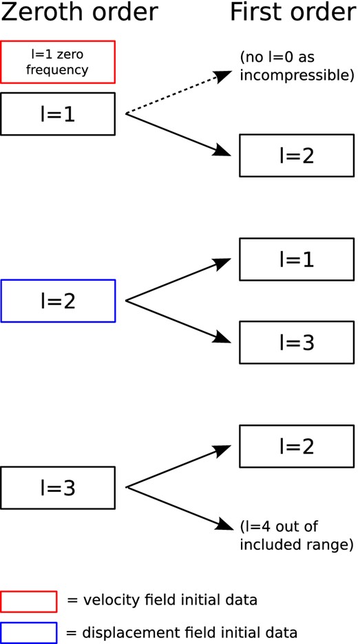
Figure 8.

Schematic showing how the zeroth-order modes couple to other modes at first order in rotation. The displacement field has an l = 2 form and couples to l = 1 and 3; this is shown in blue. The velocity field, shown in red, has the form of a zero-frequency l = 1 mode; it has no rotational corrections. The other modes in the range we are considering are also shown. The l = 1 modes only couple to l = 2, while for the l = 3 modes, only the l = 2 coupling falls into the considered range.

Open in new tab Download slide

We can then write each of the zeroth-order eigenfunctions we plan to use as one entry of a vector of length 6N, which schematically looks like

\begin{equation} \left(\begin{array}{c}{}[S1]_N \\ {}[T1]_N \\ {}[S2]_N \\ {}[T2]_N \\ {}[S3]_N \\ {}[T3]_N \\ \end{array}\right). \end{equation}

(153)

Here [S1]_N is a vector of the first N spheroidal l = 1 eigenfunctions, [T1]_N is a vector of the first N toroidal l = 1 eigenfunctions, etc. The corrected eigenfunctions are then obtained by acting on this vector with the 6N × 6N matrix Λ (equation 138), which has the form

\begin{equation} \left(\begin{array}{cccccc}I_N &\quad 0 &\quad 0 &\quad \varepsilon [ST12]_N &\quad 0 &\quad 0 \\ 0 &\quad I_N &\quad \varepsilon [TS12]_N &\quad 0 &\quad 0 &\quad 0 \\ 0 &\quad \varepsilon [ST21]_N &\quad I_N &\quad 0 &\quad 0 &\quad \varepsilon [ST23]_N \\ \varepsilon {[TS21]_N} &\quad 0 &\quad 0 &\quad I_N &\quad \varepsilon [TS23]_N &\quad 0 \\ 0 &\quad 0 &\quad 0 &\quad \varepsilon [ST32]_N &\quad I_N &\quad 0 \\ 0 &\quad 0 &\quad \varepsilon [TS32]_N &\quad 0 &\quad 0 &\quad I_N \end{array} \right). \end{equation}

(154)

Each entry represents an N × N matrix. Most off-diagonal entries are zero apart from a few blocks. For l = 2 these are the l = 1 and 3 toroidal corrections to the spheroidal eigenfunctions, [ST21]_N and [ST23]_N, and the l = 1 and 3 spheroidal corrections to the toroidal eigenfunctions, [TS21]_N and [TS23]_N. For l = 1 there are only l = 2 corrections; this is also true for l = 3 as we are not including l = 4.

6.3 Results of the projection

We carried out the projection using this numerical scheme for the cases b = 10⁻¹, 10⁻², 10⁻³. As with the calculation of the rotational corrections of the eigenfunctions, we cut off at N = 10, 15 and 40 respectively, with these values chosen so that the hybrid fluid-elastic mode is within the range for each case. The increasingly high n value of this mode for small b, and the fact that the calculation of the 6N × 6N Λ matrix is computationally intensive, meant that we did not investigate any smaller values of b.

For given b, we also need to consider what parameter range of t our scheme is valid for. We have used the slow rotation approximation to calculate the modes. Considering the form of the eigenvalue equation for the rotating star (equation 98), we can expect this to be a good approximation when ω²A is large compared to εωB, i.e when |$\frac{\Omega _{\rm B}}{\omega }\ll 1$|⁠. We have |$\Omega _{\rm B} \sim \sqrt{t}$|⁠, but we also have to take into consideration which mode ω we are looking at. The elastic modes scale with b, so that for the lowest modes with small n value we need |$\frac{\sqrt{t}}{b}\ll 1$|⁠. The hybrid fluid-like mode has a scaling |$\sqrt{G\rho }$| – we have scaled our numerical results so that this is of order unity, so for this mode we only need |$\sqrt{t}\ll 1$|⁠.

The results for b = 10⁻² are shown in detail as an illustrative example. In this case, we only have |$\frac{\sqrt{t}}{b}<10^{-1}$| for t < 10⁻⁴), so cannot expect our results to be reliable for the lowest n modes when t is larger than this. Around the n = 8 hybrid fluid-elastic mode, we can instead expect the results to be reliable when |$\sqrt{t}$| is small, i.e. from around t = 10⁻² onwards.

Fig. 9 shows the calculated amplitudes of the modes for values of log₁₀t = −1, −2, …, −6. These amplitudes are non-zero for the spheroidal l = 2 and toroidal l = 1 and 3 cases. For the spheroidal l = 2 and toroidal l = 1 cases, the first 15 modes are shown, while for the toroidal l = 3 modes the cut-off is at n = 14, because our numerical scheme does not reproduce the highest l = 3 mode correctly. To test this, we tried cutting off at lower values of N, and found that the l = 3, n = N mode is then not correct; to obtain the n = 15 mode we would have to cut off at N = 16.

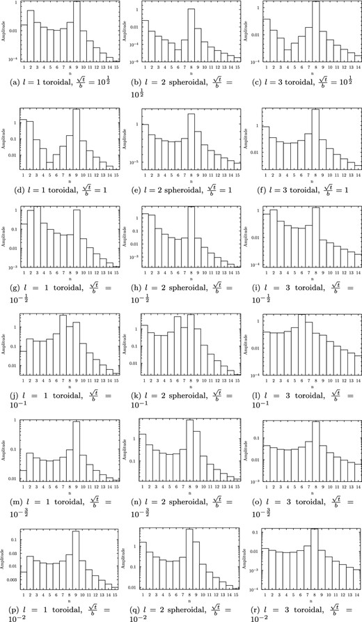
Figures showing the amplitude of each excited mode for the case b = 10−2 and log10t = −1, …, −6, where we have cut off at radial eigenvalue N = 15.

Figure 9.

Figures showing the amplitude of each excited mode for the case b = 10⁻² and log₁₀t = −1, …, −6, where we have cut off at radial eigenvalue N = 15.

Open in new tab Download slide

As a first consistency check, we can see that as t is made smaller, the results reproduce that of the non-rotating case: below t = 10⁻⁵, the l = 2 spheroidal amplitudes become very similar to those when t = 0, shown in Fig. 9(e), while the l = 1 and 3 amplitudes appear to roughly scale with |$\sqrt{t}$|⁠, as would be expected from the size of the rotational corrections (equation 101) to the first-order eigenfunctions.

For t ≥ 10⁻⁴, the modes excited vary considerably from the non-rotating case, and there is no clear pattern visible in the figure. We can obtain greater insight by instead focusing on one mode at a time, and tracking the amplitude as a continuous function of t; this is shown in Fig. 10 for the lowest n modes (n = 1, 2, 3) and also for some values of n around the hybrid mode (n = 7, 8, 9). The amplitude is plotted on the y-axis, while the x-axis shows −log₁₀t.

Figures showing how the amplitude in each mode varies with t for b = 10−2. The lowest-order modes are shown (n = 1, 2, 3), along with those around the n = 8 hybrid mode (n = 7, 8, 9). Amplitude is plotted on the y-axis, while the x-axis shows −log10t.

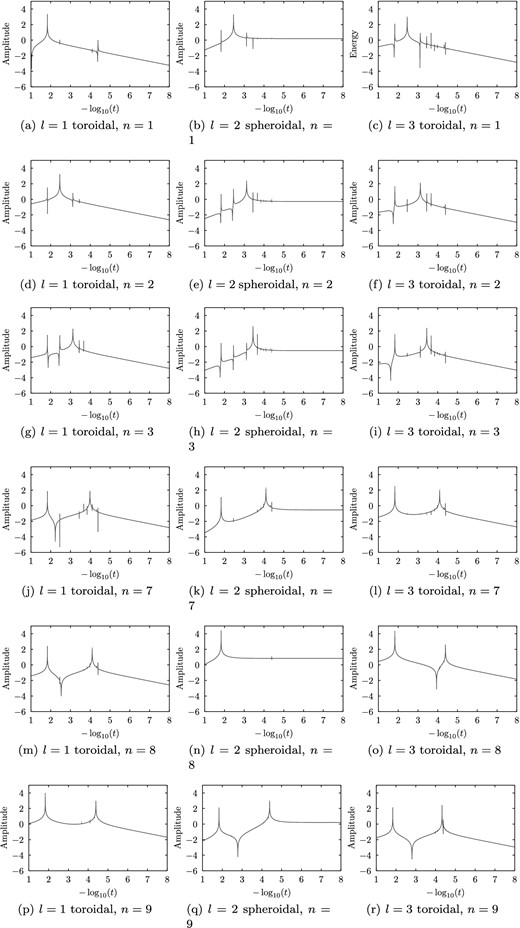
Figure 10.

Figures showing how the amplitude in each mode varies with t for b = 10⁻². The lowest-order modes are shown (n = 1, 2, 3), along with those around the n = 8 hybrid mode (n = 7, 8, 9). Amplitude is plotted on the y-axis, while the x-axis shows −log₁₀t.

Open in new tab Download slide

For the l = 2 modes, we can again see that as t is made smaller, the amplitude converges to that of the non-rotating case, while the l = 1 and 3 modes drop off with |$\sqrt{t}$| as expected. For each mode, this happens once |$\frac{\sqrt{t}}{b} \ll 1$|⁠. However, for higher values of t, there are a number of ‘spikes’ in the amplitude in each mode, small parameter ranges of t over which the amplitude changes rapidly. We currently have no clear explanation for the existence of these spikes, but have checked these are stable under the choice of cut-off N: as N is made smaller, some of the detailed features are lost, but the larger spikes remain. We also see somewhat different behaviour for the hybrid n = 8 mode, with fewer spikes in the amplitude.

A similar picture holds for b = 10⁻¹ and 10⁻³. Fig. 11 shows a few representative plots of the amplitude of the l = 2 spheroidal modes for these cases. For b = 10⁻¹, we have plotted the amplitudes of the n = 1, 2 modes and the n = 3 hybrid mode. Similarly, for b = 10⁻³ we plot n = 1 and 2, and the hybrid mode n = 27. In both cases we again see convergence to the non-rotating case once |$\frac{\sqrt{t}}{b} \ll 1$|⁠. For b = 10⁻³, as with b = 10⁻², the amplitude of the hybrid mode shows different, smoother behaviour as t is varied; this is not so apparent for b = 10⁻¹, where the hybrid mode is less distinct from the other modes of the star.

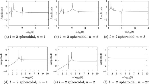
Figures showing how the amplitudes of the l = 2 spheroidal modes vary with t for b = 10−1 and 10−3. The lowest-order n = 1, 2 modes are shown in each case, along with the hybrid mode (n = 3 for b = 10−1, and n = 27 for b = 10−3). The amplitude is plotted on the y-axis, while the x-axis shows −log10t.

Figure 11.

Figures showing how the amplitudes of the l = 2 spheroidal modes vary with t for b = 10⁻¹ and 10⁻³. The lowest-order n = 1, 2 modes are shown in each case, along with the hybrid mode (n = 3 for b = 10⁻¹, and n = 27 for b = 10⁻³). The amplitude is plotted on the y-axis, while the x-axis shows −log₁₀t.

Open in new tab Download slide

A final important check is that we can use the calculated amplitudes to reconstruct the initial data. This is shown in Appendix A.

7 CONCLUSIONS

We have made order-of-magnitude estimates of the maximum energy released in a starquake, finding maximum oscillation amplitudes of |$\frac{\delta r}{R}\sim 10^{-6}$| and characteristic strains of ∼4 × 10⁻²⁴ Hz^−1/2 in the upper limit where all energy lost in the glitch is put into oscillations. For the case of a completely solid quark star, we find larger maximum amplitudes of |$\frac{\delta r}{R}\sim 10^{-2}$| can be sustained, with corresponding characteristic strains of ∼5 × 10⁻²² Hz^−1/2. In each case, these estimates are for a large change in the angular velocity of the star between glitches.

We have also developed a toy model for starquakes, in which all strain is suddenly lost from the star at the glitch. We first considered a simplified version in which the star is not rotating before the glitch, and found that the excited modes are l = 2 spheroidal oscillations. Out of these, the oscillation mode preferentially excited is a hybrid fluid-elastic mode similar to the Kelvin mode of an incompressible fluid star. The addition of rotation introduces excitation of l = 1 and 3 toroidal modes of the star. The hybrid mode is still strongly excited, but other modes of the star with an elastic character are also excited to a high level over small parameter ranges of the rotation rate; we currently have no clear explanation for this behaviour, but have tested it is stable under changing the number of radial modes we include in the set we project against.

To move from our current toy model to a more realistic model of a starquake, there are a number of extensions we need to consider. First, we would need to include the fluid core of the star in our model. This would complicate the spectrum of oscillation modes by adding extra ones connected to the fluid-elastic interface. We could also consider using a more realistic equation of state rather than our incompressible model, introducing new p- and g-modes to the mode spectrum.

It would also be necessary to improve the model for the starquake itself. At the moment, we have an acausal mechanism in which all strain is lost from the star instantaneously. In a realistic scenario, the quake would propagate across the star over time, possibly in the form of surface cracks. The new time-scale introduced here could strongly affect which modes of the star are excited. However, this time-scale is not well-constrained observationally.

The oscillations produced by a starquake would be expected to shake the magnetosphere at the surface of the star, which could lead to radio emission connected with the starquake, possibly at a level that could be resolved with the new generation of radio telescopes. It would be interesting to make some estimates of this with a toy model of how the pulsar could shake magnetic field lines in the magnetosphere.

LK acknowledges support via an STFC PhD studentship, while DIJ acknowledges support from the STFC via grant number ST/H002359/1. The authors also acknowledge partial support from ‘NewCompStar’, COST Action MP1304.

REFERENCES

Abadie

J.

et al. ,

Phys. Rev. D

,

2011

, vol.

83

pg.

042001

Crossref

Search ADS

Aizenman

M.

Smeyers

P.

Weigert

A.

,

A&A

,

1977

, vol.

58

pg.

41

Alpar

M. A.

Pines

D.

Anderson

P. W.

Shaham

J.

,

ApJ

,

1984

, vol.

276

pg.

325

Crossref

Search ADS

Alpar

M. A.

Chau

H. F.

Cheng

K. S.

Pines

D.

,

ApJ

,

1996

, vol.

459

pg.

706

Crossref

Search ADS

Anderson

P. W.

Itoh

N.

,

Nature

,

1975

, vol.

256

pg.

25

Crossref

Search ADS

Backus

G.

Gilbert

F.

,

Proc. Natl. Acad. Sci. USA

,

1961

, vol.

47

pg.

362

Crossref

Search ADS

Baym

G.

Pines

D.

,

Ann. Phys.

,

1971

, vol.

66

pg.

816

Crossref

Search ADS

Bromwich

T.

,

Proc. London Math. Soc.

,

1898

, vol.

s1-30

pg.

98

Crossref

Search ADS

Chandrasekhar

S.

,

ApJ

,

1964

, vol.

139

pg.

664

Crossref

Search ADS

Chandrasekhar

S.

Lebovitz

N. R.

,

ApJ

,

1964

, vol.

140

pg.

1517

Crossref

Search ADS

Chau

W.-Y.

,

ApJ

,

1967

, vol.

147

pg.

664

Crossref

Search ADS

Cowling

T. G.

Newing

R. A.

,

ApJ

,

1949

, vol.

109

pg.

149

Crossref

Search ADS

Ersek

T.

,

2008

RootSearch. Available at: http://library.wolfram.com/infocenter/Demos/4482

Espinoza

C. M.

Lyne

A. G.

Stappers

B. W.

Kramer

M.

,

MNRAS

,

2011

, vol.

414

pg.

1679

Crossref

Search ADS

Franco

L. M.

Link

B.

Epstein

R. I.

,

ApJ

,

2000

, vol.

543

pg.

987

Crossref

Search ADS

Friedman

J. L.

Schutz

B. F.

,

ApJ

,

1978

, vol.

221

pg.

937

Crossref

Search ADS

Glampedakis

K.

Andersson

N.

,

Phys. Rev. Lett.

,

2009

, vol.

102

pg.

141101

Crossref

Search ADS

PubMed

Glendenning

N. K.

,

Compact Stars

,

1996

New York

Springer-Verlag

Google Scholar

Google Preview

OpenURL Placeholder Text

WorldCat

Haskell

B.

Andersson

N.

Jones

D. I.

Samuelsson

L.

,

Phys. Rev. Lett.

,

2007

, vol.

99

pg.

231101

Crossref

Search ADS

PubMed

Lin

L.-M.

,

Phys. Rev. D

,

2007

, vol.

76

pg.

081502

Crossref

Search ADS

Lynden-Bell

D.

Ostriker

J. P.

,

MNRAS

,

1967

, vol.

136

pg.

293

Crossref

Search ADS

Lyne

A. G.

Graham-Smith

F.

,

Pulsar Astronomy

,

1998

Cambridge

Cambridge Univ. Press

Google Scholar

Google Preview

OpenURL Placeholder Text

WorldCat

MacDonald

G. J. F.

Ness

N. F.

,

J. Geophys. Res.

,

1961

, vol.

66

pg.

1865

Crossref

Search ADS

Melatos

A.

Peralta

C.

Wyithe

J. S. B.

,

ApJ

,

2008

, vol.

672

pg.

1103

Crossref

Search ADS

Owen

B. J.

,

Phys. Rev. Lett.

,

2005

, vol.

95

pg.

211101

Crossref

Search ADS

PubMed

Pekeris

C. L.

Alterman

Z.

Jarosch

H.

,

Phys. Rev.

,

1961

, vol.

122

pg.

1692

Crossref

Search ADS

Rae

A. I. M.

,

Quantum Mechanics

,

2002

4th edn

Bristol

IoP Publishing

Google Scholar

Google Preview

OpenURL Placeholder Text

WorldCat

Shapiro

S. L.

Teukolsky

S. A.

,

Black Holes, White Dwarfs, and Neutron Stars: The Physics of Compact Objects

,

1983

New York

Wiley

Google Scholar

Google Preview

OpenURL Placeholder Text

WorldCat

Sidery

T.

Passamonti

A.

Andersson

N.

,

MNRAS

,

2010

, vol.

405

pg.

1061

Strohmayer

T. E.

,

ApJ

,

1991

, vol.

372

pg.

573

Crossref

Search ADS

Strohmayer

T.

van Horn

H. M.

Ogata

S.

Iyetomi

H.

Ichimaru

S.

,

ApJ

,

1991

, vol.

375

pg.

679

Crossref

Search ADS

Thomson

W.

,

Phil. Trans. R. Soc. A

,

1863

, vol.

153

pg.

573

Crossref

Search ADS

van Eysden

C. A.

Melatos

A.

,

Class. Quantum Gravity

,

2008

, vol.

25

pg.

225020

Crossref

Search ADS

Wong

T.

Backer

D. C.

Lyne

A. G.

,

ApJ

,

2001

, vol.

548

pg.

447

Crossref

Search ADS

Xu

R. X.

,

ApJ

,

2003

, vol.

596

pg.

L59

Crossref

Search ADS

APPENDIX A: RECONSTRUCTION OF THE INITIAL DATA

In this appendix, we demonstrate that the amplitudes we calculate for the excited modes can indeed be used to reconstruct the initial data, both in the non-rotating special case and for the full problem for the rotating star.

We show this first for the non-rotating case. We should expect the reconstruction to converge to the initial data as we add more modes in to the sum. Fig. A1 shows the results of this for the illustrative case b = 0.1. The U (Fig. A1a) and V (Fig. A1b) parts of the initial data are plotted in the top row. The middle row shows the results of summing progressively more eigenfunctions with our calculated amplitudes: defining the partial sum

\begin{equation} \boldsymbol {\xi }^{{\rm partial}}(N,x) = \frac{1}{2}\displaystyle\sum _{\alpha =1}^{N} \left[ b^\alpha \boldsymbol {\xi }^\alpha _{(0)} (x) + b^{*\alpha } \boldsymbol {\xi }^{*\alpha }_{(0)}(x) \right], \end{equation}

(A1)

we have plotted U^partial(N, x) (Fig. A1c) and V^partial(N, x) (Fig. A1d) for N = 1, …, 10. The largest contribution is from the N = 3 mode: this is the hybrid fluid-elastic mode for b = 0.1.

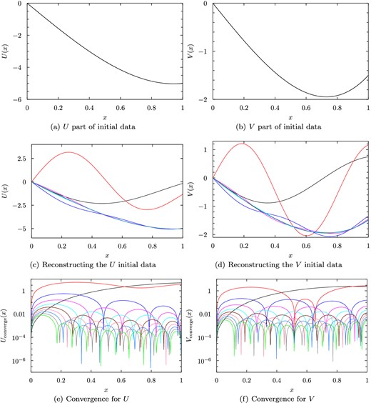
Figure A1.

Figure showing the reproduction of the initial data as a sum of eigenfunctions for the case b = 0.1. The U and V parts of the initial data are shown in the top row. In the middle row, the partial sums U^partial(N, x) and V^partial(N, x) are shown for N = 1 (black line) up to N = 10 (green line); the largest contribution is from the N = 3 eigenfunction (dark blue), which is the fluid-elastic hybrid mode. The bottom row plots the absolute value of the difference between the partial sums and the initial data, U^converge(N, x) and V^converge(N, x).

Open in new tab Download slide

To test how the partial sums converge with increased N, in the last row we have plotted the U (Fig. A1e) and V (Fig. A1f) parts of the absolute value of the difference between |$\boldsymbol {\xi }^{{\rm partial}}(N,x)$| and the initial data,

\begin{equation} \boldsymbol {\xi }^{{\rm converge}}(N,x)= \left|\boldsymbol {\xi }^{{\rm partial}}(N,x) - \boldsymbol {\xi }^{{\rm ID}}(x) \right|. \end{equation}

(A2)

We can see that the contributions become progressively smaller as N increases.

Next we consider the full problem with rotation, where we also have to reconstruct the velocity initial data as well as that for the displacement. The velocity field initial data |$\dot{\boldsymbol {\xi }}^{{\rm DC}}$| (equation 118) is made up from only one zeroth-order eigenfunction, the zero frequency n = 1 toroidal mode, and this mode has no corrections at first order in the rotation. This means that the velocity initial data can be reconstructed from one eigenfunction only, and this can be done with close to numerical precision.

As an example of the reconstruction for the displacement field initial data, Fig. A2 plots the U part of the fractional difference between the initial data and its reconstruction (equation 151), |U^reconstruct(n) − U^CD|/U^CD, for b = 10⁻² and t = 10⁻², with values of n between 1 and the cut-off N. We see that as with the special case of the glitch at zero spin, the initial data is not reproduced correctly until the hybrid mode is added, and the reconstruction then converges to the initial data as N is made larger.

$Figure showing the reconstruction of the initial data in the cases b = 10−1, 10−2 and 10−3, with t = 10−2. The U part of the fractional difference between the initial data and its reconstruction, |Ureconstruct(n) − UCD|/UCD, is plotted for values of n between 1 and the cut-off N. The initial data is not reproduced correctly until the hybrid mode is added, and the reconstruction then converges to the initial data as N is made larger.$

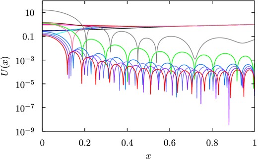
Figure A2.

Figure showing the reconstruction of the initial data in the cases b = 10⁻¹, 10⁻² and 10⁻³, with t = 10⁻². The U part of the fractional difference between the initial data and its reconstruction, |U^reconstruct(n) − U^CD|/U^CD, is plotted for values of n between 1 and the cut-off N. The initial data is not reproduced correctly until the hybrid mode is added, and the reconstruction then converges to the initial data as N is made larger.

Open in new tab Download slide

APPENDIX B: ORTHOGONALITY OF EIGENFUNCTIONS FOR A SPHERICAL ELASTIC STAR

Here, we show that the eigenfunctions for our background model Star S, a homogeneous, incompressible elastic star, are orthogonal. The corresponding result has been shown for the cases of non-radial oscillations of stationary, perfect fluid stars (Chandrasekhar 1964; Lynden-Bell & Ostriker 1967; Friedman & Schutz 1978) and also for the incompressible fluid star (Chandrasekhar & Lebovitz 1964). We will follow a similar method here, and show that our operator C₍₀₎ (equation 107) is symmetric,

\begin{equation} \left\langle \boldsymbol {\eta }, C_{(0)}\boldsymbol {\xi }\right\rangle = \left\langle \xi , C_{(0)}\boldsymbol {\eta } \right\rangle , \end{equation}

(B1)

given the boundary conditions (82). Writing the inner product out in full,

\begin{equation} \left\langle \boldsymbol {\eta }, C_{(0)}\boldsymbol {\xi }\right\rangle = \int _V\nabla _j \tau {_i^j}\eta ^i \mathrm{d}V + \int _V\rho (\nabla _i\delta \Phi )\eta ^i \mathrm{d}V. \end{equation}

(B2)

It is then sufficient to show that both terms of the right-hand side are symmetric in ξⁱ and ηⁱ, given our boundary conditions. We will only show this for the first term, as the second term is identical to that for the incompressible fluid star. Integrating by parts,

\begin{equation} \int _V\nabla _j \tau {_i^j}\eta ^i \mathrm{d}V = -\int _V (\nabla _j\eta ^i)\tau {_i^j} \mathrm{d}V + \int _{\mathrm{\partial} V} \eta ^i \tau {_i^j} \mathrm{d}S_j. \end{equation}

(B3)

For the surface term, we can use the boundary conditions (82) to substitute in τ_ij, so that

\begin{equation} \int _{\mathrm{\partial} V} \eta ^i \tau {_i^j} \mathrm{d}S_j = \int _{\mathrm{\partial} V} \eta ^r \xi ^r \frac{\mathrm{d} p}{\mathrm{d} r} \, \mathrm{d}S_r, \end{equation}

(B4)

where we have used the spherical symmetry of the background star. This term is symmetric in ξ and η. For the volume term, we expand out |$\tau {_i^j}$| so that

\begin{equation} -\int _V (\nabla _j\eta ^i)\tau {_i^j} \mathrm{d}V = -\int _V (\nabla _j\eta ^i)(-\delta p \delta {_i^j} + \mu \nabla _i\xi ^j + \mu \nabla ^j\xi _i) \mathrm{d}V. \end{equation}

(B5)

The first term of this is zero by incompressibility, while the third term is already symmetric. To deal with the second term, we will integrate half by parts with respect to ∇_i, and half with respect to ∇_j, so that

\begin{equation} -\int _V \mu (\nabla _j\eta ^i)\left(\nabla _i\xi ^j\right) \mathrm{d}V = \frac{1}{2}\left[\int _V \eta ^i\nabla _j(\mu \nabla _i\xi ^j)\; \mathrm{d}V -\int _{\mathrm{\partial} V} \mu \eta ^i\nabla _i\xi ^j \mathrm{d}S_j +\int _V \xi ^j\nabla _i(\mu \nabla _j\eta ^i)\; \mathrm{d}V -\int _{\mathrm{\partial} V} \mu \xi ^j\nabla _j\eta ^i \mathrm{d}S_i\right]. \end{equation}

(B6)

Using the product rule on the volume terms, this becomes

\begin{eqnarray} -\int _V \mu (\nabla _j\eta ^i)\left(\nabla _i\xi ^j\right) \mathrm{d}V &=& \frac{1}{2}\left[\int _V (\nabla _j\mu )\eta ^i(\nabla _i\xi ^j)\; \mathrm{d}V +\int _V \mu \eta ^i\nabla _j \nabla _i\xi ^j \mathrm{d}V +\int _V (\nabla _i \mu )\xi ^j( \nabla _j\eta ^i) \mathrm{d}V +\int _V \mu \xi ^j\nabla _i \nabla _j\eta ^i \mathrm{d}V \right.\nonumber\\ && \left.-\int _{\mathrm{\partial} V} \mu \eta ^i\nabla _i\xi ^j \mathrm{d}S_j -\int _{\mathrm{\partial} V} \mu \xi ^j\nabla _j\eta ^i \mathrm{d}S_i\right]. \end{eqnarray}

(B7)

The shear modulus μ is constant over the surface of the star, and so its derivative ∇_iμ is non-zero only at the surface,

\begin{equation} \nabla _i\mu = -\mu \delta (r-R)\hat{r}_i. \end{equation}

(B8)

The terms containing ∇_iμ then cancel with the two surface terms to leave

\begin{equation} -\int _V \mu (\nabla _j\eta ^i)\left(\nabla _i\xi ^j\right) \mathrm{d}V = \int _V \mu \eta ^i\nabla _j \nabla _i\xi ^j \mathrm{d}V + \int _V \mu \xi ^j\nabla _i \nabla _j\eta ^i. \end{equation}

(B9)

These two terms are zero, as can be seen by commuting ∇_i and ∇_j and using the incompressibility condition, so that finally we have

\begin{equation} \int _V\nabla _j \tau {_i^j}\eta ^i \mathrm{d}V = \int _{\mathrm{\partial} V} \eta ^r \xi ^r \frac{\mathrm{d} p}{\mathrm{d} r} \, \mathrm{d}S_r -\int _V \mu (\nabla _j\eta ^i)(\nabla ^j\xi _i). \end{equation}

(B10)

We have now shown that C₍₀₎ is a symmetric operator, and so the eigenvalues of a self-gravitating elastic incompressible star are orthogonal with respect to A₍₀₎ ≡ ρ:

\begin{equation} \langle \eta , A_{(0)}\xi \rangle = 0, \quad \omega ^2_\eta \ne \omega ^2_\xi . \end{equation}

(B11)

Download all slides

Month:	Total Views:
January 2017	2
March 2017	3
April 2017	4
May 2017	1
June 2017	1
July 2017	4
August 2017	1
November 2017	9
January 2018	12
February 2018	10
March 2018	10
April 2018	21
May 2018	13
June 2018	13
July 2018	26
August 2018	9
September 2018	19
October 2018	16
November 2018	27
December 2018	6
January 2019	16
February 2019	13
March 2019	10
April 2019	16
May 2019	5
June 2019	5
July 2019	8
August 2019	13
September 2019	4
October 2019	5
November 2019	16
December 2019	4
January 2020	11
February 2020	6
March 2020	17
April 2020	9
May 2020	7
June 2020	7
July 2020	12
August 2020	9
September 2020	14
October 2020	9
November 2020	12
December 2020	16
January 2021	12
February 2021	22
March 2021	12
April 2021	6
May 2021	9
June 2021	8
July 2021	3
August 2021	3
September 2021	14
October 2021	14
November 2021	14
December 2021	5
January 2022	6
February 2022	8
March 2022	5
April 2022	24
May 2022	10
June 2022	11
July 2022	19
August 2022	11
September 2022	12
October 2022	13
November 2022	14
December 2022	8
January 2023	5
February 2023	24
March 2023	25
April 2023	11
May 2023	10
June 2023	16
July 2023	4
August 2023	14
September 2023	10
October 2023	14
November 2023	7
December 2023	24
January 2024	14
February 2024	12
March 2024	11
April 2024	23
May 2024	26
June 2024	9
July 2024	8
August 2024	10
September 2024	14
October 2024	18
November 2024	17
December 2024	14
January 2025	16
February 2025	11
March 2025	11
April 2025	2
May 2025	9

Article Contents

Developing a model for neutron star oscillations following starquakes

Abstract

1 INTRODUCTION

2 THE STARQUAKE TOY MODEL

2.1 Plan of the calculation

3 ENERGY ESTIMATES FOR THE MODEL

3.1 Energies released in the starquake

3.2 Estimates for solid quark stars

4 CONSTRUCTION OF THE INITIAL DATA

5 OSCILLATION MODES OF THE ROTATING STAR

5.1 Oscillation modes of the spherical background star

5.2 Rotating star

6 PROJECTING THE INITIAL DATA

6.1 Special case: glitch at zero spin

6.2 The general case: glitch at arbitrary spin

6.3 Results of the projection

7 CONCLUSIONS

REFERENCES

APPENDIX A: RECONSTRUCTION OF THE INITIAL DATA

APPENDIX B: ORTHOGONALITY OF EIGENFUNCTIONS FOR A SPHERICAL ELASTIC STAR

Citations

Views

Altmetric

Email alerts

Astrophysics Data System

Citing articles via

Latest

Most Read

Most Cited

Article Contents

Developing a model for neutron star oscillations following starquakes Free

Abstract

1 INTRODUCTION

2 THE STARQUAKE TOY MODEL

2.1 Plan of the calculation

3 ENERGY ESTIMATES FOR THE MODEL

3.1 Energies released in the starquake

3.2 Estimates for solid quark stars

4 CONSTRUCTION OF THE INITIAL DATA

5 OSCILLATION MODES OF THE ROTATING STAR

5.1 Oscillation modes of the spherical background star

5.2 Rotating star

6 PROJECTING THE INITIAL DATA

6.1 Special case: glitch at zero spin

6.2 The general case: glitch at arbitrary spin

6.3 Results of the projection

7 CONCLUSIONS

REFERENCES

APPENDIX A: RECONSTRUCTION OF THE INITIAL DATA

APPENDIX B: ORTHOGONALITY OF EIGENFUNCTIONS FOR A SPHERICAL ELASTIC STAR

Citations

Views

Altmetric

Email alerts

Astrophysics Data System

Citing articles via

Latest

Most Read

Most Cited

This Feature Is Available To Subscribers Only

Developing a model for neutron star oscillations following starquakes