


Abstract
The 30-Hz rotation rate of the Crab pulsar has been monitored at Jodrell Bank Observatory since 1984 and by other observatories before then. Since 1968, the rotation rate has decreased by about 0.5 Hz, interrupted only by sporadic and small spin-up events (glitches). 24 of these events have been observed, including a significant concentration of 15 occurring over an interval of 11 yr following MJD 50000. The monotonic decrease of the slowdown rate is partially reversed at glitches. This reversal comprises a step and an asymptotic exponential with a 320-d time constant, as determined in the three best-isolated glitches. The cumulative effect of all glitches is to reduce the decrease in slowdown rate by about 6 per cent. Overall, a low mean braking index of 2.342(1) is measured for the whole period, compared with values close to 2.5 in intervals between glitches. Removing the effects of individual glitches reveals an underlying power-law slowdown with the same braking index of 2.5. We interpret this value in terms of a braking torque due to a dipolar magnetic field in which the inclination angle between the dipole and rotation axes is increasing. There may also be further effects due to a monopolar particle wind or infalling supernova debris.
1 INTRODUCTION
For most pulsars, evaluation of the rotational slowdown law is confined to measurement of the rotational frequency ν and its first derivative |$\dot{\nu }$|. For old pulsars, the second derivative |$\ddot{\nu }$| expected from equation (3) is usually immeasurably small, while in many younger pulsars any secular behaviour is often confused by unpredictable changes in rotation rate, in the form of either timing noise or glitches. Timing noise is seen as slow quasi-random changes in rotation rate and arises from magnetospheric instabilities (Lyne et al. 2010), while glitches are almost instantaneous increases in rotation rate, often followed by some associated transient behaviour and have their origin in the neutron star interior (Espinoza et al. 2011a).
Because of these effects, values of braking index have been reliably established for only eight pulsars. For the Crab pulsar, |$\ddot{\nu }$| has been measured between glitches (Lyne, Pritchard & Smith 1993), leading to an observed value nobs = 2.51(1), significantly less than the value of n = 3 expected for braking by magnetic dipole radiation. The same is true for all the other seven pulsars (Table 1). These results indicate that the physical process causing the slowdown is not just simple dipolar electromagnetic radiation.
Measured braking indices for young pulsars.
| PSR | n | Reference |
|---|---|---|
| B0531+21(Crab) | 2.51(1) | Lyne et al. (1993) |
| B0540−69 | 2.14(1) | Livingstone et al. (2007) |
| B0833−45(Vela) | 1.4(2) | Lyne et al. (1996) |
| J1119−6127 | 2.684(2) | Weltevrede, Johnston & Espinoza (2011) |
| B1509−58 | 2.839(1) | Livingstone et al. (2007) |
| J1734−3333 | 0.9(2) | Espinoza et al. (2011b) |
| J1833−1034 | 1.857(1) | Roy, Gupta & Lewandowski (2012) |
| J1846−0258 | 2.65(1) | Livingstone et al. (2007) |
In this paper, we report on the measurement and analysis of the rotation rate of the Crab pulsar from 1968 to 2013. This 45-yr time baseline amounts to about 5 per cent of the pulsar lifetime and allows the spin-down of the Crab pulsar to be described over a period which includes many glitches and provides more details of the cumulative effect that they have on the long-term spin-down (Lyne et al. 1993; Smith & Jordan 2003). Elsewhere, the same data have been used to examine the statistics and physical details of the glitches (Espinoza et al. 2014) and to study the evolution of the radio pulse emission over this time (Lyne et al. 2013) to enable a comprehensive picture of the evolution of the pulsar.
2 OBSERVATIONS AND BASIC ANALYSIS
The rotation of the Crab pulsar has been monitored by daily observations at Jodrell Bank Observatory since 1984, mainly using the 13-m radio telescope at 610 MHz (Lyne, Pritchard & Smith 1988, 1993). Regular observations with the 76-m Lovell telescope at around 1400–1700 MHz, designed to monitor any changes in dispersion measure, also contribute to the data set.
These data have been supplemented with earlier observations taken at Arecibo (Gullahorn et al. 1977) and in the optical at Princeton (Groth 1975) and Hamburg (Lohsen 1981). There are no observations available between 1979 February and 1982 February, this being the only significant gap with no data. There are in total approximately 11 000 times of arrival (TOAs) and together the measurements comprise a record of the rotation of the pulsar over a total of 45 yr from 1968 November to 2013 December.
In order to study the long-term rotational history of the pulsar, we have used standard procedures to reduce the TOAs to the barycentre of the Solar system. We have then fitted values of the rotation frequency ν and its first two derivatives |$\dot{\nu }$| and |$\ddot{\nu }$| over time spans of approximately 100 d. Such analyses were repeated with the central reference time advancing by typically 50 d between analyses. Close to glitches, the time spans were adjusted in such a way that no analysis was performed over a glitch, so that one analysis ended and another started close to the epoch of the glitch.
These time sequences of rotational frequencies and first derivatives provide the main forms of the data that we use to study the long-term behaviour of the pulsar in this paper. Figs 1(a) and 2(a) illustrate the evolution of the rotational frequency ν(t) and slowdown rate |$\dot{\nu }({\rm t})$| over the 45 yr. The rotational slowdown of the pulsar is evident in Fig. 1(a), falling by about 0.5 Hz during this time. The slowdown rate (Fig. 2 a) also shows a general reduction in magnitude with time, but there are also considerable long-term effects resulting from glitches, which we investigate further in a later section.
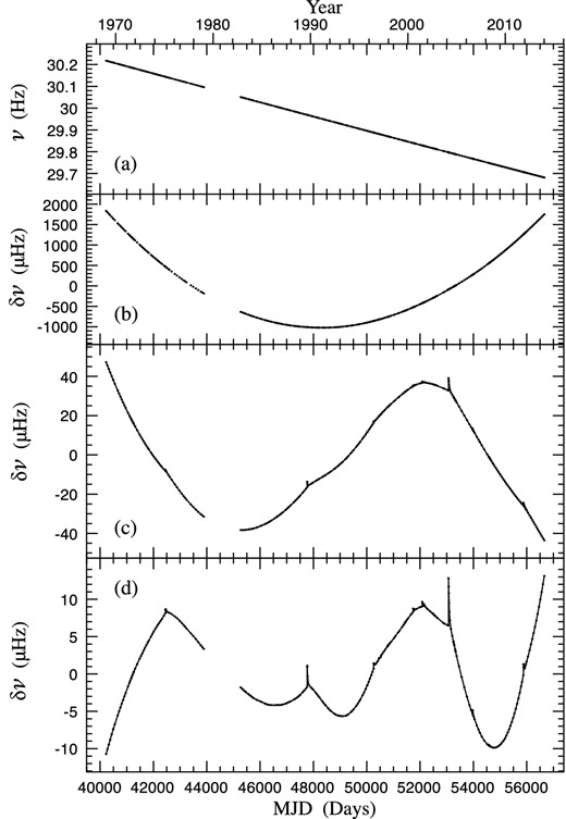
The spin-frequency history of the Crab pulsar over 45 years. (a) The observed spin frequency ν determined from fits to 100-d data sets every 50 d, showing the monotonic slowdown of the pulsar. (b), (c) and (d) The frequency residuals δν after fitting to the values in (a) simple slowdown models involving frequency and, respectively, one, two and three spin-frequency derivatives in the Taylor series of equation (5). The fitted values of ν0, |$\dot{\nu }_0$|, |$\ddot{\nu }_0$| and |$\stackrel{...}{\nu }_0$| for (d) are given in Table 2.
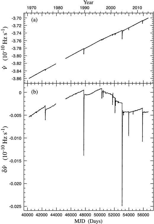
The slowdown rate |$\dot{\nu }$| of the Crab pulsar over 45 years. (a) Observed values of the first derivative |$\dot{\nu }$| determined from fits to 100-d data sets every 50 d. The magnitude of the slowdown rate |$\vert \dot{\nu }\vert$| is decreasing overall, with small step increases at the glitches. (b) Frequency derivative residuals |$\delta \dot{\nu }$| on an expanded scale, obtained by subtracting from (a) a linear model using the values of the first two frequency derivatives given in Table 2.
Observed and derived parameters for the Crab pulsar. The spin parameters were obtained by fitting a three-derivative Taylor series to the frequency data presented in Fig. 1(a). The standard errors determined in the analysis are given in parentheses after the values and are in units of the least significant digit.
| Parameter | Value |
|---|---|
| Data span (MJD) | 40175–56665 |
| Epoch t0 (MJD) | 48442.5 |
| ν0 (Hz) | 29.946 923(1) |
| |$\dot{\nu }_0$| (10−10 Hz s−1) | −3.775 35(2) |
| |$\ddot{\nu }_0$| (10−20 Hz s−2) | 1.1147(5) |
| |$\stackrel{...}{\nu }_0$| (10−30 Hz s−3) | −2.73(4) |
| rms residual (Hz) | 0.000 0058 |
| Maximum frequency residual (Hz) | 0.000 013 |
| Mean braking index n | 2.342(1) |
Using equation (3) and the values in Table 2, a braking index n = 2.342(1) is obtained. Using this braking index in equation (4), it is found that the expected value of |$\stackrel{...}{\nu }$| is −0.52 × 10⁻³⁰ Hz s−3, which is about one-fifth of the measured value. This shows that the general long-term slowdown of the Crab pulsar is not a simple power law. We show later that removal of the effects of glitches brings the slowdown close to a simple power law.
Extrapolating the Taylor series back in time to investigate the behaviour in earlier years should evidently be approached with caution, but we remark that the series indicates an original rotation rate of 58 Hz (a period of 17 ms) at birth in ad 1054.
3 THE 24 GLITCHES
The monotonic rotational slowdown of the Crab pulsar seen in Fig. 1 is occasionally reversed discontinuously at a glitch, in which ν increases by a small step Δν of the order of 10−9ν to 10−7ν, followed by a nearly complete recovery within about 20 d of the event. The magnitude of the slowdown rate |$\vert \dot{\nu }\vert$| (Fig. 2) also presents an initial step increase at a glitch, again partially reversing the long-term trend and showing the corresponding short-term recovery (Lyne, Pritchard & Smith 1993; Wong, Backer & Lyne 2001). However, in contrast with the relaxation in ν, the recovery in slowdown rate is not complete and a persistent step (|$\Delta \dot{\nu }_{\rm p}$|) is commonly observed after glitches. First remarked upon by Gullahorn et al. (1977) and Demiański & Prószyński (1983) in relation to the glitch of 1975, these persistent steps are a general feature of glitches in this pulsar and have an appreciable effect on the overall slowdown behaviour.
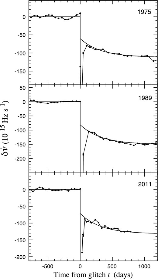
The variation in slowdown rate |$\dot{\nu }$| of the Crab pulsar near to the three large isolated glitches which occurred in 1975, 1989 and 2011. In each case, the frequency derivative residuals |$\delta \dot{\nu }$| were obtained relative to a linear model involving the first two frequency derivatives fitted to |$\dot{\nu }$| over the 800 d preceding the glitch, which occurred at day 0. Each glitch is followed instantly by a large negative transient (increase in magnitude) in |$\dot{\nu }$|. The main transient behaviour ceases after about 100 d, revealing a persistent negative offset which continues to increase in a quasi-exponential manner on a time-scale of around 320 d. The smooth lines are the fits to the post-glitch data described by equation (6).
We now regard this as an intrinsic component of all glitches, although for many it is often obscured by the recovery from previous glitches or the occurrence of later glitches. The asymptotic exponential component has a time-scale of 320 ± 20 d and comprises 46 per cent, or almost half, of the total increase of slowdown rate. In what follows, we assume that these values apply to all glitches in the Crab pulsar.
Table 3 lists 24 glitches, giving the date and MJD of occurrence, the step change Δν, the fractional value Δν/ν and the persistent change of slowdown rate |$\Delta \dot{\nu }_{\rm p}$|. This is a robust list which includes all glitches for which Δν > 0.01 μHz. Any glitches smaller than this are of similar size to the period variations produced by the noise present in the data. Any glitch which may have occurred during the gap in observations in 1981 left no obvious change in slowdown rate, and would presumably have been small and would not affect the results of our analysis. Glitch epochs and frequency step sizes were taken from Espinoza et al. (2011a,c). The sequence of glitches is illustrated in Fig. 4(a), which shows the date of occurrence and the size Δν of each glitch (on a logarithmic scale). Note particularly the pattern of substantially increased activity from MJD ∼ 50000 to MJD ∼ 54000 (years 1995–2006). A histogram of glitch sizes Δν is shown in Fig. 5(a). Espinoza et al. (2014) have analysed the Jodrell Bank data on the Crab pulsar and conclude that the decrease in numbers of glitches towards smaller sizes is intrinsic and is not related to the detection capabilities.
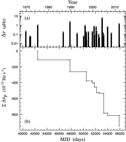
Glitches in the Crab pulsar. (a) The distribution in time and magnitude of the steps Δν in spin frequency of the 24 glitches in Table 3. (b) The cumulative effect of the persistent steps in slowdown rate |$\Delta {\dot{\nu }}_{\rm p}$| at the glitches.
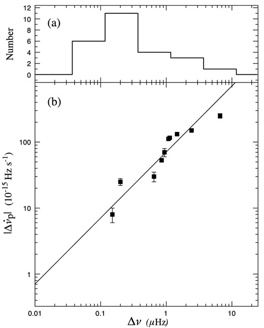
Glitch sizes. (a) Histogram of frequency steps Δν on a logarithmic scale for the 24 glitches in Table 3. (b) The inter-dependence of the persistent change in slowdown rate |$|\Delta \dot{\nu }_{\rm p}|$| and the step change in rotation frequency Δν for 10 glitches. The diagonal line has a slope of unity.
The steps in rotation rate and slowdown rate for the 24 glitches observed between 1968 and 2013. This table is derived from Espinoza et al. (2014).
| Date | MJD | |$\frac{\Delta \nu }{\nu }$| | Δν | |$\Delta \dot{\nu }_p$| |
|---|---|---|---|---|
| (d) | 10−9 | (μHz) | (10−15 s−2) | |
| 1969 September | 40491.84(3) | 7.2(4) | 0.22(1) | – |
| 1971 July | 41161.98(4) | 1.9(1) | 0.057(4) | – |
| 1971 October | 41250.32(1) | 2.1(1) | 0.062(3) | – |
| 1975 February | 42447.26(4) | 35.7(3) | 1.08(1) | −112(2) |
| 1986 August | 46663.69(3) | 6(1) | 0.18(2) | – |
| 1989 August | 47767.504(3) | 81.0(4) | 2.43(1) | −150(5) |
| 1992 November | 48945.6(1) | 4.2(2) | 0.13(1) | – |
| 1995 October | 50020.04(2) | 2.1(1) | 0.063(2) | – |
| 1996 June | 50260.031(4) | 31.9(1) | 0.953(4) | – |
| 1997 January | 50458.94(3) | 6.1(4) | 0.18(1) | −116(5)a |
| 1997 December | 50812.59(1) | 6.2(2) | 0.19(1) | – |
| 1999 October | 51452.02(1) | 6.8(2) | 0.20(1) | −25(3) |
| 2000 July | 51740.656(2) | 25.1(3) | 0.75(1) | – |
| 2000 September | 51804.75(2) | 3.5(1) | 0.105(3) | −53(3)a |
| 2001 June | 52084.072(1) | 22.6(1) | 0.675(3) | – |
| 2001 October | 52146.7580(3) | 8.87(5) | 0.265(1) | −70(10)a |
| 2002 August | 52498.257(2) | 3.4(1) | 0.101(2) | – |
| 2002 September | 52587.20(1) | 1.7(1) | 0.050(3) | −8(2)a |
| 2004 March | 53067.0780(2) | 214(1) | 6.37(2) | – |
| 2004 September | 53254.109(2) | 4.9(1) | 0.145(3) | – |
| 2004 November | 53331.17(1) | 2.8(2) | 0.08(1) | −250(20)b |
| 2006 August | 53970.1900(3) | 21.8(2) | 0.65(1) | −30(5) |
| 2008 April | 54580.38(1) | 4.7(1) | 0.140(4) | – |
| 2011 November | 55875.5(1) | 49.2(3) | 1.46(1) | −132(5) |
aIncorporates the persistent step of the previous glitch.
bIncorporates the persistent steps of the previous two glitches.
The persistent steps in frequency derivative were estimated by fitting a function of the form given by equation (6) to the observed |$\dot{\nu }$| data centred on the glitch epoch. In order to avoid contamination by short-term glitch transient recoveries, data taken within 90 d following each glitch were not used. In some cases, the step is very small and no significant measurement was possible. In other cases, because of the presence of other nearby glitches, the available data points were insufficient to perform the measurement, although in a few cases it was possible to measure the combined effect of two or three closely separated glitches (Table 3). Without being extremely precise, this method effectively measures the basic trends we are studying and it is not affected by the necessary assumptions of more complicated models. Our values are roughly consistent with existent measurements using such models (e.g. Wong et al. 2001; Wang et al. 2012).
The persistent slowdown increase is usually attributed to a reduction in effective moment of inertia due to pinning of neutron superfluid vortices to other internal components. Because a rotating superfluid slows down only if its vortices are allowed to move apart, the pinning of some vortices decouples a fraction of the superfluid from the rest of the star and reduces the effective moment of inertia of the rotating star. Equation (7) indicates that the re-pinning of vortices is more effective after larger glitches.
We offer no explanation for the surprising phenomenon of the long-term asymptotic increase in |$\dot{\nu }$| and continue to view all increases of slowdown rate at glitches as decreases in effective moment of inertia, presumably due to vortex pinning. We note that if there is no relaxation in this cumulative pinning, the proportional change in moment of inertia has amounted to 0.3 per cent in 45 years. We remark that such a large rate of change cannot persist for more than a few thousand years, by which time a large proportion of the effective moment of inertia of the neutron star would have disappeared.
Melatos, Peralta & Wyithe (2008) include the Crab pulsar glitches in a comprehensive analysis of the statistics of the distributions of size and intervals between glitches, testing the hypothesis that these are determined by a random process of self-organized criticality. The incidence of glitches in most pulsars appears to be random, and Wang et al. (2012) show that the distribution of interval times in the Crab pulsar is Poissonian, although some pulsars show a quasi-periodicity (Link, Epstein & Lattimer 1999; Melatos et al. 2008; Wang et al. 2012).
We nevertheless draw attention to the cluster of 15 glitches between MJD 50000 and 54000 seen in Fig. 4, which suggests that there may be an extra complexity in the system. We require a statistical test for the hypothesis that this cluster was a chance concentration of glitches which occurred at random. The Wang et al. (2012) test was not sensitive to clustering, which is better revealed by the distribution of intervals between all glitches, rather than only consecutive ones. We therefore compare the observed distribution of intervals between all glitches with those from simulated glitch sequences and show that the probability that the observed distribution is random is low.
We confined our analysis to the 20 glitches which occurred in the last 30 years since high-cadence monitoring commenced in 1984 January. As explained in Espinoza et al. (2014), the data in this period constitute a uniform set and are complete, indicating a mean rate of 0.67 glitches per year. The bold line in Fig. 6 shows the cumulative distribution of all 190 glitch separation times in this set of data. We then generated 10 000 simulated distributions of 20 events, each occurring at a random time within a 30-yr period; in Fig. 6, we show 100 of these realizations (randomly picked) for comparison with the observed distribution.
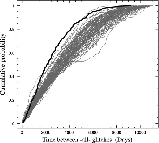
The cumulative distribution of intervals between all 20 glitches occurring between MJD 46000 and MJD 56600, as observed (bold line) and in 100 random simulations.
The curve derived from the observed data lies on the outside of the spread of curves from the simulations, indicating a low probability that the observed cluster was a random occurrence. In particular, there is an excess of small separation times in the observed cumulative distribution, which is therefore steeper than most of the simulated distributions. This indicates that the glitches are more clustered than can be expected from a random occurrence of glitches. We also compared the means of the separation times in the distributions; the mean of the 190 observed glitch separation times was less than the mean in all except 52 (0.5 per cent) of the 10 000 simulated distributions. We therefore conclude that it is unlikely that the cluster of glitches is a statistical accident. We note that the 11-yr period of the cluster coincides with a period of an anomaly in the underlying slowdown rate, which is seen in Fig. 7 and will be discussed in the next section.
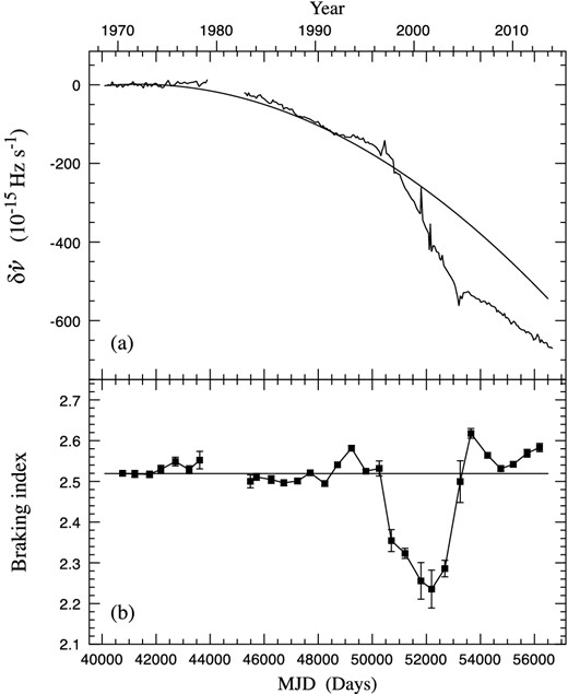
The underlying slowdown of the Crab pulsar after removal of the effects of the glitches. (a) The frequency derivative residuals |$\delta \dot{\nu }$| obtained by subtracting from |$\dot{\nu }$| data the persistent steps |$\Delta \dot{\nu }_{\rm p}$| at the glitches given in Table 3, removing short-term glitch transients by excluding data within 90 d following each glitch, and by removing the main linear trend as measured from the start to MJD 50458. The smooth curve is the expected behaviour during this era for a constant value of n = 2.519, showing a curvature corresponding to a value of |$\stackrel{...}{\nu } = -0.636\times 10^{-30}$| Hz s−3 as calculated from equation (4). (b) The underlying braking index of the Crab pulsar using equation (3), evaluated over sections of 1000 d at 500-d intervals. The values of ν and |$\dot{\nu }$| are the mean values of the data in each interval in Figs 1(a) and 2(a), and |$\ddot{\nu }$| is taken from the slope of the corresponding data in (a). The horizontal line at n = 2.519 corresponds to the curve in (a).
4 THE EFFECT OF GLITCHES ON THE SLOWDOWN
Fig. 4(b) shows the cumulative effect of the steps |$\Delta \dot{\nu }_{\rm p}$| at the 16 glitches for which this quantity was measured. The total cumulative effect over 45 years is an increase in slowdown rate |$\vert \Sigma \Delta \dot{\nu }_{\rm p}\vert$| of 946(25) × 10−15 Hz s−1. The small but appreciable overall negative contribution made by the glitches to the second derivative |$\ddot{\nu }$| may be evaluated by dividing the total sum by the time interval, giving a value of −0.066(2) × 10−20 Hz s−2, which is approximately 6 per cent of the second derivative |$\ddot{\nu }$| evaluated from the long-term analysis (Table 2).
We now address the notion that the slowdown is an underlying steady phenomenon with superimposed cumulative steps in the slowdown rate caused by glitches. If the persistent steps |$\Delta \dot{\nu }_{\rm p}$|, as tabulated in Table 3 and with the form described by equation (6), are removed from the |$\dot{\nu }$| data, we obtain a smoother, ‘corrected’ |$\dot{\nu }$| evolution which shows the underlying slowdown. Fig. 7(a) shows frequency derivative residuals obtained by removing from the corrected |$\dot{\nu }$| data a new linear two-term Taylor series fitted to the restricted 6-yr span up to MJD 42447, this being the epoch of the 1975 glitch. This fit yields values of |$\dot{\nu }=-3.847\,96(1)\times 10^{-10}$| Hz s−1 and |$\ddot{\nu }=1.236(1)\times 10^{-20}$| Hz s−2 at MJD 41338.67. We now find from equation (3) that during this span, the braking index was n = 2.519(2), and from equation (4) the expected value of |$\stackrel{...}{\nu } = -0.636(1)\times 10^{-30}$| Hz s−3. The smooth curve in Fig. 7(a) is the calculated variation in |$\dot{\nu }$| including the curvature due to this term, and in general is seen to track the data well.
However, at around MJD 50000, the slope in Fig. 7(a) changes abruptly, recovering at around MJD 54000, after an accumulated offset in |$\dot{\nu }$|, to approximately the expected slope. This is the same 11-yr span that contains the large concentration of glitches. The accumulated deviation in this 11-yr span amounts to ∼−200 × 10−15 Hz s−1, and is in addition to the ∼−522 × 10−15 Hz s−1 already accounted for by the observed persistent glitch contributions |$\Delta \dot{\nu }_{\rm p}$| in this period, and may be compared with the total change during this time of ∼3500 × 10−15 Hz s−1 due to the underlying slowdown. It seems unlikely that the deviation can be due to glitches which are below the threshold of our measurements, since Fig. 5(a) shows a deficit of small glitches (Espinoza et al. 2014). More likely, the accumulated deviation is due to a phenomenon related to glitches which is not reflected in our present model.
The variations in |$\delta \dot{\nu }$| may also be interpreted as changes in the underlying value of the braking index n with time. These changes are summarized in Fig. 7(b), in which the value of the braking index is close to 2.5 throughout most of the 45 years, except for the period of high glitch activity from MJD 50000 to 54000, when it takes a value of about 2.3.
We remark that the process of separating the effects of glitches from an underlying steady rotational evolution provides a good description of the overall behaviour, with braking index n = 2.5. The small effect on the index seen in Fig. 7(b) remains unexplained.
5 THE SLOWDOWN POWER LAW
Why is the braking index different from 3, as expected from equation (1) for energy loss through electromagnetic dipole radiation? Either this equation is inadequate because angular momentum is also lost through a mechanical process such as an outflowing jet or interaction with an external fall-back disc of supernova remains (Menou, Perna & Hernquist 2001), or one or more of the parameters I, M or α of the equation is changing with time. These two categories might be called the unipolar and dipolar approaches in which the loss of angular momentum may lead to very different slowdown laws |$\dot{\nu }\ \propto \nu$| and |$\dot{\nu }\propto \nu ^3$|, respectively. As pointed out by Harding, Contopoulos & Kazanas (1999), Xu & Qiao (2001) and Chen & Li (2006), a combination of both processes could account for the observed low braking indices of young pulsars.
5.1 The wind component
The Crab pulsar, along with other young pulsars, generates a powerful particle stream whose effect is observed as a wind nebula (e.g. Gaensler & Slane 2006). The possible effect of angular momentum carried away by this particle stream has been much debated, following Michel & Tucker (1969) who pointed out that if the slowdown were predominantly due to wind, the torque would follow the first rather than the third power of the rotation rate. Other values of braking index of less than 3 due to particle flows have also been suggested (e.g. Wu, Xu & Gil 2003). An alternative approach by Menou et al. (2001) suggests that interaction between the rotating pulsar and an accretion disc of infalling supernova remains, forming outside the magnetosphere but coupled by a propeller torque, would lead to a similar slowdown law. Yan, Perna & Soria (2012) consider the effect of this process on the timing properties of old as well as young pulsars.
If the wind (or the disc) was to be responsible for the whole of the difference between ndip = 3, the expected value from magnetic dipole braking, and nobs, the observed value, then equation (10) shows that for nobs = 2.5, the wind accounts for approximately one-third of the slowdown torque. A more precise modelling of the effect of the wind or disc might lead to a more accurate assessment of this proportion. For the Vela pulsar, the very low value of nobs = 1.4 suggests that the wind is responsible for 4/5 of the slowdown torque.
5.2 A changing magnetic dipole
The overall changes in the Crab slowdown are too large to be explained by simple changes in ellipticity and the consequent changes in the moment of inertia I of a rotating ellipsoid. An apparent reduction in I might however be due to a continuous decoupling of the interior produced by an accumulation of pinned vortices in reservoirs (Alpar et al. 1996; Ho & Andersson 2012), eventually locking up a substantial fraction of the superfluid. Such a process would eventually be limited by the available superfluid, which is usually considered to be the superfluid in the neutron-rich inner crust. It seems unlikely that the process could persist long enough to explain the low braking index of older pulsars such as the Vela pulsar.
Several authors, notably (Blandford & Romani 1988; Allen & Horvath 1997; Chen, Ruderman & Zhu 1998; Lyne 2004; Espinoza et al. 2011b), have remarked that a low braking index might be due to an increasing dipolar magnetic field, or to an increasing inclination angle α. Evidence for a secular increase in α has been presented by Lyne et al. (2013). From observations of the profile of the radio pulse over 22 years, they find an increase in the component separation amounting to 6 × 10⁻³ deg yr−1. They remark that this can be attributed to a similar rate of increase in α, which for α = 45 deg would account for the low value of the braking index. Using the long-term value of nobs = 2.50, they found that the changing α gives a value of |$\dot{\kappa }/\kappa =2.6\times 10^{-4}$| yr−1, which could account for the observed rate of change.
However, although the secular change in α may well be sufficient to account for the whole of the reduction in the value of the braking index below 3, it should be noted that the determination of |$\dot{\alpha }$| from the observation of the separation of the components of the pulse profile is model dependent. Hence, the actual contribution is uncertain and it is also likely that the relative contributions of the different processes discussed above may be evolving with time. Further possibilities are models of pulsar magnetospheres which recognize an inner region corotating with the star and which can lead to n < 3 when the evolution of this region's size changes at a different rate to the constantly growing light cylinder region (Melatos 1997; Bucciantini et al. 2006; Contopoulos & Spitkovsky 2006).
6 LONG-TERM EVOLUTION AND THE |$P{\rm -}\dot{P}$| DIAGRAM
The departure from simple magnetic dipole slowdown is illustrated dramatically in Fig. 8. This shows a section of the familiar |$P{\rm -}\dot{P}$| diagram, a log–log plot on which it is customary to plot all known pulsars. As a pulsar ages, it moves from left to right across the diagram, following a path whose slope 2 − n depends on the braking index. For n = 3, the slope is −1. For the Crab pulsar, for which the mean value of n = 2.342, the slope is ∼−0.34, representing the general movement of the Crab pulsar on the diagram. However, between glitches the evolution is with a slope of −0.5, corresponding to n = 2.5. If the wind model is correct, the monopole term will eventually dominate and the path across the |$P{\rm -}\dot{P}$| diagram will turn upwards towards a slope of +1. As pointed out by Alvarez & Carramiñana (2004), this leads into a region of the diagram where no pulsars have been detected; however, it does lead towards the magnetars (Espinoza et al. 2011b). Harding et al. (1999) remark on the possibility that the high slowdown rate of the magnetars may be accounted for largely or completely by monopolar wind torque, in contrast to the current interpretation in terms of a very high dipole magnetic field.
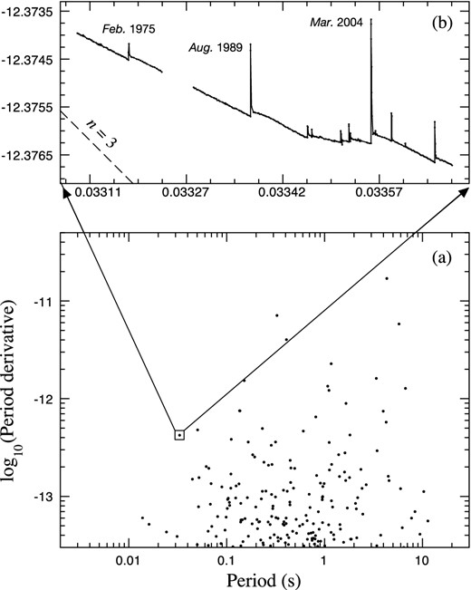
The progress of the Crab Pulsar across the |$P{\rm -}\dot{P}$| diagram. (a) The upper part of the standard |$P{\rm -}\dot{P}$| diagram and (b) an expanded view of the region containing the Crab pulsar, showing its motion during the past 45 years. The dashed line represents the path that would be followed by a pulsar having braking index n = 3.
7 CONCLUSIONS
The slowdown of the rotation rate of the Crab pulsar, including the effect of the glitches, could be described by a power law with braking index of around 2.34. The spin evolution is, however, affected by the steps in slowdown rate at glitches; removing these reveals an underlying simple slowdown with braking index 2.519(2). The average effect of the glitches is to increase the rate of slowdown by about 6 per cent. This description of the slowdown fails during an 11-yr period which coincides with a period of increased glitch activity.
Including the exponential component of the persistent step in slowdown rate at glitches allows an almost complete separation of the effects of glitches from the underlying slowdown. This component is in the form of an exponential with time constant 320 d, asymptotically reaching a value which nearly doubles the previously known effect.
The n = 2.5 braking index, lower than the conventional value n = 3 for a rotating magnetic dipole, may be attributed to a combination of a secular increase in magnetic inclination angle and a monopolar wind torque. If the rate of mass-loss in the wind persists, the braking index is expected to reduce towards n = 1, possibly accounting for the low index observed in the Vela pulsar.
The observed pattern of glitch activity, including the 11-yr period of increased glitch activity, does not agree well with the random behaviour expected from self-organized criticality.
Pulsar research at Jodrell Bank Centre for Astrophysics (JBCA) is supported by a consolidated grant from the UK Science and Technology Facilities Council (STFC). CME acknowledges the support from STFC and FONDECYT (postdoctorado 3130512).
