


ABSTRACT
The INT/WFC Photometric Hα Survey of the Northern Galactic Plane (IPHAS) is a 1800 deg2 imaging survey covering Galactic latitudes |b| < 5° and longitudes ℓ = 30°–215° in the r, i, and Hα filters using the Wide Field Camera (WFC) on the 2.5-m Isaac Newton Telescope (INT) in La Palma. We present the first quality-controlled and globally calibrated source catalogue derived from the survey, providing single-epoch photometry for 219 million unique sources across 92 per cent of the footprint. The observations were carried out between 2003 and 2012 at a median seeing of 1.1 arcsec (sampled at 0.33 arcsec pixel−1) and to a mean 5σ depth of 21.2 (r), 20.0 (i), and 20.3 (Hα) in the Vega magnitude system. We explain the data reduction and quality control procedures, describe and test the global re-calibration, and detail the construction of the new catalogue. We show that the new calibration is accurate to 0.03 mag (root mean square) and recommend a series of quality criteria to select accurate data from the catalogue. Finally, we demonstrate the ability of the catalogue's unique (r − Hα, r − i) diagram to (i) characterize stellar populations and extinction regimes towards different Galactic sightlines and (ii) select and quantify Hα emission-line objects. IPHAS is the first survey to offer comprehensive CCD photometry of point sources across the Galactic plane at visible wavelengths, providing the much-needed counterpart to recent infrared surveys.
1 INTRODUCTION
The INT/WFC Photometric Hα Survey of the Northern Galactic Plane (IPHAS; Drew et al. 2005) is providing new insights into the contents and structure of the disc of the Milky Way. This large-scale programme of observation – spanning a decade so far and using more than 300 nights in competitive open time at the Isaac Newton Telescope (INT) in La Palma – aims to provide the digital update to the photographic northern Hα surveys of the mid-20th century (see Kohoutek & Wehmeyer 1999). By increasing the sensitivity with respect to these preceding surveys by a factor of ∼1000 (7 mag), IPHAS can expand the limited bright samples of Galactic emission-line objects previously available into larger, deeper, and more statistically robust samples that will better inform our understanding of the early and late stages of stellar evolution. Since the publication of the Initial Data Release (IDR; González-Solares et al. 2008), these aims have begun to be realized through a range of published studies including a preliminary catalogue of candidate emission-line objects (Witham et al. 2008); discoveries of new symbiotic stars (Corradi et al. 2008, 2010, 2011; Rodríguez-Flores et al. 2014); new cataclysmic variables (Witham et al. 2007; Wesson et al. 2008; Aungwerojwit et al. 2012); new groups of young stellar objects (YSOs; Vink et al. 2008; Barentsen et al. 2011; Wright et al. 2012); new classical Be stars (Raddi et al. 2013); along with discoveries of new supernova remnants (Sabin et al. 2013), and new and remarkable planetary nebulae (Mampaso et al. 2006; Viironen et al. 2009a,b; Sabin et al. 2010, 2014; Corradi et al. 2011; Viironen et al. 2011).
Over the years it has become apparent that the legacy of IPHAS will reach beyond these traditional Hα applications of identifying emission-line stars and nebulae. Through the provision of r and i broad-band photometry alongside narrow-band Hα data, IPHAS has created the opportunity to study Galactic plane populations in a new way. For example, the survey's unique (r − Hα, r − i) colour–colour diagram has been shown to provide simultaneous constraints on intrinsic stellar colour and interstellar extinction (Drew et al. 2008). This has opened the door to a wide range of Galactic science applications, including the mapping of extinction across the plane in three dimensions and the probabilistic inference of stellar properties (Sale et al. 2009, 2010, 2014; Giammanco et al. 2011; Sale 2012; Barentsen et al. 2013). In effect, the availability of narrow-band Hα alongside r and i magnitudes provides coarse spectral information for huge samples of stars which are otherwise too faint or numerous to be targeted by spectroscopic surveys (cf. the use of Stromgren uvbyHβ photometry at blue wavelengths). For such science applications to succeed, however, it is vital that the imaging data are transformed into a homogeneously calibrated photometric catalogue, in which quality problems and duplicate detections are flagged.
When the previous release – the IDR – was created in late 2007, just over half of the survey footprint was covered and the data were insufficiently complete to support a homogeneously calibrated source catalogue. The goal of this paper is to present the next release, which supersedes the IDR by including a global re-calibration and by taking the coverage up to 92 per cent of the survey area. In this work, we (i) explain the data reduction and quality control procedures that were applied, (ii) describe and test the new photometric calibration, and (iii) detail the construction of the source catalogue and demonstrate its use.
In Section 2, we start by recapitulating the key points of the survey observing strategy. In Section 3, we describe the data reduction and quality control procedures. In Section 4, we explain the global re-calibration, in which we draw upon the AAVSO Photometric All-Sky Survey (APASS) and test our results against the Sloan Digital Sky Survey (SDSS). In Section 5, we explain how the source catalogue was compiled. In Section 6, we discuss the properties of the catalogue and in Section 7 we demonstrate the scientific exploitation of the colour/magnitude diagrams. Finally, in Section 8, we discuss access to the catalogue and an online library of reduced images. The paper ends with conclusions in Section 9 where we also outline our future ambitions.
2 OBSERVATIONS
The detailed properties of the IPHAS observing programme have been presented before by Drew et al. (2005) and González-Solares et al. (2008). To set the stage for this release, we recap some key points in this section (see Table 1 for a quick-reference overview). IPHAS is an imaging survey of the Galactic plane north of the celestial equator, from which photometry in Sloan r and i is extracted along with narrow-band Hα. It is carried out using the Wide Field Camera (WFC) on the 2.5-m INT in La Palma. It is the first digital survey to offer comprehensive optical CCD photometry of point sources in the Galactic plane; the footprint spans a box of roughly 180 by 10 deg, covering Galactic latitudes −5° < b < +5° and longitudes 30° < ℓ < 215°.
The WFC is a mosaic of four CCDs that captures a sky area of close to 0.29 deg2 at a pixel scale of 0.33 arcsec pixel−1. To cover the northern plane with some overlap, the survey area was divided into 7635 telescope pointings. Each of these pointings is accompanied by an offset position displaced by +5 arcmin in Dec. and +5 arcmin in RA, to deal with inter-CCD gaps, detector imperfections, and to enable quality checks. An example footprint of a pointing and its offset position is shown in Fig. 1. Hence, the basic unit of observation amounts to 2 × 3 exposures, in which each of the three survey filters is exposed at two offset sky positions within, typically, an elapsed time of 10 min. We shall refer to the unit of three exposures at the same position as a field, and the combination of two fields at a small offset as a field pair. Altogether, the survey contains 15 270 fields grouped into 7635 field pairs. To achieve the desired survey depth of 20th magnitude or fainter in each filter, the exposure times were set at 120 s (Hα), 30 s (r), and 10 s (i) in the vast majority of the survey observations.1
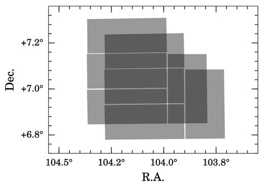
Example footprint of a pointing and its offset position. Each field in the survey is accompanied by an offset field at 5 arcmin west and south to deal with gaps between the CCDs. This unit of observation is called a field pair, which is observed in all three filters within a span of 10 min. The WFC is a mosaic of four CCDs, and hence a field pair is composed of eight CCD frames. In this example, each CCD is plotted as a semitransparent grey rectangle to highlight the overlap regions. Note that the L-shaped arrangement of the CCD mosaic allows nearly the entire field to be captured using just two pointings, apart from two ∼ 10-arcsec-wide squares which are located where inter-CCD gaps overlap.
Data-taking began in the second half of 2003, and every field had been observed at least once by the end of 2008. At that time, only 76 per cent of the field pairs satisfied our minimum quality criteria, however. The problems affecting the 24 per cent falling below survey standard were, most commonly, variable cloud cover; poor seeing; technical faults (the quality criteria will be detailed in the next section). Since then, a programme of repeat observations has been in place to improve data quality. As a result, 92 per cent of the survey footprint now benefits from quality-approved data. The most recent observations included in this release were obtained in 2012 November.
Fig. 2 shows the footprint of the quality-approved observations included in this work. The fields which remain missing – covering 8 per cent of the survey area – are predominantly located towards the Galactic anticentre at ℓ > 120°. Fields at these longitudes are mainly accessed from La Palma in the months of November and December, which is when the La Palma weather and seeing conditions are often poor, forcing many (unsuccessful) repeat observations. To enable the survey to be brought to completion, a decision was made recently to limit repeats in this area to individual fields requiring replacement, i.e. fresh observations in all three filters may only be obtained at one of the two offset positions. The catalogue is structured such that it is clear where contemporaneous observations of both halves of a field pair are available.

Survey area showing the footprints of all the quality-approved IPHAS fields which have been included in this data release. The area covered by each field has been coloured black with a semitransparent opacity of 20 per cent such that regions where fields overlap are darker. The IPHAS strategy is to observe each field twice with a small offset, and hence the vast majority of the area is covered twice (dominant grey colour). There are small overlaps between all the neighbouring fields which can be seen as a honeycomb pattern of dark grey lines across the survey area. Regions with incomplete data are apparent as white gaps (no data) or in light grey (indicating that one offset is missing). The dark vertical strip near ℓ ≃ 125° is an arbitrary consequence of the tiling pattern, which was populated starting from 0 h in right ascension.
3 DATA REDUCTION AND QUALITY CONTROL
3.1 Initial pipeline processing
All raw IPHAS data were transferred to the Cambridge Astronomical Survey Unit (CASU) for initial processing and archiving. The procedures used by CASU were originally devised for the INT Wide Field imaging Survey (WFS; McMahon et al. 2001; Irwin et al. 2005), which was a 200 deg2 extragalactic survey programme carried out between 1998 and 2003. Because IPHAS uses the same telescope and camera combination, we have been able to benefit from the existing WFS pipeline. A description of the processing steps can be found in Irwin & Lewis (2001). Its application to IPHAS has previously been described by Drew et al. (2005) and González-Solares et al. (2008), and some elements of the source code are available online.2 In brief, the imaging processing part of the pipeline takes care of bias subtraction, the linearity correction, flat-fielding with internal gain correction, and de-fringing for the i band.
Object detection and parametrization is then carried out using the standard methods developed by CASU, which can be summarized in four steps (a discussion on each of these steps and related points can be found in Irwin 1985, 1997) as follows.
The local sky background is estimated by first computing an iteratively sigma-clipped median intensity on a grid of 64 × 64 pixel bins across the image from each detector. This is usually robust against contaminating sources corrupting the background level. The resulting array of background values is then filtered to further reduce the effect of large objects on the local background level. Bilinear interpolation is then used to obtain an estimate of the background level at the original image pixel scale.
To improve faint object detection, each image is smoothed with a matched detection filter which is used in conjunction with the unsmoothed image for object detection and parametrization.
Objects, or blends of objects, are detected by identifying groups of four or more neighbouring contiguous pixels in which the intensity exceeds the background level by at least 1.25σ on the matched filtered image. Objects are deblended using a sequence of successively higher detection levels.
The objects are parametrized using the unsmoothed image at these pixel locations: positions are obtained based on an intensity-weighted isophotal centre-of-gravity of each object; whilst photometry is derived by measuring the intensity in a series of soft-edged circular apertures covering a range of diameters (1.2, 2.3, 3.3, 4.6, 6.6, and 9.2 arcsec). Objects are also classified morphologically – stellar, extended, or noise – based on their intensity as a function of aperture size and on their intensity-weighted second moments, where the latter are used to derive an estimate of object ellipticity.
The parametrization of overlapping objects is refined by simultaneous fitting of soft-edged apertures to each blend, effectively carrying out ‘top hat’ profile fitting where it is necessary. We note that the parametrization of these blended objects is naturally less reliable than that of single, unconfused sources, which is why they are flagged in the catalogue (to be explained in Section 5).
Having carried out object detection, the astrometric calibration is then determined. The solution starts with a rough World Coordinate System based on the known telescope and camera geometry, using a Zenithal Polynomial projection (Calabretta & Greisen 2002) to model the (fixed) field distortion of the camera. The parameters of this solution are then progressively refined by fitting against the Two Micron All Sky Survey (2MASS; Skrutskie et al. 2006), albeit without correcting for the ∼10 yr of proper motion between the IPHAS and 2MASS epochs. The resulting fit has previously been shown to deliver results which are internally consistent to better than 0.1 arcsec across the detector array (González-Solares et al. 2008).
An external validation of the astrometry has been carried out by comparing our positions against the United States Naval Observatory CCD Astrograph Catalog (UCAC4; Zacharias et al. 2013). Fig. 3 shows the distribution of the astrometric offsets computed for 1.3 million stars in the magnitude range 13 < r < 15, which is the range where both surveys overlap and where the formal mean error of UCAC4 is better than 50 mas (Zacharias et al. 2010). We find the mean difference in position between IPHAS and UCAC4 to be 94 mas, which is satisfactory for our purposes. The remaining residuals are in part due to the motion of the Earth through our Galaxy, which we did not account for.
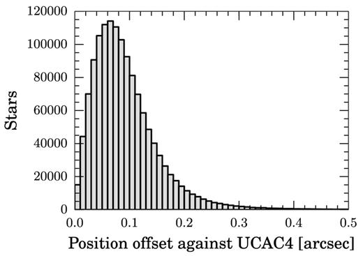
Distribution of the astrometric residuals of stars which appear both in IPHAS DR2 and UCAC4 within a cross-matching distance of 1 arcsec. The residuals were computed for the 1.3 million stars in the IPHAS catalogue which are not blended, not saturated, and fall in the magnitude range 13 < r < 15. The mean and standard deviation of this distribution equal 94 ± 65 mas.
At the time of preparing Data Release 2 (DR2), the pipeline had processed 74 195 single-band IPHAS exposures in which a total of 1.9 billion candidate detections were made. This total inevitably includes spurious objects, artefacts, and duplicate detections; in Section 5, we will explain how these have been removed or flagged in the final catalogue.
The entire data set – comprising 2.5 terabyte of FITS files – was then transferred to the University of Hertfordshire for the purpose of transforming the raw detection tables into a source catalogue which (i) is quality controlled, (ii) is homogeneously calibrated, and (iii) contains user-friendly columns and warning flags. It is these post-processing steps which distinguish this release from the IDR, which (i) enforced less stringent quality limits, (ii) did not offer a global calibration, and (iii) provided a catalogue in which duplicate detections of unique sources were not flagged. These improvements are explained next.
3.2 Quality control
Observing time for IPHAS is obtained on a semester-by-semester basis through the open time allocation committees of the Isaac Newton Group (ING) of telescopes. The survey is allocated specific observing dates rather than particular observing conditions. In consequence, data were acquired under a large range of atmospheric conditions. Data taken under unsuitable conditions have been rejected using seven quality criteria, which ensure a good and homogeneous level of quality across the data release.
Depth. We discarded any exposures for which the 5σ limiting magnitude3 was brighter than 20th magnitude in the r band or brighter than 19th in i or Hα. Such data were typically obtained during poor weather or full Moon. Most observations were significantly better than these limits. Fig. 4 presents the distribution of limiting magnitudes for all quality-approved fields; the mean depths and standard deviations are 21.2 ± 0.5 (r), 20.0 ± 0.3 (i), and 20.3 ± 0.3 (Hα). The depth achieved depended most strongly on the presence of the Moon, which was above the horizon during 62 per cent of the observations. The great range in sky brightness this produced is behind the wide and bi-modal shape of the r-band limiting magnitude distribution (top panel in Fig. 4). In contrast, the depths attained in i and Hα are less sensitive to moonlight, leading to narrower magnitude limit distributions (middle and bottom panels in Fig. 4). To a lesser extent, the wide spread in the r-band depth is also explained by the shorter exposure time that was used for this band during the first months of data-taking.
Ellipticity. The ellipticity of a point source, defined as e = 1 − b/a with b the semiminor and a the semimajor axis, is a morphological measure of the elongation of the point spread function (PSF). It is expected to be zero (circular) in a perfect noise-free imaging system, but it is slightly non-zero in any real telescope data due to optical distortions, tracking errors, and photon plus readout noise. Indeed, it is worth noting that IPHAS data have been collected from unguided exposures that rely entirely on the INT's tracking capability. The mean ellipticity measured in the data is 0.09 ± 0.04. There have been sporadic episodes with higher ellipticities due to mechanical glitches in the telescope tracking system. As a result, 3 per cent of our images show an average ellipticity across the detectors which is worse than e > 0.2. The inspection of these examples revealed no evidence for degraded photometry up to ellipticities of 0.3. We have excluded a small number of exposures which exceeded e = 0.3.
Seeing. The original survey goal was to obtain data at a resolution better than 1.7 arcsec, as evaluated by measuring the average PSF full width at half-maximum (FWHM) across the detectors. This target is currently attained across 86 per cent of the footprint. To increase the sky area offered by the data release slightly, we have decided to accept data obtained with FWHM up to 2.5 arcsec. Fig. 5 presents the distribution of the PSF FWHM for the approved fields. In the r band, 90 per cent is better than 1.5 arcsec, 50 per cent is better than 1.1 arcsec, and 10 per cent is better than 0.8 arcsec. In Section 5, we will explain that the photometry compiled in the source catalogue is normally derived from the field with the best-available seeing for a given object, and that the FWHM measurement is available as a column in the catalogue.
Photometric repeatability. The IPHAS field-pair observing strategy normally ensures that every pointing is immediately followed by an offset pointing at a displacement of +5 arcmin in Dec. and +5 arcmin in RA. This allows pairs of images to be checked for the presence of clouds or electronic noise. To exploit this information, the overlap regions of all field pairs were systematically cross-matched to verify the consistency of the photometry for stars observed in both pointings. We automatically rejected field pairs in which more than 2 per cent of the stars showed an inconsistent measurement at the level of 0.2 mag, or more than 25 per cent were inconsistent at the level of 0.1 mag. These limits were set empirically after inspecting the images and photometry by eye.
Visual examination. Images, colour mosaics, and the associated photometric colour/magnitude diagrams were inspected by a team of 20 survey members, such that each image in the data release was looked at by at least three different pairs of eyes. Images affected by clouds or extreme levels of scattered moonlight were flagged, investigated, and excluded from the release if deemed necessary.
Source density mapping. Spatial maps showing the number density of the detected sources down to 20th magnitude were created to verify the health of the data and to check for unexpected artefacts. In particular, we created density maps which showed the number of unique sources obtained by cross-matching the detection tables of all three bands with a maximum matching distance of 1 arcsec. This was effective for revealing fields with an inaccurate astrometric solution in one of the bands, which were subsequently corrected.
Contemporaneous field data. Finally, only exposures which are part of a sequence of three consecutive images of the same field (Hα, r, i) were considered for inclusion in the release. This ensures that the three bands for a given field are observed contemporaneously – nearly always within 5 min of each other. We note that the source catalogue details the exact epoch at the start of each exposure (columns rMJD, iMJD, haMJD).
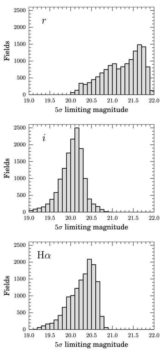
Distribution of the 5σ limiting magnitude across all quality-approved survey fields for r (top), i (middle), and Hα (bottom). Fields with a limiting magnitude brighter than 20th (r) or 19th (Hα, i) were rejected from the data release. The r-band depth is most sensitive to the presence of the Moon above the horizon: this is the main reason for the wide, bi-modal character of its distribution.
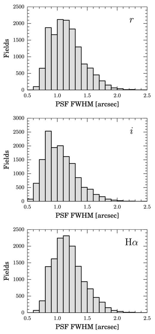
Distribution of the PSF FWHM for all the quality-approved fields included in the release, measured in r (top), i (middle), and Hα (bottom). The PSF FWHM measures the effective image resolution that arises from the combination of atmospheric and dome seeing.
The above criteria were satisfied by at least one observing attempt for 14 115 out of the 15 270 planned fields (92 per cent). In some cases, more than one successful attempt to observe a field was available due to stricter quality criteria being applied in the initial years of the survey. In such cases, only the attempt with the best seeing and depth has been selected for inclusion in the catalogue, in order to deliver the most accurate measurement at a single epoch.
We note that some of the excluded data may nevertheless be useful for e.g. time-domain studies of bright stars. The discarded data are available through our website, but will be ignored in the remainder of this work.
4 PHOTOMETRIC CALIBRATION
Having obtained a quality-approved set of observations, we now turn to the challenge of placing the data on to a uniform photometric scale.
4.1 Provisional nightly calibration
The broad-band ZP were determined such that the resulting magnitude system refers to the spectral energy distribution (SED) of Vega as the zero-colour object. Colour equations were used to transform between the IPHAS passbands and the Johnson–Cousins system of the published standard-star photometry. The entire procedure has been found to deliver ZP which are accurate at the level of 1–2 per cent in stable photometric conditions (González-Solares et al. 2011).
Key properties of IPHAS DR2.
| Property | Value |
|---|---|
| Telescope | 2.5-m INT |
| Instrument | Wide Field Camera (WFC) |
| Detectors | Four 2048 × 4100 pixel CCDs |
| Pixel scale | 0.33 arcsec pixel−1 |
| Filters | r, i, Hα |
| Filter properties | See Table 2 |
| Magnitude system | Vega |
| Exposure times | 30 s (r), 10 s (i), 120 s (Hα) |
| Saturation limit | 13 (r), 12 (i), 12.5 (Hα) |
| Detection limit (5σ, mean) | 21.2 (r), 20.0 (i), 20.3 (Hα) |
| PSF FWHM (median) | 1.1 arcsec (r), 1.0 arcsec (i), 1.1 arcsec (Hα) |
| Survey area | ∼1860 deg2 |
| Footprint boundaries | −5° < b < +5°, 29° < ℓ < 215° |
| Observing period | 2003 August–2012 November |
| Website | www.iphas.org |
Mean monochromatic flux of Vega in the IPHAS filter system, defined as 〈fλ〉 = ∫fλ(λ)S(λ)λdλ/∫S(λ)λdλ, where S(λ) is the photon response function (which includes atmospheric transmission, filter transmission, and CCD response) and fλ(λ) is the CALSPEC SED for Vega (Bohlin 2014). For reference, we also provide the filter equivalent width EW = ∫S(λ)dλ, the mean photon wavelength λ0 = ∫S(λ)λdλ/∫S(λ)dλ, and the pivot wavelength |$\lambda _{\rm p} = \sqrt{\int\! {S(\lambda )\lambda {\rm d}\lambda } / \!\!\int {\frac{S(\lambda )}{\lambda } {\rm d}\lambda }}$|. These notations follow the definitions by Bessell & Murphy (2012). After multiplying 〈fλ〉 by the EW, we find that the detected flux for Vega in Hα is 3.14 mag less than that received in r.
| Filter | 〈fλ〉 | EW | λ0 | λp |
|---|---|---|---|---|
| (erg cm−2 s−1 Å−1) | (Å) | (Å) | (Å) | |
| r | 2.47 × 10⁻⁹ | 785.6 | 6223 | 6211 |
| Hα | 1.81 × 10⁻⁹ | 59.6 | 6568 | 6568 |
| i | 1.30 × 10⁻⁹ | 759.9 | 7674 | 7661 |
| Filter | 〈fλ〉 | EW | λ0 | λp |
|---|---|---|---|---|
| (erg cm−2 s−1 Å−1) | (Å) | (Å) | (Å) | |
| r | 2.47 × 10⁻⁹ | 785.6 | 6223 | 6211 |
| Hα | 1.81 × 10⁻⁹ | 59.6 | 6568 | 6568 |
| i | 1.30 × 10⁻⁹ | 759.9 | 7674 | 7661 |
4.2 Global re-calibration
Despite the best efforts made to obtain a nightly calibration, large surveys naturally possess field-to-field variations due to atmospheric changes during the night and imperfections in the pipeline or the instrument (e.g. the WFC is known to suffer from sporadic errors in the timing of exposures). This is demonstrated in Fig. 6(a), where we show the combined colour–colour diagram for nearly 3000 fields across an area of 400 deg2. The main locus of stars is poorly defined in the diagram due to the presence of incorrectly calibrated fields, which need to be corrected during a global re-calibration step. The application of such a procedure, to be explained below, has revealed that the error in our initial nightly calibration exceeded 0.1 mag in 12 per cent of the fields, and even exceeded 0.5 mag in 0.7 per cent. Fig. 6(b) demonstrates the improvement in the colour–colour diagram after re-calibrating.
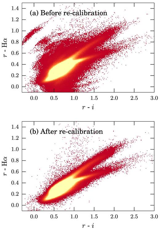
IPHAS (r − Hα, r − i) colour–colour diagram covering an area of 400 deg2, shown before (panel a) and after (panel b) re-calibration. Both figures were created by combining the stars detected across all 2801 quality-approved fields which are located towards the Galactic anticentre (160° < ℓ < 200°). The diagrams are plotted as 2D histograms which show the density of sources in bins of 0.01-by-0.01 mag; bins containing 1–200 sources are coloured red, while bins containing more than 400 sources are bright yellow. The diagrams include all stars brighter than r < 18 which were classified by the pipeline as ‘a10point’ (indicating a high-significance point source detection with accurate photometry in all bands, to be explained in Section 6.2). The objects which are seen to fall above the locus of stars after re-calibration are likely to be genuine Hα emission-line objects.
Notable past examples of surveys which required global re-calibration include 2MASS (Nikolaev et al. 2000), SDSS (Padmanabhan et al. 2008) and the Panoramic Survey Telescope And Rapid Response System survey (Pan-STARRS; Schlafly et al. 2012), which all achieved photometry that is globally consistent to within 0.01–0.02 mag after re-calibration.
Surveys which observe identical stars at different epochs can use the repeat measurements to ensure a homogeneous calibration. For example, 2MASS attained its global calibration by observing two standard fields each hour, allowing ZP variations to be tracked over short time-scales (Nikolaev et al. 2000). Alternatively, the SDSS and PanSTARRS surveys could benefit from revisiting regions in their footprint to carry out a so-called ubercalibration5 procedure, in which repeat measurements of stars in different nights are used to fit the calibration parameters (Ivezić et al. 2007; Padmanabhan et al. 2008; Schlafly et al. 2012).
Unfortunately, these schemes cannot be applied directly to IPHAS for two reasons. First, the survey was carried out in competitively allocated observing time on a common-user telescope, rendering the 2MASS approach of observing standards at a high frequency prohibitively expensive (it does not help that standard fields are very scarce within the Galactic plane). Secondly, IPHAS is not specified as a variability survey, with the result that stars are not normally observed at more than one epoch, unless they happen to fall within a narrow overlap region between two neighbouring field pairs.
We have found the information contained in our narrow overlap regions to be insufficient to constrain the calibration parameters well enough. This is because photometry at the extreme edges of the WFC – where neighbouring field pairs overlap – is prone to systematics at the level of 1–2 per cent. The cause of these errors is thought to include the use of twilight sky flats in the pipeline, which are known to be imperfect for calibrating stellar photometry due to stray light and vignetting (e.g. Manfroid 1995). Moreover, the illumination correction in the overlap regions is more affected by a radial geometric distortion in the WFC, which causes the pixel scale to increase as the edges are approached (González-Solares et al. 2011). Although these systematics are reasonably small within a single field, they can accumulate during a re-calibration process, causing artificial ZP gradients across the survey unless controlled by other external constraints.
For these reasons, we have not depended on an ubercalibration-type scheme alone, but have opted to involve an external reference survey – where available – to bring the majority of our data on to a homogeneous calibration.
4.2.1 Correcting ZP using APASS
We have been able to benefit from APASS (http://www.aavso.org/apass) to bring most of the survey on to a uniform scale. Since 2009, APASS has been using two 20-cm-astrographs to survey the entire sky down to ∼17th magnitude in five filters which include Sloan r and i (Henden et al. 2012). The most recent catalogue available at the time of preparing this work was APASS DR7, which provides a good coverage across ∼half of the IPHAS footprint. The overlap regions are shown in Fig. 7. The photometric accuracy of APASS is currently estimated to be at the level of 3 per cent, which is significantly better than the original nightly calibrations of IPHAS which are only accurate to ∼10 per cent when compared to APASS (Table 3). APASS achieves its uniform accuracy by measuring each star at least two times in photometric conditions, along with ample standard fields, benefiting from the large 3-by-3 deg field of view of its detectors.
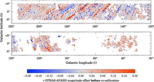
Median magnitude offset in the r band between IPHAS and APASS, plotted on a field-by-field basis prior to the re-calibration procedure. Each square represents the footprint of an IPHAS field which contains at least 30 stars with a counterpart in the APASS DR7 catalogue. The colours denote the median IPHAS−APASS magnitude offset in each field, which was computed after applying the APASS-to-IPHAS transformation to the APASS magnitudes (equation 3). For clarity, we do not show the fields at the offset positions.
Magnitude offsets for objects cross-matched between IPHAS and APASS/SDSS before the global re-calibration was carried out. We characterize the distribution of the offsets, which is approximately Gaussian in each case, by listing the mean and the standard deviation values. We remind the reader that transformations were applied to the APASS and SDSS magnitudes to bring them into the Vega-based IPHAS system prior to computing the offsets.
| Before re-calibration | Mean | σ |
|---|---|---|
| r (IPHAS−APASS) | +0.014 | 0.104 |
| i (IPHAS−APASS) | +0.007 | 0.108 |
| r (IPHAS−SDSS) | +0.016 | 0.088 |
| i (IPHAS−SDSS) | +0.010 | 0.089 |
| Before re-calibration | Mean | σ |
|---|---|---|
| r (IPHAS−APASS) | +0.014 | 0.104 |
| i (IPHAS−APASS) | +0.007 | 0.108 |
| r (IPHAS−SDSS) | +0.016 | 0.088 |
| i (IPHAS−SDSS) | +0.010 | 0.089 |
With the aim of bringing IPHAS to a similar accuracy of 3 per cent, we used the APASS catalogue to identify and adjust the calibration of all IPHAS fields which showed a magnitude offset larger than 0.03 mag against APASS. Experience of re-running the calibration and testing the results showed us that it was inadvisable to tune more finely the match for IPHAS data obtained in what were generally the most photometric nights. To this end, the r- and i-band detection tables of each IPHAS field were cross-matched against the APASS DR7 catalogue using a maximum matching distance of 1 arcsec. The magnitude range was limited to 13 < rAPASS < 16.5 and 12.5 < iAPASS < 16.0 in order to avoid sources brighter than the IPHAS saturation limit on one hand, and to avoid sources near the faint detection limit of APASS on the other.
Having transformed APASS magnitudes into the IPHAS system, we then computed the median magnitude offset for each field which contained at least 30 cross-matched stars. This was achieved for 48 per cent of our fields (shown in Figs 7 and 8). The offsets follow a near-Gaussian distribution with mean and sigma 0.014 ± 0.104 mag in r and 0.007 ± 0.108 mag in i (Table 3). A total of 4596 IPHAS fields showed a median offset exceeding ±0.03 mag in either r or i when compared to APASS.
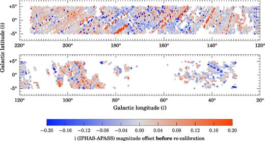
Same as Fig. 7 for the i band.
We then applied the most important step in our re-calibration scheme, which is to adjust the provisional ZP of these 4596 aberrant fields such that their offset is brought to zero. This allowed the mean IPHAS-to-APASS offset to be brought down to 0.000 ± 0.011 mag in both r and i (Table 4). The procedure of fitting magnitude transformations and correcting the IPHAS ZP was repeated a few times to ensure convergence, which was closely approached after the first iteration.
Same as Table 3, but computed after the global re-calibration was carried out. The mean and standard deviation values of the offsets have improved significantly.
| After re-calibration | Mean | σ |
|---|---|---|
| r (IPHAS−APASS) | +0.000 | 0.011 |
| i (IPHAS−APASS) | +0.000 | 0.011 |
| r (IPHAS−SDSS) | −0.001 | 0.029 |
| i (IPHAS−SDSS) | −0.002 | 0.032 |
| After re-calibration | Mean | σ |
|---|---|---|
| r (IPHAS−APASS) | +0.000 | 0.011 |
| i (IPHAS−APASS) | +0.000 | 0.011 |
| r (IPHAS−SDSS) | −0.001 | 0.029 |
| i (IPHAS−SDSS) | −0.002 | 0.032 |
4.2.2 Adjusting fields not covered by APASS
At the time of writing, the APASS catalogue did not provide sufficient coverage for 7359 of our fields. Fortunately, these fields are located mainly at low Galactic longitudes (cf. Figs 7 and 8), which were typically observed during the summer months when photometric conditions are more prevalent at the telescope. These remaining fields have nevertheless been brought on to the same uniform scale by employing an ubercalibration-style scheme, which minimizes the magnitude offsets between stars located in the overlap regions between neighbouring fields.
An algorithm for achieving this minimization has previously been described by Glazebrook et al. (1994). In brief, there are two fundamental quantities to be minimized between each pair of overlapping exposures, denoted by the indices i and j. First, the mean magnitude difference between stars in the overlap region Δij = 〈mi − mj〉 = −Δji is a local constraint. Secondly, to ensure that the solution does not stray far from the existing calibration, the difference in ZP ΔZPij = −ΔZPji between each pair of exposures must also be minimized.
We enforce a strong external constraint on the solution by keeping the ZP fixed for the fields which have already been compared and calibrated against APASS. We hereafter refer to these fields as anchors. It is asserted that the ZP ai of the anchor fields are known and not solved for. However, they do appear in the vector bj as constraints. In addition to the APASS-based anchors, we selected 3273 additional anchor fields by hand to provide additional constraints in regions not covered by APASS. These extra anchors were deemed to have accurate ZP based on (i) the information contained in the observing logs, (ii) the stability of the standard-star ZP during the night, and (iii) photometricity statistics provided by the Carlsberg Meridian Telescope, which is located ∼500 m from the INT.
We then solved equation (6) for the r and i bands separately using the least-squares routine in python's scipy.sparse module for sparse matrix algebra. This provided us with corrected ZP for the remaining fields, which were shifted on average by +0.02 ± 0.11 in r and +0.01 ± 0.12 in i compared to their provisional calibration.
We then turned to the global calibration of the Hα data. It is not possible to re-calibrate the narrow-band in the same way as the broad-bands, because the APASS survey does not offer Hα photometry. We can reasonably assume, however, that the corrections required for r and Hα are identical, much of the time, because the IPHAS data-taking pattern ensured that a field's Hα and r-band exposures were taken consecutively, albeit separated by an ∼30 s read-out time. Hence, we have corrected the Hα ZP by re-using the ZP adjustments that were derived for the r band in the earlier steps. An exception was made for 3101 fields for which our quality control routines revealed strong ZP variations during the night, suggesting non-photometric conditions. In these cases, the Hα ZP were adjusted by solving equation (6) rather than by simply applying equation (2).
4.3 Testing the calibration against SDSS
Having re-calibrated all fields to the expected APASS accuracy of 3 per cent, we turned to a different survey, SDSS DR9 (Ahn et al. 2012), to validate the results. SDSS DR9 includes photometry across several strips at low Galactic latitudes, which were observed as part of the Sloan Extension for Galactic Understanding and Exploration (Yanny et al. 2009). These strips provide data across 18 per cent of the fields in our data release. We cross-matched the IPHAS fields against the subset of objects marked as reliable stars in the SDSS catalogue6 in much the same way as for APASS, with the difference of selecting from the fainter magnitude ranges of 15 < rSDSS < 18.0 and 14.5 < iSDSS < 17.5. This provided us with a set of 1.2 million cross-matched stars.
These global transformations were deemed adequate for the purpose of validating our calibration in a statistical sense. Separate equations were derived towards different sightlines to investigate the effects of varying reddening regimes. The colour term was found to show some variation towards weakly reddened areas, where different stellar populations are observed. The vast majority of red objects in the global sample are those in highly reddened areas, however, which agree well with the global transformations and dominate the statistical appraisal of our calibration.
Having transformed SDSS magnitudes into the IPHAS system, we then computed the median magnitude offset for each IPHAS field which contained at least 30 objects with a cross-matched counterpart in SDSS. This was the case for 2602 fields. The median offsets for each of these fields are shown in Figs 9 and 10. Importantly, the mean offset and standard deviation found is −0.001 ± 0.029 mag in r and −0.002 ± 0.032 mag in i (Table 4). In comparison, offsets computed in the identical way before carrying out the re-calibration showed means of +0.016 ± 0.088 mag in r and +0.010 ± 0.089 mag in i (Table 4). We conclude that our re-calibration procedure has been successful in improving the uniformity of the calibration by a factor of 3 (i.e. from σ = 0.088 to 0.029 in r), and as such has achieved our aim of bringing the accuracy to the aimed level of 0.03 mag.

Median magnitude offset between IPHAS and SDSS in the r band after the re-calibration procedure using APASS was applied. Each square represents the footprint of an IPHAS field which contains at least 30 stars with a counterpart in the SDSS DR9 catalogue. The colours denote the median IPHAS−SDSS magnitude offset in each field, which was computed after applying the SDSS-to-IPHAS transformation to the SDSS magnitudes (equation 9).
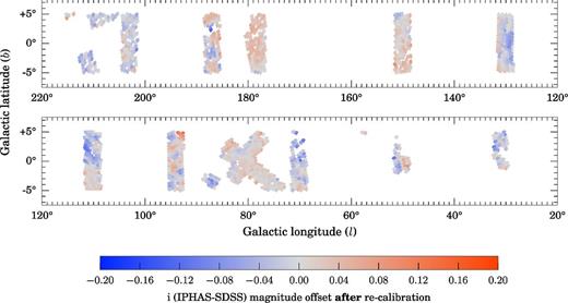
Same as Fig. 9 for the i band.
The SDSS comparison revealed a number of fields where the offsets exceeded 0.05 mag (523 fields) or even 0.1 mag (18 fields). This pattern of outliers is consistent with the tails of a Gaussian distribution with σ = 0.03. Furthermore, it should not be forgotten that both the SDSS and APASS calibrations are approximations to perfection and will not be entirely free of anomalies. Indeed, as we worked, we noticed the occasional unsurprising examples of inconsistency between these two surveys.
5 SOURCE CATALOGUE GENERATION
Having obtained a quality-checked and re-calibrated data set, we now turn to the challenge of transforming the observations into a user-friendly catalogue. The aim is to present the best-available information for each unique source in a convenient format, including flags to warn about quality issues such as source blending and saturation. Compiling the catalogue involved four steps:
the single-band detection tables produced by the CASU pipeline were augmented with new columns and warning flags;
the detection tables were merged into multiband field catalogues;
the overlap regions of the field catalogues were cross-matched to flag duplicate (repeat) detections and identify the primary (best) detection of each unique source; and
these primary detections were compiled into the final source catalogue.
Each of these four steps are explained next.
5.1 User-friendly columns and warning flags
Enhancement of the detection tables by creating new columns is the necessary first step because the tables generated by the CASU pipeline refer to source positions in pixel coordinates, to photometric measures in number counts, and so on, rather than in common astronomical units. To transform these data into user-friendly quantities, we have largely adopted the units and naming conventions which are in use at the Wide Field Camera (WFCAM) Science Archive (WSA; Hambly et al. 2008) and the Visible and Infrared Survey Telescope for Astronomy (VISTA) Science Archive (VSA; Cross et al. 2012). These archives curate the high-resolution near-infrared photometry from both the United Kingdom Infrared Telescope (UKIRT) Infrared Deep Sky Survey (UKIDSS; Lawrence et al. 2007) and the VISTA Variables in the Via Lactea survey (Minniti et al. 2010). There is a significant degree of overlap between the footprints of UKIDSS Galactic Plane Survey (GPS; Lucas et al. 2008) and IPHAS, and hence by adopting a similar catalogue format we hope to facilitate scientific applications which combine both data sets.
A detailed description of each column in our source catalogue is given in Appendix A. In the remainder of this section, we highlight the main features.
First, we note that each source is uniquely identified by an IAU-style designation of the form ‘IPHAS2 JHHMMSS.ss+DDMMSS.s’ (cf. column name in Appendix A), where ‘IPHAS2’ refers to the present data release and the remainder of the string denotes the J2000 coordinates in sexagesimal format. For convenience, the coordinates are also included in decimal degrees (columns ra and dec) and in Galactic coordinates (columns l and b). We have also included an internal object identifier string of the form ‘#run-#ccd-#detection’ (e.g. ‘64738-3-6473’), which documents the INT exposure number (#run), the CCD number (#ccd), and the row number in the CASU detection table (#detection). These columns are named rDetectionID, iDetectionID, haDetectionID.
Photometry is provided based on the 2.3-arcsec-diameter circular aperture by default (columns r, i, ha). The choice of this aperture size as the default is based on a trade-off between concerns about small number statistics and centroiding errors for small apertures on one hand, and diminishing signal-to-noise ratios (S/N) and source confusion for large apertures on the other hand. The user is not restricted to this choice, because the catalogue also provides magnitudes using three alternatives: the peak pixel height (columns rPeakMag, iPeakMag, haPeakMag), the circular 1.2-arcsec-diameter aperture (rAperMag1, iAperMag1, haAperMag1), and the 3.3-arcsec-diameter aperture (rAperMag3, iAperMag3, haAperMag3).
Each of these magnitude measurements have been corrected for the flux lost outside of the respective apertures, using a correction term which is inferred from the mean shape of the PSF measured locally in the CCD frame. In the case of a point source, the four alternative magnitudes are expected to be consistent with each other to within the photon noise uncertainty (which is given in columns rErr, rPeakMagErr, rAperMag1Err, rAperMag3Err, etc.). When this is not the case, it is likely that the source is either an extended object for which the aperture correction is invalid, or that the object has been incorrectly measured as a result of source blending or a rapidly spatially varying nebulous background. In Section 6.2, we will explain that the consistency of the different-aperture-magnitude measurements can be used as a criterion for selecting stellar objects with accurate photometry.
The brightness of each object as a function of increasing aperture size is also used by the CASU pipeline to provide a discrete star/galaxy7/noise classification flag (rClass, iClass, haClass) and a continuous stellarness-of-profile statistic (rClassStat, iClassStat, haClassStat). For convenience, we have combined these single-band morphological measures into band-merged class probabilities and flags using the merging scheme in use at the WSA8 (pStar, pGalaxy, pNoise, mergedClass, mergedClassStat).
Information on the quality of each detection is included in a series of additional columns. We draw attention to three useful flags which warn about the likely presence of a systematic error:
The saturated column is used to flag sources for which the peak pixel height exceeds 55 000 counts, which is typically the case for stars brighter than 12–13th magnitude in r. Although the pipeline attempts to extrapolate the brightness of saturated stars based on the shape of the PSF, such extrapolation is prone to error, and should be viewed as indicative rather than as precise measurement (systematic uncertainties as a function of magnitude will be discussed in Section 6.4).
The deblend column is used to flag sources which partially overlap with a nearby neighbour. Although the pipeline applies a deblending procedure to such objects, the procedure is currently applied separately in each band, and hence the (r − i) and (r − Hα) colours may be inaccurate if the deblending proceeded differently in each band.
The brightNeighb column is used to flag sources which are located within a radius of 5 arcmin from an object brighter than V = 7 according to the Bright Star Catalogue (Hoffleit & Jaschek 1991), or within 10 arcmin if the neighbour is brighter than V = 4. These brightest stars are known to cause systematic errors and spurious detections as a result of stray light and diffraction spikes.
In addition to the above, we also created warning flags for internal bookkeeping. For example, we flagged detections which fell in the strongly vignetted regions of the focal plane, which were truncated by CCD edges, or which were otherwise affected by bad pixels in the detector. No such detections have had to be included in the catalogue, as alternative detections were available in essentially all these situations, thanks to the IPHAS field-pair strategy. Hence, there has been no need to include these internal warning flags in the published source catalogue.
Finally, we note that basic information on the observing conditions is included (fieldID, fieldGrade, night, seeing). A table containing more detailed quality control information, indexed by fieldID, is made available on our website.
5.2 Band-merging the detection tables
The second step in compiling the source catalogue is to merge the contemporaneous trios of r, i, Hα detection tables into multiband field catalogues. This required a position matching procedure to link sources between the three bands. We used the TMATCHN function of the stilts software for this purpose, which allows rows from multiple tables to be matched (Taylor 2006). In brief, the algorithm identifies groups of linked detections such that (i) each detection is located within a specified maximum distance from one or more members of the group, (ii) each detection appears in exactly one group, and (iii) the largest possible groups are preferred (i.e. preferably containing three detections from all three bands). The result of the procedure is a band-merged catalogue in which each row corresponds to a group of linked r, i, and Hα detections which satisfy the matching distance criterion in a pair-wise sense. Sources for which no counterpart was identified in all three bands are retained in the catalogue as single- or double-band detections, with empty columns for the missing bands.
We employed a maximum matching distance of 1 arcsec, trading off completeness against reliability. On the one hand, a matching distance larger than 1 arcsec was found to allow too many spurious and unrelated sources to be linked. On the other, a value smaller than 1 arcsec would pose problems for very faint sources with large centroiding errors, and would occasionally fail near CCD corners, where the astrometric solution can show local systematic errors which exceed 0.5 arcsec. The position offsets between the r detection and detections in i, and/or Hα have been included in the catalogue, giving the user the option to tighten them further if necessary (columns iXi, iEta, haXi, haEta), or simply to examine light centre differences. We note that UKIDSS/GPS adopted the same maximum matching distance for similar reasons (Hambly et al. 2008).
The resulting band-merged catalogues were inspected by eye as part of our quality control procedures and were found to be reliable for the vast majority of objects. We do warn that blended objects can occasionally fall victim to source confusion during the band-merging procedure, which is a complicated problem that we have not attempted to resolve in this release. It is important to bear this in mind when appraising stars of seemingly unusual colours (such as candidate emission-line stars). If blending is flagged, or if the interband matching distance is unusually large, then the probability that the unusual colour is spurious due to source confusion is greatly increased.
5.3 Selecting the primary detections
We explained earlier that the survey contains repeat observations of identical sources as a result of field offsetting and overlaps. Amongst all sources in the magnitude range 13 < r < 19, we find that 65 per cent were detected twice and 25 per cent were detected three times or more. Only 9 per cent were detected once.
Since the principal aim of this data release is to provide accurate photometry at a single epoch, we have focused on providing the magnitudes and coordinates from the best-available detection of each object – hereafter referred to as the primary detection. Although overlapping fields could have been co-added to gain a small improvement in depth, we have decided against this for two reasons. First, combining the information from multiple epochs would make the photometry of variable stars difficult to interpret. Secondly, co-adding would cause the image quality to degrade towards the mean, which is particularly a drawback for crowded fields.
Anyone interested in the alternative detections of a source – hereafter called the secondary detections – can nevertheless obtain this information in two ways. To begin with, whenever a secondary detection was collected within 10 min of the primary, we have included the identifier and the photometry of that secondary detection in the catalogue for convenience (columns sourceID2, fieldID2, r2, i2, ha2, rErr2, iErr2, haErr2, errBits2). Secondly, images not included in the catalogue are made available on our website.
Primary detections have been selected from all available detections using a so-called seaming procedure, which we adapted from the algorithm developed for the WSA.9 In brief, the first step is to identify all the duplicate detections by cross-matching the overlapping regions of all field catalogues, again using a maximum matching distance of 1 arcsec. The duplicate detections for each unique source are then ranked according to (i) filter coverage, (ii) quality score, and (iii) the average seeing of stars in the CCD frame rounded to 0.2 arcsec. If this ranking scheme reveals multiple ‘winners’ of seemingly identical quality, then the one that was observed closest to the optical axis of the camera is chosen.
5.4 Compiling the final source catalogue
As the final step, the primary detections selected above were compiled into the final 99-column source catalogue that is described in Appendix A. The original unweeded list of sources naturally included a significant number of spurious entries as a result of the sensitive detection level that is employed by the CASU pipeline. We have decided to enforce three basic criteria which must be met for a candidate source to be included in the catalogue:
the source must have been detected at S/N > 5 in at least one of the bands, i.e. it is required that at least one of rErr, iErr or haErr is smaller than 0.2 mag;
the shape of the source must not be an obvious cosmic ray or noise artefact, i.e. we require either pStar or pGalaxy to be greater than 20 per cent;
the source must not have been detected in one of the strongly vignetted corners of the instrument, not have had any known bad pixels in the aperture, and not have been on the edge of one of the CCDs.
A total of 219 million primary detections satisfied the above criteria and have been included in the catalogue.
Table 5 details the breakdown of these sources as a function of the bands in which they are captured. 159 million sources are detected in all three filters (73 per cent), 30 million are detected in two filters (14 per cent), and the remaining 30 million are single-band detections. Table 5 also presents the fraction of ‘confirmed’ objects, which we define as those sources which have been detected more than once (recall that much of the survey area is observed twice due to the field-pair strategy). We find that the single-band detections tend to show much lower confirmation rates (32 per cent on average) than double- and triple-band detections (89 per cent). This suggests that a significant fraction of these entries may be spurious detections.
Breakdown of catalogue sources as a function of the band(s) in which the object was detected. We also show the fraction of ‘confirmed’ sources, which we define as those objects detected in more than one field (usually the field-pair partner).
| Band(s) | Sources | Confirmed |
|---|---|---|
| (106) | (nObs > 1) | |
| r, i, Hα | 159 | 91 per cent |
| r, i | 25 | 77 per cent |
| i, Hα | 3 | 73 per cent |
| r, Hα | 2 | 65 per cent |
| i | 15 | 43 per cent |
| r | 9 | 27 per cent |
| Hα | 6 | 12 per cent |
| Total | 219 | 81 per cent |
| Band(s) | Sources | Confirmed |
|---|---|---|
| (106) | (nObs > 1) | |
| r, i, Hα | 159 | 91 per cent |
| r, i | 25 | 77 per cent |
| i, Hα | 3 | 73 per cent |
| r, Hα | 2 | 65 per cent |
| i | 15 | 43 per cent |
| r | 9 | 27 per cent |
| Hα | 6 | 12 per cent |
| Total | 219 | 81 per cent |
Not all the single-band detections are spurious, however. We note that the confirmation rate for i-band detections is markedly better than for r and Hα, which is likely to be explained by the fact that i is least affected by interstellar extinction, and so the survey can occasionally pick up highly reddened objects in i which are otherwise lost in r and Hα. Moreover, objects which are intrinsically very red may also be picked up in i alone, while faint objects with very strong Balmer emission may appear only in Hα. Nevertheless, we recommend users not to rely on single-band objects without inspecting the image data by eye, or verifying that the object was detected more than once (nObs>1).
6 DISCUSSION
We now offer an overview of the properties of the catalogue by discussing (i) the known caveats, (ii) the recommended quality criteria, (iii) the reliability of sources, (iv) the photometric uncertainties, and (v) the source densities.
6.1 Known caveats
Like any other photometric survey in which a majority of detected objects are close to the detection and resolution limits, our catalogue inevitably contains sources that are spurious or have been parametrized inaccurately. In what follows, we highlight the most common caveats which users of the catalogue might face, followed by a discussion on how they can be avoided. These caveats include:
Spurious objects. Nebulous sky backgrounds, saturation artefacts near bright stars, and cosmic rays are known to be able to trigger spurious detections. The majority of these can be removed by requiring that a detection is made in more than one band (nBands>1), on more than one occasion (nObs>1), or by ensuring that the object looks like a perfect point source (pStar>0.9).
Source blending and confusion. Blended objects are known to be parametrized less accurately and to be more prone to source confusion during the band-merging procedure. We remind the reader that such objects are flagged in the catalogue using the columns rDeblend, iDeblend, haDeblend, and deblend.
Low-S/N detections. The majority of the objects in our catalogue are faint sources observed near the detection limits, e.g. 55 per cent of the entries in the catalogue are fainter than r > 20. The measurements of faint objects are naturally prone to larger random and systematic uncertainties: for example, an inaccurately subtracted background will introduce a proportionally larger systematic error for a faint object. These objects can be removed by ensuring that an object is detected at S/N > 10 and has photometry which is consistent across the different aperture sizes. Objects detected at S/N > 10 in all bands are flagged in the catalogue using the a10 column.
Saturation. The photometry and astrometry of objects brighter than the saturation limit of the instrument is subject to systematic errors. Such objects can be removed by ensuring that the columns rSaturated, iSaturated, haSaturated, or saturated are set to ‘False’.
We note that it is not possible, at this stage, to include an exhaustive list of all the caveats, because we cannot anticipate all forms of use of the data. For this reason, we recommend users to read the FAQ section on our website, which will be updated as user experience accumulates.
6.2 Recommended quality criteria
Many applications will require a combination of quality criteria to be used to avoid the issues identified above. The choice of criteria will always tension completeness against reliability, i.e. the fraction of spurious sources. To aid users, we have listed two sets of recommended quality criteria in Tables 6 and 7.
Recommended quality criteria for selecting objects with accurate colours. These criteria serve to identify objects detected at S/N > 10 in all three bands without being saturated, and with the added requirement that the photometric measurements need to be consistent across different aperture sizes. The 86 million objects which satisfy these criteria have been flagged in the catalogue using the column named a10 (short for ‘all-band 10σ’).
| Quality criterion | Rows passed | Description |
|---|---|---|
| rErr < 0.1 AND iErr < 0.1 AND haErr < 0.1 | 109 million (50 per cent) | Require the photon noise to be less than 0.1 mag in all bands (i.e. S/N > 10). This implicitly requires a detection in all three bands. |
| NOT saturated | 158 million (72 per cent) | The brightness must not exceed the nominal saturation limits. |
| |$|r- {\rm rAperMag}1| < 3\sqrt{{\rm rErr}^2 + {\rm rAperMag}1{\rm Err}^2} + 0.03$| | 176 million (80 per cent) | Require the r magnitude measured in the default 2.3-arcsec-diameter aperture to be consistent with the measurement made in the smaller 1.2 arcsec aperture, albeit tolerating a 0.03 mag systematic error. This will reject sources for which the background subtraction or the deblending procedure was not performed reliably. |
| |$|i- {\rm iAperMag}1| < 3\sqrt{{\rm iErr}^2 + {\rm iAperMag}1{\rm Err}^2} + 0.03$| | 183 million (84 per cent) | Same as above for i. |
| |$|{\rm ha}- {\rm haAperMag}1| < 3\sqrt{{\rm haErr}^2 + {\rm haAperMag}1{\rm Err}^2} + 0.03$| | 158 million (72 per cent) | Same as above for Hα. |
| All of the above (flagged as a10) | 86 million (39 per cent) |
Additional quality criteria which are recommended for applications which require objects to be single, unconfused point sources with accurate colours. The 59 million sources which satisfy these criteria have been flagged using the column named a10point.
| Quality criterion | Rows passed | Description |
|---|---|---|
| a10 | 86 million (39 per cent) | The object must satisfy the criteria for accurate colours listed in Table 6. |
| pStar > 0.9 | 145 million (66 per cent) | The object must appear as a perfect point source, as inferred from comparing its PSF with the average PSF measured in the same CCD. |
| NOT deblend | 177 million (81 per cent) | The source must appear as a single, unconfused object. |
| NOT brightNeighb | 216 million (99 per cent) | There is no star brighter than V < 4 within 10 arcmin, or brighter than V < 7 within 5 arcmin. Such very bright stars cause scattered light and diffraction spikes, which may add systematic errors to the photometry or even trigger spurious detections. |
| All of the above (flagged as a10point) | 59 million (27 per cent) |
First, Table 6 specifies a set of minimum quality criteria which should benefit most applications which desire accurate colours as well as completeness down to ∼19th magnitude. The listed criteria are designed to ensure that each band offers photometry at S/N >10 that is self-consistent across different aperture sizes. A total of 86 million sources out of 219 million (39 per cent) satisfy all the criteria listed in Table 6 and are hereafter referred to as ‘a10’ (short for ‘all-band 10σ’). For convenience, the catalogue contains a Boolean column named a10 that flags these objects.
For applications which require a higher standard of accuracy at the expense of completeness, a set of additional quality criteria are suggested in Table 7. These criteria are designed to ensure that (i) the object appeared as a perfect point source in all bands, (ii) the object was not blended with a nearby neighbour, and (iii) the object was not located near a very bright star. 59 million sources (27 per cent) satisfy these stricter criteria and are hereafter referred to as ‘a10point’. Again, the catalogue contains a Boolean column named a10point which flags these objects.
Fig. 11 compares the r-band magnitude distributions for objects tagged a10 and a10point against the unfiltered catalogue. We find that 81 per cent of sources in the magnitude range 13 < r < 19 are flagged a10, and 54 per cent are flagged a10point. We will show below that the a10point category is least complete at low Galactic longitudes, where source blending can affect up to a quarter of the objects.
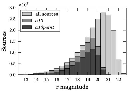
r-band magnitude distribution for all objects in the catalogue (light grey). Overlaid we also show the distribution for objects detected at S/N > 10 in all bands selected according to the quality criteria described in Table 6 (a10, grey), and for the set of unconfused 10σ point source detections described in Table 7 (a10point, dark grey). The distributions for i and Hα look identical, apart from being shifted by about 1 and 0.5 mag towards brighter magnitudes, respectively.
It is easy to see how the quality criteria may be adapted to be more tolerant. For example, by raising the allowed photometric uncertainties from 0.1 to 0.2 mag in Table 6, 42 million candidate sources would be added to the 109 million satisfying the tighter error bound. Our choice to adopt 0.1 mag as the cut-off uncertainty for the a10 category is a pragmatic trade-off which we found to suit many science applications, but users are encouraged to revise the quality criteria according to their needs.
6.3 Source reliability
Having obtained a set of quality criteria, we now assess how these improve the data quality. In this section, we start by discussing the reliability of the survey, which we define as the fraction of sources which are genuine astrophysical objects. To estimate the reliability, we cross-matched IPHAS against SDSS DR7,10 which is a catalogue of similar resolution and depth. By computing the fraction of IPHAS sources which were also independently detected by SDSS, we can obtain a good lower limit on the reliability.
The comparison was carried out across three cone-shaped regions, each covering 1 deg2, using a strict cross-matching distance of 0.5 arcsec. We considered four subsets of the IPHAS catalogue:
the entire (unfiltered) catalogue;
objects detected in all three bands;
a10 sources;
a10point sources.
The results for each of the regions and subsets are presented in Table 8. We find that our catalogue shows a good baseline reliability (90.8 per cent), which is improved markedly by the simple requirement that a source needs to be detected in all three bands (98.7 per cent). Reliabilities of 99.5 and 99.7 per cent are achieved using the a10 and a10point quality flags.
Fractions of sources in our catalogue which are also found in SDSS DR7 within a cross-matching radius of 0.5 arcsec. These percentages can be interpreted as lower limits for the reliability of our sources, i.e. the probability that an entry in our catalogue is a genuine astrophysical source rather than an instrumental artefact. The fractions were computed in three 1 deg2 regions where both surveys show contiguous overlap. The reliability is shown without quality criteria applied (‘all’), using only objects detected in all three bands (nBands = 3), using objects detected at 10σ in all three bands (a10), and finally using objects classified as reliable 10σ point sources (a10point).
| Region (ℓ, b) | all | nBands = 3 | a10 | a10point |
|---|---|---|---|---|
| (149.39, 4.06) | 93.0 per cent | 98.8 per cent | 99.7 per cent | 99.8 per cent |
| (186.59, −2.50) | 90.0 per cent | 98.8 per cent | 99.4 per cent | 99.6 per cent |
| (202.70, −1.75) | 89.4 per cent | 98.5 per cent | 99.4 per cent | 99.7 per cent |
| Mean | 90.8 per cent | 98.7 per cent | 99.5 per cent | 99.7 per cent |
To understand the nature of the small fraction of a10point-flagged sources which appear to be unreliable in this test, we investigated the data by eye. We found these ‘unreliable’ objects to be located in the vicinity of moderately bright stars (r ≲ 12), tracing out an area which is affected by saturation spikes or scattered light in the SDSS images. In all cases, we found these remaining objects to appear as genuine stars in both the IPHAS and SDSS images. It is hence likely that the reliability of the a10point class is close to 100 per cent.
6.4 Random and systematic uncertainties
Fig. 12 shows the mean photometric uncertainties (rErr, iErr, haErr) as a function of magnitude. We find the typical uncertainty to reach 0.1 mag near r = 20.5 and i, Hα = 19.5. We note that the fainter depth in r is compensated by the fact that most stars have brighter magnitudes in i and Hα; the average colours in the catalogue are |$\overline{(r-i)}=1.06\pm 0.12$| and |$\overline{(r-{H\alpha})}=0.44\pm 0.03$|. We warn that the statistics shown in Fig. 12 are the random errors based on the expected Poissonian photon noise. Systematics, such as calibration and deblending errors, are not included.
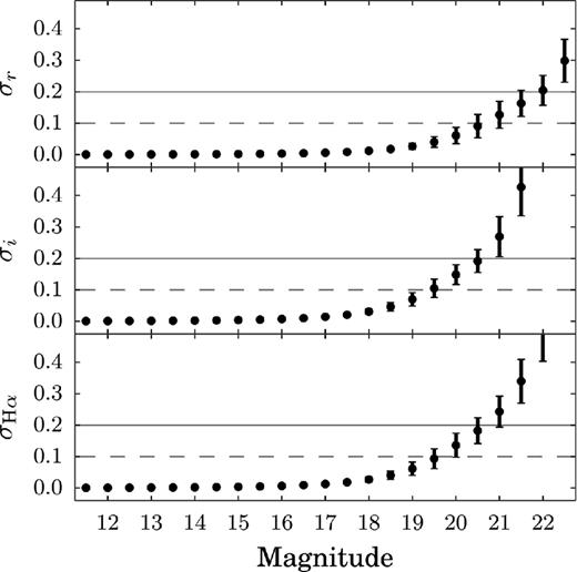
Mean photometric uncertainties for r (top), i (middle), and Hα (bottom). Data points shown are the average values of columns rErr, iErr, and haErr in the catalogue, and the error bars show the standard deviations. The dashed and solid lines indicate the 10σ and 5σ limits, respectively. These statistics show the average level of the Poissonian photon noise and do not include systematic uncertainties.
To appraise the level at which our photometry is affected by such systematics, we can exploit the secondary measurements which are present in the catalogue (i.e. r versus r2, i versus i2, ha versus ha2). In Fig. 13(a), we show the mean absolute residuals between these primary and secondary magnitudes as a function of magnitude (black dots). We also plot the Poissonian uncertainties for comparison (solid red line). We find the mean residual and standard deviation to be 0.03 ± 0.04 mag across the magnitude ranges 13–18 (r) and 12–17 (i, Hα), which is consistent with the accuracy of the calibration. Stars fainter than this range appear to be dominated by photon noise (red line), while stars at the bright end appear to suffer from large systematic errors due to saturation effects.
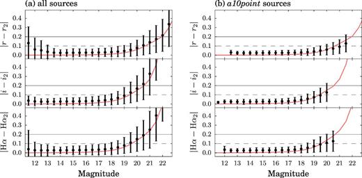
Photometric repeatability as a function of magnitude for all sources in the catalogue (panel a) and for the a10point sources alone (panel b). Black dots show the mean absolute residuals between the primary and the secondary detections. The error bars show the standard deviations. The red trend line shows the average Poissonian uncertainties we derived in Fig.. We find that the a10point quality criteria are successful at removing objects with large residuals.
In Fig. 13(b), we show a similar comparison between the primary and secondary detections, but this time we have only included sources which are flagged as a10point in the catalogue. We do not observe an improvement in the average residuals as a function of magnitude, but the number of outliers has decreased markedly (evidenced by the shorter error bars which denote the standard deviation of the absolute residuals). We conclude that the a10point quality criteria are effective at reducing the level of the systematic errors, while also removing the inaccurate data at the bright and faint end.
6.5 Source counts and blending
Fig. 14 shows the number of sources in the catalogue counted in 1°-wide strips as a function of Galactic longitude (thick blue line). Unsurprisingly, we find the number of sources to increase towards the Galactic Centre. For example, the average source density near ℓ ≃ 30° is roughly 300 000 objects per square degree, which is six times more than the density found near ℓ ≃ 180°. In addition to the global trend, variations are also apparent on smaller scales. For example, we find a significant drop near the constellations of Aquila (ℓ ≃ 40°) and Cygnus (ℓ ≃ 80° and ≃ 90°), which are regions known to be affected by high levels of foreground extinction (the extremities of ‘the Great Rift’; e.g. Bok & Bok 1941). However, we warn that the source counts shown have not been corrected for field pairs that have yet to be released or for variations in the depth across the included fields. For example, the dip near ℓ ≃ 140° is an artificial feature caused by gaps in the footprint coverage (seen in Fig. 2).
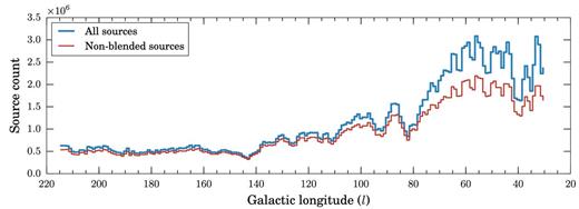
Number of entries in the IPHAS DR2 source catalogue as a function of Galactic longitude. The upper blue line shows the number of sources counted in 1°-wide longitude bins. The lower red line uses the same binning but includes only those sources for which the deblend flag is FALSE, i.e. unconfused sources for which the CASU pipeline did not have to apply a deblending procedure. In both cases, we counted only those sources in the latitude range −5° < b < +5° such that one may obtain a rough guide to source density by dividing the counts by 10 deg2. The global variations in the source counts traces the structure of the Galaxy and the distribution of foreground extinction, but is also affected by instrumental effects such as variations in the observed depth and completeness (see text).
In a forthcoming paper, properly calibrated detailed maps of stellar density of the northern Galactic plane will be presented (Farnhill et al., in preparation). This will incorporate completeness corrections based on the statistics of artificial source recovery. Such maps are of interest as tests of Galactic models.
Fig. 14 also shows the number counts for non-blended sources (thin red line). These are sources for which the deblend flag is FALSE, i.e. sources for which the CASU pipeline did not have to apply a deblending procedure to separate the flux originating from two or more overlapping objects. This provides some insight into how the fraction of blend-affected sources correlates with the local source density. In headline numbers, only 11 per cent of the sources are blended at ℓ > 90°, whereas 24 per cent are blended at ℓ < 90°.
Finally, we warn that blended objects are more likely than unblended objects to have fallen victim to source confusion during the band-merging procedure. It is important to bear this in mind when appraising stars of seemingly unusual colours (such as candidate emission-line stars) – if blending is flagged, the probability that the unusual colour is spurious is greatly increased.
7 DEMONSTRATION
We conclude this paper by demonstrating how the unique (r − Hα, r − i) colour-colour diagram offered by this catalogue can readily be used to (i) characterize the extinction regime along different sightlines, and (ii) identify Hα emission-line objects.
7.1 Colour-colour and colour-magnitude diagrams
The survey's unique (r − Hα) colour, when combined with (r − i), has been shown to provide simultaneous constraints on intrinsic stellar colour and interstellar extinction (Drew et al. 2008). Put differently, the main sequence in the (r − Hα, r − i) diagram runs in a direction that is at a large angle relative to the reddening vector, because the (r − Hα) colour tends to act as a coarse proxy for spectral type and is less sensitive to reddening than (r − i). As a result, the distribution of a stellar population in the IPHAS colour–colour diagram can offer a handle on the properties of the population and the extinction along a line of sight.
This is demonstrated in Figs 15, 16, and 17, where we present three sets of IPHAS colour/magnitude diagrams towards three distinct sightlines located at Galactic longitudes 180°, 45° and 30°, respectively, which were chosen because they show stellar populations with different characteristics. Each figure contains all the sources flagged as a10point within a region of 1 deg2 centred on the coordinates indicated in the diagram (i.e. within a radius of 0| $_{.}^{\circ}$|564 from the indicated sightline). For clarity, we have imposed the additional criterion that the photometric uncertainties must be smaller than 0.05 mag in each band, corresponding to a cut-off near 19th magnitude.
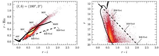
Colour–colour and colour–magnitude diagrams (left- and right-hand panel) showing sources flagged as a10point located in an area of 1 deg2 centred near the Galactic anticentre at (l, b) = (180°, +3°). The diagrams are plotted as 2D histograms which show the density of objects in bins of 0.01-by-0.01 mag; bins containing 1–10 objects are coloured red, while bins with more than 20 objects are yellow. The left-hand panel is annotated with the position of the main sequence (thin solid line), giant stars (thick solid line), and the reddening track for an A0V-type star (dashed line). The right-hand panel shows the unreddened 1 Gyr isochrone from the models by Bressan et al. (2012, solid line) along with the reddening vector for an A0V type (dashed line), both placed at an arbitrary distance of 2 kpc. This is one of the least reddened sightlines in the survey and hence the observed stellar population appears to be dominated by lowly reddened main-sequence stars (see text).
Same as above for (l, b) = (45°, +2°), which is one of the highest density sightlines in the survey, revealing two groups of stars in colour–magnitude space.
Same as above for (l, b) = (30°, 0°), showing one of the most reddened sightlines in the survey.
Each of the diagrams reveals a well-defined locus, which helps to further demonstrate the health of the catalogue and the global calibration for investigating stellar populations across wide areas. We have annotated the colour–colour diagrams by showing the position of the unreddened main sequence (thin solid line), the unreddened giant branch (thick solid line), and the reddening track for an A0V-type star (dashed line) – all three are based on the Pickles (1998) library of empirical spectra synthesized into the Vega-based IPHAS system by Drew et al. (2005). In the colour–magnitude diagrams, we only show the reddening vector together with the unreddened 1 Gyr isochrone due to Bressan et al. (2012), which is made available for the IPHAS system through the online tool hosted at the Observatory of Padova (http://stev.oapd.inaf.it/cmd). The isochrone and reddening vector have been placed at an arbitrary distance of 2 kpc.
Each of the sightlines reveals a stellar population with distinct characteristics. Towards the Galactic anticentre at ℓ = 180° (Fig. 15), we find a population dominated by lowly reddened main-sequence stars. This is consistent with the estimated total sightline extinction of E(B − V) = 0.49 given by Schlegel, Finkbeiner & Davis (1998), and applying the 14 per cent reduction recommended by Schlafly & Finkbeiner (2011). Looking in more detail, we can see that the stellar locus is narrower for M-type dwarfs than for earlier types: we do not observe M dwarfs experiencing the strongest reddening possible for this sightline. This implies that extinction is still increasing at distances of ∼1–2 kpc, where M dwarfs become too faint to be contained in the IPHAS catalogue. It is also clear that there are no unreddened stars earlier than ∼K0 visible; such stars would be saturated if within a few hundred parsecs. This therefore suggests that there is a measurable increase in extinction locally. We also note a relative absence of late-type giants which, due to the relative brevity of the corresponding phase of stellar evolution, would only account for a small proportion of this more nearly volume-limited sample seen in the anticentre direction.
In contrast, lines of sight passing into the first Galactic quadrant yield samples that are more commonly magnitude limited instead. For example, at ℓ = 45° (Fig. 16), there is a wealth of reddened objects and late-type giants. In the colour–magnitude diagram, it is clear that the stars are split into two distinct groups, with one significantly redder than the other. The bluer group is composed of main-sequence stars, with the slope of this group in the colour–magnitude diagram attributable to the significantly increasing extinction. Meanwhile, the redder group is principally composed of red giant stars (see Wright et al. 2008). As these stars are intrinsically brighter, they will be substantially further away than their main-sequence counterparts at the same apparent magnitude. Given that extinction continues to increase with distance, along this sightline, the red giants we observe will be subject to appreciably more reddening than the main-sequence stars, pushing them to (r − i) ∼ 1.5.
Finally, in one of our lowest longitude sightlines at ℓ = 30°, we find a very high number of extremely reddened giants in addition to an unreddened population of foreground dwarfs. In contrast to the sightline at ℓ = 45°, there is no clear group of giant stars visible in the colour–magnitude diagram of Fig. 17, although the red clump stars are manifested as a track of slight overdensity sitting roughly 0.4 mag redder than the A0V reddening track. At (l, b) = (45°, +2°), the giant stars observed exhibit a relatively narrow range of reddenings as they lie beyond most of the Galactic dust column. At (l, b) = (30°, 0°), this is not the case: even at the substantial distances at which we can observe reddened giant stars, extinction is continuing to rise within the Galactic mid-plane. It is also apparent that the (r − i) width of both the M dwarfs and early A dwarfs is greater than that in Fig. 16. This is indicative of a steeper rise in reddening, both within several hundred parsecs (M dwarfs) and within a few kpc (early A dwarfs).
These are just descriptive vignettes of the information obtainable from IPHAS colour–colour and colour–magnitude plots. A more rigorous quantitative analysis of the IPHAS catalogue can be undertaken to estimate both the stellar density distribution in the Milky Way (Sale et al. 2010) and to create detailed three-dimensional maps of the extinction across several kpc (Sale et al. 2009; Sale 2012). A 3D extinction map based on the DR2 catalogue is being released in a separate paper (Sale et al. 2014).
7.2 Identifying Hα emission-line objects
An aim of IPHAS is to enable the discovery of new fainter emission-line objects across the Galactic plane. The survey-wide identification and analysis of emission-line objects is beyond the scope of this work and will be the focus of a forthcoming paper (Barentsen et al., in preparation). In this section, we merely aim to demonstrate a use of the catalogue for this purpose.
An initial list of candidate Hα emitters based on the first IPHAS data release was previously presented by Witham et al. (2008). Because no global calibration was available at the time, Witham et al. employed a sigma-clipping technique to select objects with large, outlying (r − Hα) colours. In contrast, the new catalogue allows objects to be picked out from the (r − Hα, r − i) colour–colour diagram using model-based colour criteria rather than an adaptive statistical procedure. In what follows, we demonstrate this new capability by selecting candidate emission-line objects towards a small region in the sky.
The target of our demonstration is Sh 2-82: a 5-arcmin-wide |${\rm H\,\small {II}}$| region located near (l, b) = (53| $_{.}^{\circ}$|55, 0| $_{.}^{\circ}$|00) in the constellation of Sagitta. Nicknamed by amateur astronomers as the ‘Little Cocoon Nebula’, Sh 2-82 is ionized by the ∼10th magnitude star HD 231616 with spectral type B0V/III (Georgelin, Georgelin & Roux 1973; Mayer & Macák 1973; Hunter & Massey 1990). This ionizing star has been placed at a likely distance of 1.5–1.7 kpc based on its photometric parallax (Mayer & Macák 1973; Lahulla 1985; Hunter & Massey 1990).
Fig. 18 shows a 20-by-15 arcmin colour mosaic centred on Sh 2-82, composed of our Hα (red channel), r (green channel), and i (blue channel) images. The ionizing star can be seen as the bright object in the centre of the |${\rm H\,\small {II}}$| region, which is surrounded by a faint reflection nebula and several dark cloud filaments. For comparison, Fig. 19 shows a mosaic of the same region as seen in the mid-infrared by the Spitzer Space Telescope Galactic Legacy Infrared Mid-Plane Survey Extraordinaire (GLIMPSE; Benjamin et al. 2003; Churchwell et al. 2009). The infrared image reveals an enclosing fuzzy bubble (appearing green in Fig. 19) which is thought to originate from the mid-infrared emission of polycyclic aromatic hydrocarbons – i.e. warm dust – which is frequently observed at the interface between neutral regions of interstellar material and the ionizing radiation from early-type stars (Churchwell et al. 2006). Yu & Wang (2012) recently noted that the warm dust surrounding Sh 2-82 appears to contain infrared-bright YSOs. Many of these young objects appear as red- and pink-coloured stars in Fig. 19, located predominantly in the top-left part of the bubble.
IPHAS image mosaic of |${\rm H\,\small {II}}$| region Sh 2-82, composed of Hα (red channel), r (green channel), and i (blue channel). Yellow triangles show the position of candidate Hα emitters which have been selected from the colour–colour diagram in Fig. 20.

Star-forming region Sh 2-82 as seen in the mid-infrared by the Spitzer Space Telescope. The mosaic is composed of the 24 μm (red), 8.0 μm (green), and 4.5 μm (blue) bands. The image reveals a bubble-shaped structure which surrounds the Hii region that is seen in the IPHAS mosaic which spans the same region (Fig. 18). This structure has previously been labelled as N115 in the catalogue of Churchwell et al. (2006), and could be a possible site of triggered star formation (Kendrew et al. 2012; Thompson et al. 2012).
Fig. 20 presents the IPHAS colour–colour diagram for the 20-by-15 arcmin region shown in the mosaics. Grey circles show all objects which are brighter than r < 20 and have been flagged as a10 in IPHAS DR2. The diagram also shows the unreddened main sequence (solid line) and the expected position of unreddened main-sequence stars with Hα in emission at a strength of EW =−10 Å (dashed line). Six stars are found to lie above the dashed line at the level of 3σ, i.e. the distance between the objects and the dashed line is larger than three times the uncertainty in their (r − Hα) colour. These candidate Hα emitters are marked by red triangles in the colour–colour diagram, and by yellow triangles in the image mosaic (Fig. 18). Their details are listed in Table 9.
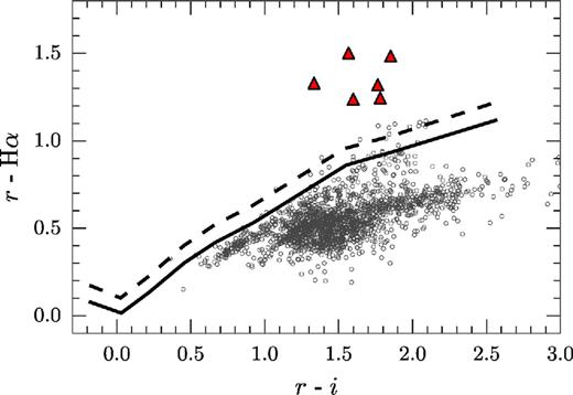
(r − Hα, r − i) diagram for the rectangular region of 20-by-15 arcmin centred on the H ii region Sh 2-82, which is the area shown in Fig. 18. The diagram shows all objects in the catalogue which have been flagged as a10 and are brighter than r < 20 (grey circles). The unreddened main sequence is indicated by a solid line, while the main sequence for stars with an Hα emission-line strength of − 10 Å EW is indicated by a dashed line (both based on the colour simulations by Barentsen et al. 2011). Red triangles indicate objects which have been identified as likely Hα emitters.
Candidate Hα emitters towards Sh 2-82.
| # | Name (IPHAS2...) | r | i | Hα |
|---|---|---|---|---|
| 1 | J192954.40+181026.1 | 17.69 ± 0.01 | 16.12 ± 0.01 | 16.19 ± 0.01 |
| 2 | J193011.01+182051.2 | 18.55 ± 0.02 | 16.95 ± 0.02 | 17.31 ± 0.02 |
| 3 | J193021.52+181954.5 | 19.72 ± 0.05 | 17.94 ± 0.03 | 18.47 ± 0.04 |
| 4 | J193024.45+181938.3 | 19.31 ± 0.04 | 17.55 ± 0.02 | 17.99 ± 0.03 |
| 5 | J193033.00+181609.3 | 18.25 ± 0.01 | 16.91 ± 0.01 | 16.92 ± 0.01 |
| 6 | J193042.48+182317.4 | 19.96 ± 0.03 | 18.11 ± 0.03 | 18.48 ± 0.03 |
In previous work, we have shown that the majority of Hα emitters seen by IPHAS towards an |${\rm H\,\small {II}}$| region are likely to be Classical T Tauri Stars (Barentsen et al. 2011). These are young objects which are thought to show Hα in emission due to the presence of hot, infalling gas which is accreting on to the star from a circumstellar disc. This is likely to be the case for the candidate Hα emitters we discovered towards Sh 2-82 as well. Two of our candidates, #1 and #4 in Table 9, have previously been identified as candidate YSOs by Robitaille et al. (2008) and Yu & Wang (2012), respectively. In these studies, the authors used Spitzer data to find intrinsically red objects, with SEDs consistent with the presence of a circumstellar disc. Although the other four candidate emitters in our sample have not previously appeared in the literature, we note that all four are detected in the Spitzer 8.0-μm image at S/N > 5. They are likely to be YSOs exhibiting a mild infrared excess. The recovery of Hα emitters in Spitzer data illustrates how IPHAS can complement infrared surveys.
7.3 IPHAS as a complement to infrared data
Towards Sh2-82, the IPHAS and Spitzer/GLIMPSE catalogues have 4798 entries in common, out of 10 739 and 11 321 entries in total, respectively. Fig. 21 presents the Spitzer colour–colour diagram of the region, showing the 1356 objects that were detected in all four GLIMPSE bands. We have indicated the 845 objects (62 per cent) that have a counterpart in IPHAS (grey circles) and the 511 objects that do not (red crosses).
Spitzer/GLIMPSE colour–colour diagram towards Sh 2-82, showing the objects for which a counterpart exists in IPHAS (845 objects, grey circles) and those for which no counterpart was identified (511 objects, red crosses). A cross-matching radius of 1 arcsec was used to identify counterparts. The arrow illustrates the reddening vector corresponding to AKs = 3 following the reddening law due to Flaherty et al. (2007). It is apparent that objects near the top of the diagram, where heavily reddened objects are expected to sit, tend to have no counterpart. In contrast, many of the objects on the right-hand side of the diagram, where YSOs are expected to sit, do have counterparts.
We find that objects located in the upper half of the Spitzer diagram are less likely to have an IPHAS counterpart, which is where highly reddened objects are expected to sit. Moreover, amongst the objects with a counterpart, we note that more have been detected in i (843 objects) than in r (634) or Hα (600). This is not surprising, because Sh2-82 is located towards a high-extinction sightline near the inner plane, where an optical survey will naturally be extinction limited. Nevertheless, the extinction map due to Sale et al. (2014) has demonstrated that IPHAS can probe stars as far away as 4–5 kpc towards this region. The situation will be even more favourable in the outer plane, where dust optical depths are low.
We note that Sh 2-82 is one of a large population of poorly studied star-forming regions located at low Galactic latitudes, which have only recently started to become revealed by efforts to catalogue the wealth of ‘bubbles’ detected at mid-infrared wavelengths (Churchwell et al. 2006; Simpson et al. 2012), and by efforts to catalogue previously unknown clusters seen in the near-infrared (e.g. Bica et al. 2003). IPHAS data can offer a handle on the extinction, distance, and stellar contents of many of such unexplored regions.
7.4 r − Hα excess as a quantitative measure of Hα emission
As well as discovering emission-line stars, IPHAS data can provide a first estimate of the equivalent width (EW) of line emission. How this is done has been discussed in previous works – most notably by Drew et al. (2005) and more recently by Barentsen et al. (2011). Given that the narrow-band filter used has an FWHM of 95 Å, it is to be expected that the appearance in a spectrum of line emission corresponding to an EW of 95 Å would increase r − Hα by 0.75 mag (i.e. the flux captured within the narrow-band doubles). Similarly, 10 Å of line emission should increase r − Hα by 0.11 mag.
This simple reasoning breaks down when the Hα emission becomes so bright that it also dominates the flux captured across the entire r broad-band. It was noted by Drew et al. (2005) that the very bright line limiting value of r − Hα is ∼3.1 in the Vega system. This fact, on its own, implies that any apparent detection of an Hα emission-line star without a corresponding r detection is only real if the Hα magnitude is not brighter by more than 3.1 mag relative to the r detection limit (i.e. typically, credible Hα-only sources must be fainter than ∼18th mag).
In order to infer the emission EW from the r − Hα colour, it is necessary to know the value this colour would have in case of no excess line emission. In the general case, this is not possible without some prior knowledge of the star's reddening and spectral type (i.e. the inferences drawn for an unreddened M dwarf or a reddened F star would not be the same – the absolute value of the EW in the latter case would be greater because the reddened F star without emission would lie at lower r − Hα). This is the situation faced in the study of IC 1396 by Barentsen et al. (2011) in which Hα EWs were inferred relative to a reddened sequence of K–M stars appropriate to this star-forming region. A different choice of reddening would have resulted in different EW estimates.
However, it was found by Drew et al. (2005) that for earlier type stars in which the spectrum is not heavily modulated by line features or molecular bands the estimation of net emission EW is more straightforward and unambiguous. It was demonstrated, for spectral slopes ranging from the Rayleigh–Jeans limit to that appropriate to an early G star and for a range of reddenings, that it is possible to draw a unique set of constant EW lines in the (r − Hα, r − i) diagram that can be compared directly with the positions of candidate emission-line stars, thereby predicting emission EW (see Fig. 6; Drew et al. 2005). The EW in this case should be understood to be the measure of the emission observed above the interpolated continuum (i.e. no correction is present for any assumed infilled photospheric line absorption).
In Fig. 22, we show how well this works in reality: the predicted lines of constant emission EW in the (r − Hα, r − i) plane are compared with the positions of a sample of over 200 classical Be stars in Perseus (from Raddi et al. 2014). Stars of this type come with the advantage that secular variation, whilst it certainly occurs, is not as common as in T Tau stars. The objects plotted are a bright selection (r ≲ 16.5) for which there are spectroscopic determinations of Hα emission EW. A colour scale has been applied to the data points that darkens as EW increases. The gradation apparent in the shading of the data points follows the trend set by the constant EW lines quite well. The experience has been that the EW deduced from IPHAS photometry for individual objects is commonly within 10 Å of subsequent spectroscopic measurement (see also fig. 5 of Barentsen et al. 2011). Evidently, the photometry is well suited to statistical measurement across large samples, while for individual objects a useful approximation is delivered.
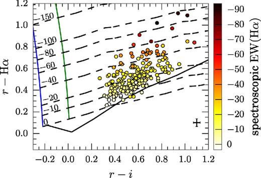
Photometric predictions of Hα EW compared with spectroscopic measurements of a sample of classical Be stars (from Raddi et al. 2014). The broken lines are predicted lines of constant net emission EW, while the analogous spectroscopic EW is represented by the colouring of the data points. The unreddened main sequence, which normally serves as the upper bound to the main stellar locus, is drawn as a solid black line. Strongly reddened stars with not-so-strong line emission will fall below it and be hard to pick out without additional information. The two vertical lines drawn are ‘curves of growth’ showing how r − Hα increases – and r − i drops a little – as more and more line emission is added, raising the flux in Hα narrow-band and to a lesser proportion the flux in the r band. The blue line represents the trend for an unreddened Rayleigh–Jeans continuum (with superposed Hα emission), while the green line is the trend for the case of an unreddened A0 continuum.
8 CATALOGUE AND IMAGE ACCESS
The catalogue will be made available through the Vizier service (http://cdsweb.u-strasbg.fr/cgi-bin/qcat?II/321), where it can be queried using a web interface and using Virtual Observatory protocols. In addition, the catalogue can be downloaded in its entirety from our website as a collection of binary FITS tables, each covering a 5° × 5° tile of the footprint and comprising 50 GB in total (see www.iphas.org/dr2).
To estimate absolute narrow-band Hα fluxes from the image data, we note that the integrated in-band energy flux for Vega in the IPHAS Hα filter is 1.52 × 10⁻⁷ erg cm−2 s−1 at the top of the Earth's atmosphere, which is the flux obtained by folding the CALSPEC SED with the filter transmission curve only (the correction for atmosphere and detector quantum efficiency, otherwise scales down the narrow-band flux by 0.707). This implies that the in-band flux corresponding to zero magnitude is 1.56 × 10⁻⁷ erg cm−2 s−1, when the Hα magnitude for Vega is set by convention to 0.03 (Fukugita et al. 1996). These flux estimates are consistent with the most recent version of Vega's SED presented by Bohlin (2014).
We warn that the image repository on our website includes data that did not pass quality control and has not been globally re-calibrated. Such data are flagged in the online meta data table, which is available from our website, and must be used with great caution.
In the spirit of reproducibility, the source code that was used to generate the catalogue is made available at https://github.com/barentsen/iphas-dr2
9 CONCLUDING REMARKS AND FUTURE WORK
A new catalogue has been derived from IPHAS. It is the first to offer comprehensive CCD photometry of point sources across the northern Galactic plane at visible wavelengths, taking in the Galactic latitude range |b| < 5° at longitudes ℓ = 30°–215°. The new 99-column catalogue provides single-epoch photometry across 92 per cent of the survey area, and is the first quality-controlled and globally calibrated catalogue to have been constructed from the imaging data. This now means that there is Hα coverage, accessible online, of the entire Galactic plane – given that the southern plane is already available thanks to the UK Schmidt Hα Survey (SHS; Parker et al. 2005), the last of the photographic surveys carried out by that telescope.
The observations included in this release achieve a median seeing of 1.1 arcsec and 5σ depths of r = 21.2 ± 0.5, i = 20.0 ± 0.3, and Hα = 20.3 ± 0.3. The global calibration and photometric repeatability are found to be accurate at the level of 0.03 mag (rms), providing a significant improvement over the previous data release. The source catalogue specifies the best-available single-epoch astrometry and photometry for 219 million unique sources. To support its exploitation, we provide a list of recommended quality criteria that will permit the selection of objects with accurate colours from the catalogue. The closing demonstrations highlight the use of the survey's unique (r − Hα, r − i) diagram for characterizing stellar populations and selecting emission-line objects. More comprehensive applications of IPHAS can be found in the works of Sale et al. (2014), which applies DR2 to the problem of 3D extinction mapping, and of Sabin et al. (2014), where the results of a search of the image data base for new planetary nebulae are presented.
The current plan is to work towards one further major IPHAS source catalogue, in which the remaining gaps in sky coverage will have been eliminated – observations aimed at replacing data not meeting the quality requirements are continuing. We will also examine options to further improve the global calibration, perhaps tightening the accuracy to better than 2 per cent. For example, we have in mind investigating the use of the PanSTARRS photometric ladder (Magnier et al. 2013) as a reference set, when it becomes available for the Galactic plane, and we will explore improving source recovery in the most dense fields via the implementation of PSF fitting in place of aperture photometry. Finally, the next catalogue will detail all the secondary detections to aid time-domain studies.
The data-taking strategy developed for IPHAS has since been reapplied to carry out a companion INT/WFC Galactic Plane survey called UVEX in U, g, r, He i (Groot et al. 2009), a survey of the Kepler field in U, g, r, i, Hα (Greiss et al. 2012), and a survey of the southern Galactic plane and bulge in u, g, r, i, Hα called VPHAS+ (Drew et al. 2014). The last of these incorporates the digital update of the SHS, offering all the advantages of calibrated photometry across a little over half the SHS footprint. The work presented here stands as a potential template for the catalogues that remain to be generated from these sibling surveys. In prospect from them, whether they are mined separately or together, are the means to ask seamless questions on the contents and structure of the most highly populated components of the Milky Way.
ACKNOWLEDGEMENTS
The INT is operated on the island of La Palma by the ING in the Spanish Observatorio del Roque de los Muchachos of the Instituto de Astrofísica de Canarias. We are deeply indebted to Ovidiu Vaduvescu, Javier Méndez, and the rest of the ING staff and students for their ongoing support of the telescope. All data were processed by the CASU at the Institute of Astronomy in Cambridge. The catalogue presented in this work was assembled at the Centre for Astrophysics Research, University of Hertfordshire, supported by a grant from the Science and Technology Facilities Council of the UK (STFC, ref ST/J001335/1).
Preparation of the catalogue was eased greatly by a number of software packages, including the postgresql data base software, the topcat and stilts packages (Taylor 2005, 2006), and the python modules astropy (Astropy Collaboration et al. 2013), numpy and scipy (Oliphant 2007), matplotlib (Hunter 2007), ipython (Pérez & Granger 2007), and aplpy. We also made use of the montage software maintained by NASA/IPAC, and the SIMBAD, VIZIER, and aladin services operated at CDS, Strasbourg, France (Bonnarel et al. 2000).
Our work made extensive use of several complementary photometric surveys. Our global calibration was aided by the APASS, funded by the Robert Martin Ayers Sciences Fund. The calibration was tested against the SDSS, funded by the Alfred P. Sloan Foundation, the Participating Institutions, the National Science Foundation, the US Department of Energy, the National Aeronautics and Space Administration, the Japanese Monbukagakusho, the Max Planck Society, and the Higher Education Funding Council for England. The astrometric pipeline reduction made significant use of the 2MASS, which is a joint project of the University of Massachusetts and the Infrared Processing and Analysis Center/California Institute of Technology, funded by NASA and the NSF. This work includes observations made with the Spitzer Space Telescope, which is operated by the Jet Propulsion Laboratory, California Institute of Technology under a contract with NASA.
GB, JED, SES, and BTG acknowledge support from the Science and Technology Facilities Council of the United Kingdom (grants: GB and JED – ST/J001333/1, SES – ST/K00106X/1, BTG – ST/I001719/1). HJF and MM-S both acknowledge STFC postgraduate studentships. JED would also like to convey her thanks to the Physics Department of Imperial College London that hosted this project from its inception to 2007 and supported her via a sabbatical year in 2003–04. JF is supported by the Spanish Plan Nacional de I+D+i and FEDER under contract AYA2010-18352. BTG acknowledges funding from the European Research Council under the European Union's Seventh Framework Programme (FP/2007-2013)/ERC Grant agreement no. 320964 (WDTracer). PRG is supported by a Ramón y Cajal fellowship (RYC-2010-05762), and acknowledges support provided by the Spanish MINECO AYA2012–38700 grant. NJW is in receipt of a Fellowship funded by the Royal Astronomical Society of the United Kingdom.
We are grateful to the anonymous referee for the insightful feedback, which has helped us to improve the presentation of the data products.
The r-band exposure time was 10 s instead of 30 s in the first months of data taking. Since 2010 October, the i-band exposure time has been increased from 10 to 20 s to by-pass a sporadic exposure timing bug that affects the WFC.
We defined the 5σ limiting magnitude as the magnitude which a point source would have if its flux equalled five times the level of the noise in the sky background. The sky noise was estimated using a robust MAD estimator for noise scaled to equivalent Gaussian standard deviation, i.e. = MAD × 1.48, after removing large-scale sky background variations. (MAD = Median of the Absolute Deviations about the median.)
http://catserver.ing.iac.es/filter/list.php?instrument=WFC where the filters are named WFCH6568, WFCSloanR, and WFCSloanI.
‘ubercalibration’ refers to the name of the code used to re-calibrate SDSS photometry. It is an anglicized version of the German word ‘überkalibration’, which was reportedly chosen because the initial authors, Schlegel and Finkbeiner, both have German-sounding names (Finkbeiner 2010).
We used the CasJobs facility located at http://skyserver.sdss3.org/CasJobs to obtain photometry from the SDSS PHOTOPRIMARY table with criteria TYPE = STAR, CLEAN = 1 and SCORE > 0.7.
For consistency with the terminology that is used in the CASU pipeline and the WSA/VSA archives, extended objects are classified as ‘galaxies’. This class will flag any type of resolved object, however.
SDSS DR7 was chosen due to an apparent change in the catalogue preparation for DR8 and DR9, which resulted in fewer genuine stars being detected near bright (r < 12) sources, which in turn gave an unduly pessimistic view on our reliability.
REFERENCES
APPENDIX A: CATALOGUE FORMAT
Definition of columns in the IPHAS DR2 source catalogue.
| # | Column | Type | Unit | Description |
|---|---|---|---|---|
| 1 | name | String | Position-based source name in the sexagesimal form: ‘JHHMMSS.ss+DDMMSS.s’. You need to add the prefix ‘IPHAS2’ followed by a whitespace to obtain the official name ‘IPHAS2 JHHMMSS.ss+DDMMSS.s’ (where ‘J’ indicates that the position is J2000 equatorial and ‘IPHAS2’ indicates DR2). | |
| 2 | ra | Double | deg | J2000 right ascension with respect to the 2MASS PSC reference frame, which is consistent with ICRS to within 0.1 arcsec. The coordinate given is obtained from the astrometric measurement in the r-band exposure. If the source is undetected in r, then the i- or Hα-band coordinate is given. |
| 3 | dec | Double | deg | J2000 declination. See comments above. |
| 4 | sourceID | String | Unique identification number of the detection. Identical to rDetectionID if the source was detected in the r band. Identical to iDetectionID or haDetectionID otherwise. | |
| 5 | posErr | Float | arcsec | Astrometric rms residual measured against 2MASS across the CCD in which the source is detected. Be aware that the astrometric error for a source near the corner of a CCD may be significantly larger than the rms statistic. |
| 6 | l | Double | deg | Galactic longitude ℓ converted from RA/Dec. (IAU 1958 system). |
| 7 | b | Double | deg | Galactic latitude b converted from RA/Dec. (IAU 1958 system). |
| 8 | mergedClass | Short | Image classification flag based on all bands: 1=galaxy, 0=noise, −1=star, −2=probableStar, −3=probableGalaxy, −9=saturated. Computed using the UKIDSS scheme. | |
| 9 | mergedClassStat | Float | Merged N(0,1) stellarness-of-profile statistic. Computed using the UKIDSS scheme. | |
| 10 | pStar | Float | Probability that the source is a point source (value between 0 and 1). | |
| 11 | pGalaxy | Float | Probability that the source is an extended object, such as a galaxy, or a close blend of two point sources (value between 0 and 1). | |
| 12 | pNoise | Float | Probability that the source is noise, e.g. a cosmic ray (value between 0 and 1). | |
| 13 | rmi | Float | mag | (r − i) colour, formed by subtracting columns r and i. To obtain the uncertainty, take the root of the sum of the squares of columns rErr and iErr. |
| 14 | rmha | Float | mag | (r − Hα) colour, formed by subtracting columns r and ha. See comments above. |
| 15 | r | Float | mag | Default r-band magnitude using the 2.3-arcsec-diameter aperture. Calibrated in the Vega system. |
| 16 | rErr | Float | mag | Uncertainty for r. Does not include systematic errors. |
| 17 | rPeakMag | Float | mag | Alternative r-band magnitude derived from the peak pixel height (i.e. a 0.3 × 0.3 arcsec2 aperture). Calibrated in the Vega system. |
| 18 | rPeakMagErr | Float | mag | Uncertainty in rPeakMag. Does not include systematics. |
| 19 | rAperMag1 | Float | mag | Alternative r-band magnitude using the 1.2-arcsec-diameter aperture. Calibrated in the Vega system. |
| 20 | rAperMag1err | Float | mag | Uncertainty in rAperMag1. Does not include systematics. |
| 21 | rAperMag3 | Float | mag | Alternative r-band magnitude using the 3.3-arcsec-diameter aperture. Calibrated in the Vega system. |
| 22 | rAperMag3err | Float | mag | Uncertainty in rAperMag3. Does not include systematics. |
| 23 | rGauSig | Float | pixels | rms of axes of ellipse fit in r. |
| 24 | rEll | Float | Ellipticity in the r band. | |
| 25 | rPA | Float | deg | Position angle in the r band. |
| 26 | rClass | Short | Discrete image classification flag: 1=galaxy, 0=noise, −1=star, −2=probableStar, −3=probableGalaxy, −9=saturated. | |
| 27 | rClassStat | Float | N(0,1) stellarness-of-profile statistic. | |
| 28 | rDeblend | Boolean | True if the source is blended with a nearby neighbour in the r band. Although a deblending procedure is applied when measuring the photometry, the result may be unreliable (colours should not be trusted in particular). | |
| 29 | rSaturated | Boolean | True if the source is too bright to make an accurate measurement in the r band (e.g. peak pixel > 55 000 counts). The photometry is likely affected by systematic errors. | |
| 30 | rMJD | Double | d | Modified Julian Date at the start of the r-band exposure. |
| 31 | rSeeing | Float | arcsec | Average FWHM of stars in the same CCD frame. |
| 32 | rDetectionID | String | Unique identifier of the r-band detection in the format ‘|$\#$|run-|$\#$|ccd-|$\#$|number’, i.e. composed of the INT telescope run number, the CCD number, and a sequential source detection number. | |
| 33 | rX | Float | pixels | Pixel coordinate of the source in the r-band exposure, in the coordinate system of the CCD. |
| 34 | rY | Float | pixels | Pixel coordinate of the source in the r-band exposure, in the coordinate system of the CCD. |
| 35 | i | Float | mag | Default i-band magnitude using the 2.3-arcsec-diameter aperture. Calibrated in the Vega system. |
| 36 | iErr | Float | mag | Uncertainty for i. Does not include systematic errors. |
| 37 | iPeakMag | Float | mag | Alternative i-band magnitude derived from the peak pixel height (i.e. a 0.3 × 0.3 arcsec2 aperture). Calibrated in the Vega system. |
| 38 | iPeakMagErr | Float | mag | Uncertainty in iPeakMag. Does not include systematics. |
| 39 | iAperMag1 | Float | mag | Alternative i-band magnitude using the 1.2-arcsec-diameter aperture. Calibrated in the Vega system. |
| 40 | iAperMag1err | Float | mag | Uncertainty in iAperMag1. Does not include systematics. |
| 41 | iAperMag3 | Float | mag | Alternative i-band magnitude using the 3.3-arcsec-diameter aperture. Calibrated in the Vega system. |
| 42 | iAperMag3err | Float | mag | Uncertainty in iAperMag3. Does not include systematics. |
| 43 | iGauSig | Float | pixels | rms of axes of ellipse fit. |
| 44 | iEll | Float | Ellipticity. | |
| 45 | iPA | Float | deg | Position angle. |
| 46 | iClass | Short | Discrete image classification flag: 1=galaxy, 0=noise, −1=star, −2=probableStar, −3=probableGalaxy, −9=saturated. | |
| 47 | iClassStat | Float | N(0,1) stellarness-of-profile statistic. | |
| 48 | iDeblend | Boolean | True if the source is blended with a nearby neighbour in the i band. See comments for rDeblend above. | |
| 49 | iSaturated | Boolean | True if the source is too bright to make an accurate measurement in the i band. See comments for rSaturated above. | |
| 50 | iMJD | Double | d | Modified Julian Date at the start of the single-band exposure. |
| 51 | iSeeing | Float | arcsec | Average FWHM of stars in the same CCD frame. |
| 52 | iDetectionID | String | Unique identifier of the i-band detection in the format ‘|$\#$|run-|$\#$|ccd-|$\#$|number’, i.e. composed of the INT telescope run number, the CCD number, and a sequential source detection number. | |
| 53 | iX | Float | pixels | Pixel coordinate of the source, in the coordinate system of the CCD. |
| 54 | iY | Float | pixels | Pixel coordinate of the source, in the coordinate system of the CCD. |
| 55 | iXi | Float | arcsec | Position offset of the i-band detection relative to the ra column. The original i-band coordinates can be obtained by computing (ra+iXi/3600, dec+iEta/3600). |
| 56 | iEta | Float | arcsec | Position offset of the i-band detection relative to the dec column. See comments above. |
| 57 | ha | Float | mag | Default Hα magnitude using the 2.3-arcsec-aperture. Calibrated in the Vega system. |
| 58 | haErr | Float | mag | Uncertainty for ha. Does not include systematic errors. |
| 59 | haPeakMag | Float | mag | Alternative Hα magnitude derived from the peak pixel height (i.e. a 0.3 × 0.3 arcsec2 aperture). Calibrated in the Vega system. |
| 60 | haPeakMagErr | Float | mag | Uncertainty in haPeakMag. Does not include systematics. |
| 61 | haAperMag1 | Float | mag | Alternative Hα magnitude using the 1.2-arcsec-diameter aperture. Calibrated in the Vega system. |
| 62 | haAperMag1err | Float | mag | Uncertainty in haAperMag1. Does not include systematics. |
| 63 | haAperMag3 | Float | mag | Alternative Hα magnitude using the 3.3-arcsec-diameter aperture. Calibrated in the Vega system. |
| 64 | haAperMag3err | Float | mag | Uncertainty in haAperMag3. Does not include systematics. |
| 65 | haGauSig | Float | pixels | rms of axes of ellipse fit. |
| 66 | haEll | Float | Ellipticity. | |
| 67 | haPA | Float | deg | Position angle. |
| 68 | haClass | Short | Discrete image classification flag: 1=galaxy, 0=noise, −1=star, −2=probableStar, −3=probableGalaxy, −9=saturated. | |
| 69 | haClassStat | Float | N(0,1) stellarness-of-profile statistic. | |
| 70 | haDeblend | Boolean | True if the source is blended with a nearby neighbour in Hα. See comments for rDeblend above. | |
| 71 | haSaturated | Boolean | True if the source is too bright to make an accurate measurement in Hα. See comments for rSaturated above. | |
| 72 | haMJD | Double | d | Modified Julian Date at the start of the single-band exposure. |
| 73 | haSeeing | Float | arcsec | Average FWHM of stars in the same CCD frame. |
| 74 | haDetectionID | String | Unique identifier of the Hα detection in the format ‘|$\#$|run-|$\#$|ccd-|$\#$|number’, i.e. composed of the INT telescope run number, the CCD number, and a sequential source detection number. | |
| 75 | haX | Float | pixels | Pixel coordinate of the source, in the coordinate system of the CCD. |
| 76 | haY | Float | pixels | Pixel coordinate of the source, in the coordinate system of the CCD. |
| 77 | haXi | Float | arcsec | Position offset of the Hα detection relative to the ra column. The original Hα-band coordinates can be obtained by computing (ra+haXi/3600, dec+haEta/3600). |
| 78 | haEta | Float | arcsec | Position offset of the Hα relative to the ra column. See comments above. |
| 79 | brightNeighb | Boolean | True if a very bright star is nearby (defined as brighter than V<4 within 10 arcmin, or brighter than V<7 within 5 arcmin). Such very bright stars cause scattered light and diffraction spikes, which may add systematic errors to the photometry or even trigger spurious detections. | |
| 80 | deblend | Boolean | True if the source is blended with a nearby neighbour in one or more bands. Although a deblending procedure is applied when measuring the photometry, the result may be inaccurate and the colours should not be trusted. | |
| 81 | saturated | Boolean | True if the source is saturated in one or more bands. The photometry of saturated stars is affected by systematic errors. | |
| 82 | nBands | Short | Number of bands in which the source is detected (equals 1, 2, or 3). | |
| 83 | a10 | Boolean | True if the source is detected at S/N > 10 in all bands without being saturated, and if the photometric measurements are consistent across different aperture diameters. Algebraic condition: (rErr < 0.1 & iErr < 0.1 & haErr < 0.1 & NOT saturated & (abs(r −rAperMag1) < 3*hypot(rErr,rAperMag1Err)+0.03) & (abs(i −iAperMag1) < 3*hypot(iErr,iAperMag1Err)+0.03) & (abs(ha−haAperMag1) < 3*hypot(haErr,haAperMag1Err)+0.03). | |
| 84 | a10point | Boolean | True if both the a10 quality criteria above are satisfied, and if the object looks like a single, unconfused point source. Algebraic condition: a10 & pStar > 0.9 & NOT deblend & NOT brightNeighb. | |
| 85 | fieldID | String | Survey field identifier (e.g. 0001_aug2003). | |
| 86 | fieldGrade | String | Internal quality control score of the field. One of A, B, C, or D. | |
| 87 | night | Integer | Night of the observation (YYYYMMDD). Refers to the ut date at the start of the night. | |
| 88 | seeing | Float | arcsec | Maximum value of rSeeing, iSeeing, or haSeeing. |
| 89 | ccd | Short | CCD-chip number on the Wide Field Camera (WFC) of the INT. 1, 2, 3, or 4. | |
| 90 | nObs | Short | Number of repeat observations of this source in the survey. A value larger than 1 indicates that the source is unlikely to be spurious. | |
| 91 | sourceID2 | String | SourceID of the alternative detection of the object in the partner exposure. | |
| 92 | fieldID2 | String | FieldID of the partner detection (e.g. 0001o_aug2003). | |
| 93 | r2 | Float | mag | r-band magnitude in the dithered partner field, i.e. the dithered repeat measurement obtained within 10 min (if available). |
| 94 | rErr2 | Float | mag | Uncertainty for r2. |
| 95 | i2 | Float | mag | i-band magnitude in the dithered partner field, i.e. the dithered repeat measurement obtained within 10 min (if available). |
| 96 | iErr2 | Float | mag | Uncertainty for i2. |
| 97 | ha2 | Float | mag | Hα magnitude in the dithered partner field, i.e. the dithered repeat measurement obtained within 10 min (if available). |
| 98 | haErr2 | Float | mag | Uncertainty for ha2. |
| 99 | errBits2 | Integer | Error bit mask for the partner detection. Used to flag a bright neighbour (1), source blending (2), saturation (8), vignetting (64), truncation (128), and bad pixels (32 768). Be careful if errBits2 > 0. |
