


Abstract
We report results of a spectropolarimetric and photometric monitoring of the weak-line T Tauri star LkCa 4 within the Magnetic Topologies of Young Stars and the Survival of close-in giant Exoplanets (MaTYSSE) programme, involving ESPaDOnS at the Canada–France–Hawaii Telescope. Despite an age of only 2 Myr and a similarity with prototypical classical T Tauri stars, LkCa 4 shows no evidence for accretion and probes an interesting transition stage for star and planet formation. Large profile distortions and Zeeman signatures are detected in the unpolarized and circularly polarized lines of LkCa 4 using Least-Squares Deconvolution (LSD), indicating the presence of brightness inhomogeneities and magnetic fields at the surface of LkCa 4. Using tomographic imaging, we reconstruct brightness and magnetic maps of LkCa 4 from sets of unpolarized and circularly polarized LSD profiles. The large-scale field is strong and mainly axisymmetric, featuring a ≃2 kG poloidal component and a ≃1 kG toroidal component encircling the star at equatorial latitudes – the latter making LkCa 4 markedly different from classical T Tauri stars of similar mass and age. The brightness map includes a dark spot overlapping the magnetic pole and a bright region at mid-latitudes – providing a good match to the contemporaneous photometry. We also find that differential rotation at the surface of LkCa 4 is small, typically ≃5.5 times weaker than that of the Sun, and compatible with solid-body rotation. Using our tomographic modelling, we are able to filter out the activity jitter in the radial velocity curve of LkCa 4 (of full amplitude 4.3 km s−1) down to an rms precision of 0.055 km s−1. Looking for hot Jupiters around young Sun-like stars thus appears feasible, even though we find no evidence for such planets around LkCa 4.
1 INTRODUCTION
Magnetic fields are known to have a significant impact at early stages of evolution, when stars and their planets form from collapsing dense pre-stellar cores, progressively flattening into large-scale magnetized accretion discs and finally settling as pre-main-sequence (PMS) stars surrounded by protoplanetary discs (e.g. André, Basu & Inutsuka 2009; Donati & Landstreet 2009). At an age of 1–10 Myr, low-mass PMS stars have emerged from their dust cocoons and are still in a phase of gravitational contraction towards the main sequence (MS). They are either classical T-Tauri stars (cTTSs) when still surrounded by a massive (presumably planet-forming) accretion disc or weak-line T-Tauri stars (wTTSs) when their discs have mostly dissipated. Both cTTSs and wTTSs have been the subject of intense scrutiny at all wavelengths in recent decades given their interest for benchmarking the scenarios currently invoked to explain low-mass star and planet formation.
Magnetic fields of cTTSs play a key role in controlling accretion processes and in triggering outflows, and thus largely dictate the angular momentum evolution of low-mass PMS stars (e.g. Bouvier et al. 2007; Frank et al. 2014). More specifically, large-scale fields of cTTSs can evacuate the central regions of accretion discs (where dust has already sublimated and only gas is left), funnel the disc material on to the stars, and enforce corotation between cTTSs and their inner-disc Keplerian flows, thus causing cTTSs to rotate much more slowly than expected from the contraction and accretion of the high-angular-momentum disc material. Although magnetic fields of cTTSs were first detected about 15 years ago (e.g. Johns-Krull, Valenti & Koresko 1999; Johns-Krull 2007), their topologies remained elusive for a long time. In particular, the large-scale fields of cTTSs have only recently been unveiled for a dozen cTTSs (e.g. Donati et al. 2007, 2010b, 2013; Hussain et al. 2009), largely thanks to the MaPP (Magnetic Protostars and Planets) Large Observing Programme allocated on the 3.6-m Canada–France–Hawaii Telescope (CFHT) with the ESPaDOnS high-resolution spectropolarimeter, over a timespan of nine semesters (2008b–2012b, 550 h of clear time out of an allocation of 690 h). This first survey revealed that the large-scale fields of cTTSs depend mostly on the internal structure of the PMS star. More specifically, these large-scale fields, although often more complex than pure dipoles and featuring a significant (sometimes dominant) octupolar component, remain rather simple when the PMS star is still fully or largely convective, but become much more complex when the PMS star turns mostly radiative (Gregory et al. 2012; Donati et al. 2013). This survey also showed that these fields are likely of dynamo origin, being variable on time-scales of years (e.g. Donati et al. 2011, 2012, 2013) and similar to those of mature stars with comparable internal structures (Morin et al. 2008b).
Comparatively little is known about the large-scale magnetic topologies of wTTSs, with only one such PMS star imaged to date (namely V410 Tau; Skelly et al. 2010). Yet, being the missing link between cTTSs and MS low-mass stars, wTTSs are key targets to study the magnetic topologies and associated winds with which disc-less PMS stars initiate their unleashed spin-up as they contract towards the MS. The results obtained for V410 Tau, showing a complex field with a significant toroidal and a non-axisymmetric poloidal component despite being fully convective, are in surprising contrast with those for largely and fully convective cTTSs and mature M dwarfs, harbouring rather simple poloidal fields (Morin et al. 2008b; Donati et al. 2013). Observing a significant number of wTTSs in a few of the nearest star forming regions is needed to have a better view of their magnetic topologies. It will also allow us to study in a quantitative way the magnetic winds of wTTSs and the corresponding spin-down rates (Vidotto et al. 2014). Last but not least, it should give the opportunity to filter-out most of the activity jitter from radial velocity (RV) curves of wTTSs (using spectropolarimetry as the most reliable proxy of surface activity) for potentially detecting hot Jupiters (hJs) around wTTSs. This is what the new MaTYSSE (Magnetic Topologies of Young Stars and the Survival of close-in giant Exoplanets) Large Programme, recently allocated at CFHT over a time-scale of eight semesters (2013a–2016b, 510 h) with complementary observations with the NARVAL spectropolarimeter on the 2-m Télescope Bernard Lyot at Pic du Midi in France and with the HARPS spectropolarimeter at the 3.6-m ESO Telescope at La Silla in Chile, is aiming at. Although mainly focused on studying wTTSs, MaTYSSE also includes a long-term monitoring of a few cTTSs to better estimate the amount by which their large-scale magnetic topologies (and therefore their central magnetospheric cavities) vary with time and the implications of such fluctuations on the survival of potential hJs.
We present in this paper phase-resolved spectropolarimetric observations of the wTTSs LkCa 4 collected in the framework of MaTYSSE with ESPaDOnS at the CFHT in 2014 January, complemented with contemporaneous photometric observations secured at the 1.25-m telescope of the Crimean Astrophysical Observatory (CrAO). After documenting the observations (Section 2) and briefly recalling the spectral characteristics and corresponding evolutionary status of LkCa 4 (Section 3), we describe the results obtained by applying our tomographic modelling technique to this new data set (Section 4); we also outline its practical use for filtering out the activity jitter from RV curves of young Sun-like stars and for detecting hJs potentially orbiting around them (Section 5). We finally summarize the main outcome of our study, discuss its implications for our understanding of low-mass star and planet formation, and conclude with prospects and long-term plans (Section 6).
2 OBSERVATIONS
Spectropolarimetric observations of LkCa 4 were collected in 2014 January, using the high-resolution spectropolarimeter ESPaDOnS at the 3.6-m CFHT atop Mauna Kea (Hawaii). ESPaDOnS collects stellar spectra spanning the entire optical domain (from 370 to 1000 nm) at a resolving power of 65 000 (i.e. resolved velocity element of 4.6 km s−1) over the full wavelength, in either circular or linear polarization (Donati 2003). A total of 12 circularly polarized (Stokes V) and unpolarized (Stokes I) spectra were collected over a timespan of 13 nights, corresponding to about four rotation cycles of LkCa 4; the time sampling is regular except for a gap of three nights due to bad weather during the second rotation cycle (January 12–14).
All polarization spectra consist of four individual subexposures (each lasting 946 s) taken in different polarimeter configurations to allow the removal of all spurious polarization signatures at first order. All raw frames are processed as described in the previous papers of the series (e.g. Donati et al. 2010b, 2011), to which the reader is referred for more information. The peak signal-to-noise ratios (S/N, per 2.6 km s−1 velocity bin) achieved on the collected spectra range between 120 and 180 (with a median of 160), depending mostly on weather/seeing conditions. The full journal of observations is presented in Table 1.
Journal of ESPaDOnS observations of LkCa four collected in 2014 January. Each observation consists of a sequence of four subexposures, lasting 946 s each. Columns 1-4, respectively, list (i) the UT date of the observation, (ii) the corresponding UT time (at mid-exposure), (iii) the Barycentric Julian Date (BJD) in excess of 2456000, and (iv) the peak signal-to-noise ratio (per 2.6 km s−1 velocity bin) of each observation. Column 5 lists the rms noise level (relative to the unpolarized continuum level Ic and per 1.8 km s−1 velocity bin) in the circular polarization profile produced by LSD, while column 6 indicates the rotational cycle associated with each exposure (using the ephemeris given by equation 1).
| Date | ut | BJD | S/N | σLSD | Cycle |
|---|---|---|---|---|---|
| (2014) | (h:m:s) | (2456000+) | (0.01 per cent) | ||
| Jan 08 | 05:11:16 | 665.72044 | 120 | 4.5 | 0.006 |
| Jan 09 | 08:18:38 | 666.85048 | 170 | 3.1 | 0.341 |
| Jan 10 | 06:26:43 | 667.77270 | 180 | 3.3 | 0.614 |
| Jan 11 | 08:46:49 | 668.86991 | 160 | 3.5 | 0.939 |
| Jan 15 | 09:29:48 | 672.89947 | 120 | 4.5 | 2.134 |
| Jan 16 | 08:05:24 | 673.84079 | 140 | 4.1 | 2.413 |
| Jan 17 | 06:30:10 | 674.77460 | 160 | 3.6 | 2.690 |
| Jan 18 | 05:39:50 | 675.73957 | 160 | 3.5 | 2.976 |
| Jan 19 | 07:00:21 | 676.79539 | 180 | 3.0 | 3.288 |
| Jan 20 | 08:47:47 | 677.86992 | 160 | 3.5 | 3.607 |
| Jan 21 | 05:43:35 | 678.74193 | 170 | 3.3 | 3.865 |
| Jan 21 | 09:24:03 | 678.89502 | 180 | 3.2 | 3.911 |
Least-Squares Deconvolution (LSD; Donati et al. 1997) was applied to all observations. The line list we employed for LSD is computed from an atlas9 LTE model atmosphere (Kurucz 1993) featuring |${T_{\rm eff}}=4250$| K and |${\log g}=4.0$|, appropriate for LkCa 4 (see Section 3). As usual, only moderate to strong atomic spectral lines are included in this list (see e.g. Donati et al. 2010b, for more details). Altogether, about 7800 spectral features (with about 40 per cent from Fe i) are used in this process. Expressed in units of the unpolarized continuum level Ic, the average noise levels of the resulting Stokes V LSD signatures range from 3.0 to 4.5× 10⁻⁴ per 1.8 km s−1 velocity bin (median value 3.5× 10⁻⁴).
Zeeman signatures are detected at all times in Stokes V LSD profiles (see Fig. 1 for an example), featuring large amplitudes of typically 1 per cent, i.e. already indicative of strong large-scale fields. Significant distortions are also visible most of the time in Stokes I LSD profiles, strongly suggesting the presence of brightness inhomogeneities covering a large fraction of the surface of LkCa 4 at the time of our observations.
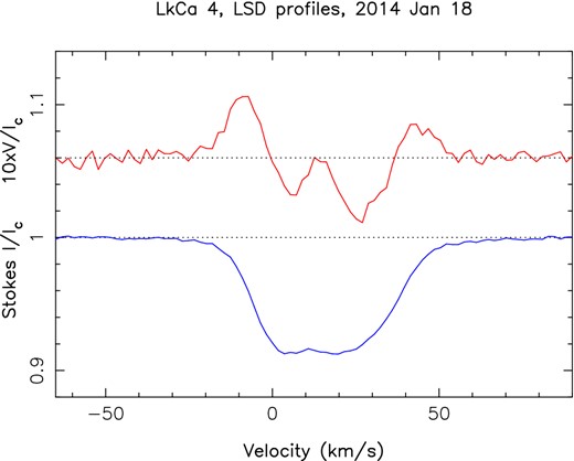
LSD circularly polarized (Stokes V) and unpolarized (Stokes I) profiles of LkCa 4 (top/red, bottom/blue curves, respectively) collected on 2014 January 18 (cycle 2.976). A clear and complex Zeeman signature (with a full amplitude of 1 per cent) is detected in the LSD Stokes V profile, in conjunction with the unpolarized line profile. The mean polarization profile is expanded by a factor of 10 and shifted upwards by 1.06 for display purposes.
Observed (open square and error bars) location of LkCa 4 in the HR diagram. The PMS evolutionary tracks and corresponding isochrones (Siess, Dufour & Forestini 2000) assume solar metallicity and include convective overshooting. The green line depicts where models predict PMS stars start developing their radiative core as they contract towards the MS.
Contemporaneous BVRJ photometric observations were also collected from the CrAO 1.25-m telescope between 2013 September and December, indicating that LkCa 4 was undergoing brightness modulations (with a period compatible with the rotation period of Grankin et al. 2008) of full amplitude 0.35 mag in V (see Table 2) – on the low side of what is reported for this star (with amplitudes in V fluctuations ranging from 0.35 to 0.79, Grankin et al. 2008). Again, this is clearly indicative of large spots at the surface of LkCa 4.
3 EVOLUTIONARY STATUS OF LKCA 4
LkCa 4 is a single star, showing no spectroscopic or imaging evidence for a companion (e.g. White & Ghez 2001; Kraus et al. 2011). Applying the automatic spectral classification tool especially developed in the context of MaPP and MaTYSSE, inspired from that of Valenti & Fischer (2005) and discussed in a previous paper (Donati et al. 2012), we find that the photospheric temperature and logarithmic gravity of LkCa 4 are, respectively, equal to |${T_{\rm eff}}=4100\pm 50$| K and |${\log g}=3.8\pm 0.1$| (with g in cgs units). This temperature estimate agrees well with that of Grankin (2013) derived from photometric colours, but is significantly larger than that obtained by Herczeg & Hillenbrand (2014) from fits to flux calibrated low-resolution spectra.1 In addition to being based on higher-resolution spectra and to providing a better match to photometry, our temperature estimate also has the advantage of being homogeneous with those derived in our previous studies of cTTSs (e.g. Donati et al. 2013), rendering internal comparisons simpler and more meaningful. From the B − V index expected at this temperature (equal to 1.20 ± 0.02; Pecaut & Mamajek 2013) and the averaged value measured for LkCa 4 (equal to ≃1.42; see Grankin et al. 2008, see also Table 2), we find that the amount of visual extinction AV that LkCa 4 is suffering is moderate, equal to 0.68 ± 0.15. Similarly, the visual bolometric correction expected for this temperature is found to be −1.00 ± 0.05 (Pecaut & Mamajek 2013).
Journal of contemporaneous CrAO multicolour photometric observations of LkCa 4 collected in late 2013, respectively, listing the UT date and Heliocentric Julian Date (HJD) of the observation, the measured V magnitude, B − V and V − RJ Johnson photometric colours, and the corresponding rotational phase (using again the ephemeris given by equation 1).
| Date | HJD | V | B − V | V − RJ | Phase |
|---|---|---|---|---|---|
| (2013) | (2456000+) | (mag) | |||
| Sep 01 | 537.5417 | 12.780 | 1.469 | 1.431 | 0.016 |
| Sep 11 | 547.5133 | 12.819 | 1.496 | 1.421 | 0.971 |
| Oct 11 | 577.5613 | 12.942 | 1.507 | 1.460 | 0.877 |
| Oct 27 | 593.5458 | 12.821 | 1.351 | 1.440 | 0.615 |
| Oct 29 | 595.5525 | 12.699 | 1.409 | 1.420 | 0.209 |
| Oct 30 | 596.5834 | 12.669 | 1.419 | 1.406 | 0.515 |
| Nov 08 | 605.5484 | 12.749 | 1.476 | 1.421 | 0.172 |
| Nov 09 | 606.5891 | 12.658 | 1.447 | 1.399 | 0.480 |
| Nov 10 | 607.4750 | 13.010 | 1.504 | 1.448 | 0.743 |
| Dec 03 | 630.4152 | 12.730 | 1.478 | 1.432 | 0.542 |
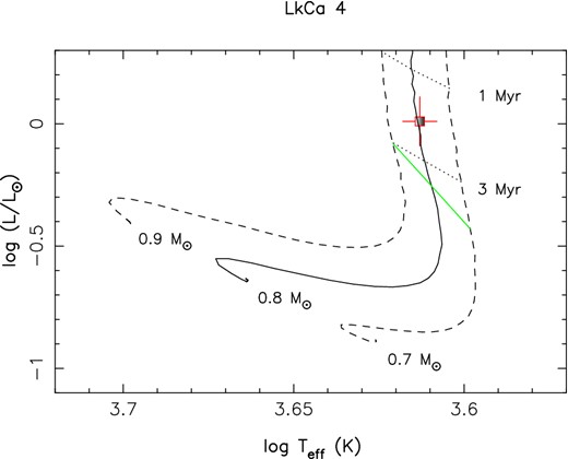
Accurate distances to young stars near LkCa 4 in Taurus measured with Very Long Base Interferometry (namely the wTTSs Hubble 4, HDE 283572 and the quadruple wTTSs system V773 Tau, Torres et al. 2007, 2012) are all consistent with an average distance of 130 pc to within better than 5 pc, implying a distance modulus of 5.57 ± 0.08 for LkCa 4 (provided it belongs to the same star formation complex). Assuming for LkCa 4 an unspotted V magnitude of 12.1 ± 0.2 (given the maximum V magnitude of 12.3 reported by Grankin et al. 2008, and taking into account a spot coverage of ≃20 per cent at maximum brightness, typical for active stars, see also Section 4), we finally obtain a bolometric magnitude of 4.85 ± 0.27, or equivalently a logarithmic luminosity (relative to the Sun) of −0.04 ± 0.11.
Considering that the rotation period of LkCa 4 is 3.374 d (Grankin et al. 2008) and that its line-of-sight-projected equatorial rotation velocity vsin i is 28.0 ± 0.5 km s−1 (see Section 4), we can infer that R⋆sin i = 1.87 ± 0.03 R⊙ where R⋆ and i, respectively, note the radius of LkCa 4 and the inclination of its rotation axis to the line of sight. Given our photospheric temperature estimate of |${T_{\rm eff}}=4100\pm 50$| K, we derive a minimum logarithmic luminosity (with respect to that of the Sun) of −0.05 ± 0.04. This clearly indicates that i is large, typically ranging from ≃60° (for our upper limit of ≃0.07 for the logarithmic luminosity) up to ≃90° (for the minimum logarithmic luminosity of −0.05).
In the forthcoming study, we adopt for LkCa 4 an intermediate inclination of i = 70°, corresponding to a relative logarithmic luminosity of 0.0 ± 0.1 and a radius of 2.0 ± 0.2 R⊙. Using the evolutionary models of Siess et al. (2000) (assuming solar metallicity and including convective overshooting), we obtain that LkCa 4 is a 0.79 ± 0.05 M⊙ star of age ≃2 Myr (see Fig. 2), indicating that this star is still fully convective and structurally similar to the prototypical cTTSs AA Tau and BP Tau. Our estimates are in reasonable agreement with those found in the refereed literature (e.g. Grankin 2013).
We finally report that Ca ii IRT lines of LkCa 4 feature core emission, with an average equivalent width of the emission core equal to ≃9 km s−1, i.e. very close to the amount expected from chromospheric emission for such PMS stars (e.g. Donati et al. 2013); similarly, the He iD3 line is barely visible (average equivalent width of ≃10 km s−1). In both cases, this is a reliable indication that LkCa 4 is no longer accreting material on its surface, thus further confirming its wTTS status in agreement with other recent studies (e.g. Gómez de Castro 2013). This makes LkCa 4 a very interesting target for probing a transition stage that is critical for our understanding of star and planet formation.
4 TOMOGRAPHIC MODELLING
In this section, we describe the application of our dedicated stellar-surface tomographic-imaging tool to our new spectropolarimetric data set. The software package we are using for this purpose is based on the principles of maximum-entropy image reconstruction, assuming that the observed variability is mainly caused by rotational modulation (with an added option for differential rotation). Since the initial release (Brown et al. 1991; Donati & Brown 1997), this package underwent several significant upgrades (e.g. Donati 2001; Donati et al. 2006b), the most recent one being its re-profiling to the specific needs of MaPP observations (Donati et al. 2010b). The reader is referred to these papers for more general details on the imaging method.
We use here this last version in a slightly modified configuration that allows a more accurate modelling of the MaTYSSE data. More specifically, the code is set up to invert (both automatically and simultaneously) time series of Stokes I and V LSD profiles into brightness and magnetic maps of the stellar surface. The reconstructed brightness map is now allowed to include not only cool regions (as before) but also bright plages as well – known to be participating to the activity of very active stars, especially those like LkCa 4 featuring extreme levels of photometric variability. This is achieved by allowing the reconstructed surface brightness (normalized to that of the photosphere) to vary both below and above 1, rather than being constrained to a ]0,1] interval, and by modifying accordingly the entropy associated with this image quantity.
While using sets of Stokes I, V, Q and U (rather than only I and V) profiles could in principle be useful to further constrain the imaging process and eliminate potential imaging artefacts (e.g. Donati 2001; Kochukhov & Piskunov 2002), it turns out to be unfeasible in practice for stars as faint as TTSs. Stokes Q and U Zeeman signatures are indeed much weaker than their Stokes V equivalents; moreover, they depend in a much stronger way on the actual Zeeman patterns of individual lines, making them far less suited to LSD-like multiline techniques without which they are basically impossible to detect. As a result and for a given amount of observing time, tomographic magnetic imaging of TTSs ends up being more efficient when applied to data sets limited to Stokes I and V profiles only, but featuring a phase coverage 3 times denser than if all Stokes profiles were recorded. Moreover, by making adequate prior assumptions on the magnetic topologies to be imaged (described as a low-order multipolar expansion), one can largely suppress most residual imaging artefacts even when only Stokes I and V profiles are used (e.g. Donati 2001).
The local Stokes I and V profiles used to compute the disc-integrated average photospheric LSD profile of LkCa 4 are synthesized using Unno-Rachkovsky's analytical solution to the equations of polarized radiative transfer in a Milne-Eddington model atmosphere, known to provide a reliable description (including magneto-optical effects) of how shapes of line profiles are distorted in the presence of magnetic fields (e.g. Landi degl'Innocenti & Landolfi 2004). The main parameters of this local profile are similar to those used in our previous studies, the wavelength, Doppler width, equivalent width and Landé factor being, respectively, set to 670 nm, 1.8 km s−1, 3.9 km s−1 and 1.2.
As part of the imaging process, we obtain accurate estimates for several parameters of LkCa 4. We find in particular that the average RV of LkCa 4 is 16.8 ± 0.1 km s−1 (more about this in Section 5) and that the vsin i is equal to 28 ± 0.5 km s−1.
4.1 Brightness and magnetic imaging
We show in Fig. 3 our set of Stokes I and V LSD profiles of LkCa 4 along with our fit to the data, and in Fig. 4 the corresponding brightness and magnetic maps that we reconstruct from fitting these data. The fit we obtain corresponds to a reduced chi-square equal to 1, starting from an initial value of over 50 (for a null magnetic field and an unspotted brightness map), which further stresses the quality of our data set and the high performance of our imaging code at modelling the observed modulation of LSD profiles (also obvious from Fig. 3). Given this, the large vsin i and the reasonably dense phase coverage, we can safely claim that no significant imaging artefacts nor biases are expected in the reconstructed maps.

Maximum-entropy fit (thin red line) to the observed (thick black line) Stokes I (right-hand panel) and Stokes V (left-hand panel) LSD photospheric profiles of LkCa 4 in 2014 January. Rotational cycles and 3σ error bars (for Stokes V profiles) are also shown next to each profile.
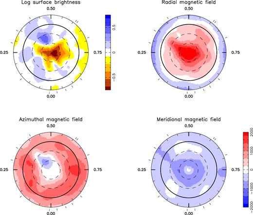
Maps of the logarithmic brightness (relative to the quiet photosphere, top left panel), radial (top right), azimuthal (bottom left) and meridional (bottom right) components of the magnetic field |${\boldsymbol B}$| at the surface of LkCa 4 in 2014 January. Magnetic fluxes are labelled in G. In all panels, the star is shown in flattened polar projection down to latitudes of −30°, with the equator depicted as a bold circle and parallels as dashed circles. Radial ticks around each plot indicate phases of observations.
The main feature of the reconstructed brightness map (see top left panel of Fig. 4) is a cool spot of complex shape near the visible pole, which directly reflects that the mean Stokes I LSD profile (not shown here, but resembling that at cycle 2.976, see Fig. 1 and left-hand panel of Fig. 3) features a flatter bottom than a pure rotation profile; although less dramatic for equator-on stars (with i ≥ 60°) than for pole-on ones (i ≤ 30°), this effect is nonetheless clearly detected in LkCa 4. This polar spot is found to be highly non-axisymmetric and rather complex in shape, with as much as three (and possibly up to five) different appendages towards lower latitudes, as evidenced by the large level of temporal variability in the unpolarized LSD profiles. The second most prominent feature of the brightness map is the warm plage reconstructed at phase 0.42 and at mid-latitudes, in which the local brightness rises up to ≃50 per cent above that of the mean quiet photosphere. Again, this directly reflects the very distorted shapes of Stokes I LSD profiles at phases in the range 0.25–0.60, i.e. when the plage is most visible to the observer and generates conspicuous absorption dips in spectral lines (at cycles, e.g. 3.288, 0.341, 2.413, see left-hand panel of Fig. 3). No similar fit to the data can be achieved if we force the code to reconstruct dark spots only at the surface of the star – an option implemented in our code and often used in Doppler imaging of cool stars to further constrain the inversion process with prior information on the image to be reconstructed. We therefore conclude that bright plages are clearly present at the surface of LkCa 4, rendering this imaging option mandatory for modelling MaTYSSE data. These two main surface features are found to cover altogether ≃25 per cent of the overall stellar surface. We stress that the photometric variations predicted by the reconstructed brightness maps are in very good agreement with the observations collected at CrAO (see Fig. 5), even though they were not recorded simultaneously with (but rather 1–4 months before) our spectropolarimetric data set (see Section 2); this suggests that the lifetime of brightness features at the surface of LkCa 4 is longer than a few months, fully compatible with previous conclusions from long-term photometric monitoring showing that light curves of LkCa 4 are remarkably stable in both shape and phase on time-scales of several years (see fig. 5 in Grankin et al. 2008).
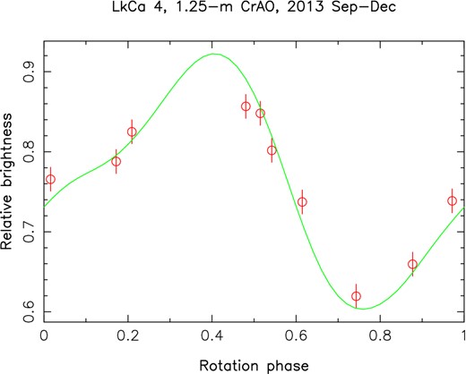
Brightness variations of LkCa 4 predicted from the tomographic modelling of Fig. 4 of our spectropolarimetric data set (green line), compared with contemporaneous photometric observations in the V band (red open circles and error bars) at the 1.25-m CrAO telescope.
The magnetic map shows a rather simple large-scale magnetic structure featuring two main components. The first one is a mostly axisymmetric poloidal field enclosing ≃70 per cent of the reconstructed magnetic energy; 94 per cent of the poloidal field energy gathers in spherical harmonics (SH) modes with m < ℓ/2 (ℓ and m denoting, respectively, the degrees and orders of the modes) while 86 per cent of it concentrates in the aligned dipole (ℓ = 1 and m = 0) mode. This poloidal component can be approximated with a dominant 1.6 kG dipole tilted at ≃10° to the line of sight (towards phase 0.75), with the addition of a 4 times weaker (≃0.4 kG) mostly axisymmetric octupolar component (roughly aligned with the dipole component), generating an intense radial field feature in excess of 2 kG at the visible pole of the star (see top right panel of Fig. 4) that coincides with the cool spot reconstructed in the brightness image. We also note that the elongated shape of this magnetic pole is similar to that of the cool polar spot.
The second main component of this large-scale field is a very significant, almost axisymmetric toroidal component showing up as an azimuthal field ring of ≃1 kG encircling the star at equatorial latitudes (see bottom left panel of Fig. 4). This feature directly reflects the nearly symmetric shape of the Stokes V LSD profiles (about the centre of the line profile) at most rotation phases (see right-hand panel of Fig. 3), known to be a clear signature of a prominent azimuthal field ring at the surface of the star. We also note the detection of an azimuthal field feature of opposite (i.e. clockwise) polarity in the immediate vicinity of (and possibly coincident with) the warm plage detected in the brightness image. SH expansions describing the reconstructed field presented in Fig. 4 are limited to terms with ℓ ≤ 10; only marginal changes to the solution are observed when increasing the maximum ℓ value from 10 to 15, demonstrating that most of the signal detected in Stokes V LSD profiles of LkCa 4 concentrates at large spatial scales.
We finally stress that reconstructing brightness and magnetic maps simultaneously from both Stokes I and V data (rather than separately from each other from either set of profiles) has no more than a small impact on our results; this is not altogether very surprising since magnetic and brightness imaging are largely decorrelated in low-mass stars with large vsin i's, where magnetic and brightness maps depend mostly on Stokes V and Stokes I data, respectively (rather than more or less equally on both). More specifically, virtually no change is observed in the brightness map when reconstructing it from Stokes I LSD profiles alone, magnetic fields having a much smaller impact than brightness features on disc-integrated line profiles for stars featuring high levels of rotational broadening. The non-simultaneous reconstruction of the brightness map has a larger, though still limited, impact on the magnetic map, reducing the strength of both dipole and octupole components (from 1.6 and 0.4 kG down to 1.4 and 0.2 kG, respectively) but leaving the overall topologies of the poloidal and toroidal fields (and in particular their orientation) unaffected. We nevertheless think that reconstructing both quantities from a simultaneous fit to Stokes I and V LSD profiles provides a more consistent and thus safer approach to the imaging of magnetic stars.
4.2 Surface differential rotation
In addition to showing Stokes I and V signatures detected at a very high confidence level, our spectropolarimetric data set includes observations spread over four rotation cycles of LkCa 4, making it well suited to look for signatures of differential rotation in the way outlined in several previous studies (e.g. Donati, Collier Cameron & Petit 2003; Donati et al. 2010a). Practically speaking, we achieve this by assuming that the rotation rate at the surface of the star is varying with latitude θ as |${\Omega _{\rm eq}}- {\rm d\Omega }\sin ^2 \theta$| where Ωeq is the rotation rate at the equator and dΩ the difference in rotation rate between the equator and the pole. The reconstruction code uses this law to compute, at each observing epoch, the amount by which each cell is shifted in longitude with respect to the meridian on which it is located at the selected reference epoch (chosen at mid-time in our observing run, i.e. cycle 2.0 in the present case). This allows the code to properly estimate the spectral contribution of each elementary region at the surface of the star to the synthetic disc-integrated Stokes I and V LSD profiles for given values of Ωeq and dΩ.
For each pair of Ωeq and dΩ within a meaningful range, we derive brightness and magnetic maps at a given information content as well as the corresponding reduced chi-squared |$\chi ^2_{\rm r}$| at which the modelled spectra fit the observations. We finally obtain |$\chi ^2_{\rm r}$| surfaces as a function of both Ωeq and dΩ, whose topology is directly indicative of whether differential rotation is detected, e.g. in the case of a convex surface featuring a clearly defined minimum. If so, this |$\chi ^2_{\rm r}$| surface can be used to estimate both Ωeq and dΩ and their respective error bars by determining the location of the minimum and the curvature radii of the |$\chi ^2_{\rm r}$| surface at this position. We usually achieve this by fitting a paraboloid to the |$\chi ^2_{\rm r}$| surface. This process has proved reliable for estimating surface differential rotation on various kinds of magnetic low-mass stars (e.g. Donati et al. 2003, 2010a).
The |$\chi ^2_{\rm r}$| surface associated with the brightness map features a clear minimum at |${\Omega _{\rm eq}}=1.868\pm 0.002$| rad d−1 and |${\rm d\Omega }=0.010\pm 0.006$| rad d−1 (see Fig. 6), whereas the magnetic map more or less repeats the same information but with ≃3 times larger error bars (|${\Omega _{\rm eq}}=1.865\pm 0.005$| rad d−1 and |${\rm d\Omega }=0.010\pm 0.020$| rad d−1). These values translate into rotation periods at the equator and pole of 3.364 ± 0.004 d and 3.382 ± 0.012 d, respectively, fully consistent with the time-dependent periods of photometric fluctuations reported in the literature for LkCa 4 (ranging from 3.367 to 3.387 d; Grankin et al. 2008) known to also probe surface differential rotation. This indicates that the surface differential rotation of LkCa 4 is small, much weaker in particular than that of the Sun (equal to ≃ 0.055 rad d−1) by typically 5.5 times; in fact, rotation at the surface of LkCa 4 is compatible with solid-body rotation within 1.7σ, with an average rotation period (of 3.369 ± 0.004 d) very close to the one found in the literature value (3.374 d) and used to phase our data (see equation 1). Brightness and magnetic maps computed assuming our estimate of surface differential rotation are virtually identical to those shown previously (see Fig. 4). The small amount of surface differential rotation is likely the reason behind the unusually long lifetime of brightness features on LkCa 4 reported above, as was already the case for the mid-M dwarf V374 Peg (Morin et al. 2008a).
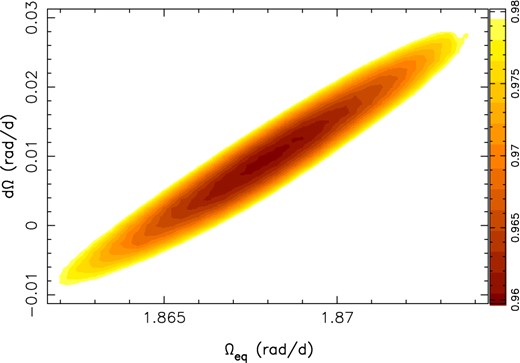
Variations of |$\chi ^2_{\rm r}$| as a function of Ωeq and dΩ, derived from the modelling of our Stokes I LSD profiles at constant information content. A clear and well-defined paraboloid is observed, with the outer colour contour tracing the 2.1 per cent increase in |$\chi ^2_{\rm r}$| that corresponds to a 3σ ellipse for both parameters as a pair.
5 FILTERING THE ACTIVITY JITTER
MaTYSSE also aims at detecting potential hJs orbiting wTTSs to quantitatively assess the likelihood of the disc migration scenario in which giant protoplanets form in outer accretion discs then migrate inwards until they fall into the central magnetospheric gaps of cTTSs. If this is indeed the case, one expects to find as many hJs as those found around MS stars, and possibly even much more, e.g. to account for those accreted by the central star at a later stage of evolution. However, detecting hJs around wTTSs is not obvious given their very large activity levels often generating RV jitters of a few km s−1, even at nIR wavelengths (e.g. Mahmud et al. 2011; Crockett et al. 2012). MaTYSSE therefore requires that we implement an efficient method for filtering out the RV jitter of wTTSs down to a level at which the RV signatures of hJs can be reliably detected.
We propose to achieve this RV filtering through the tomographic modelling of surface features from phase-resolved spectropolarimetric data sets such as that presented herein. As demonstrated in Fig. 7 in the particular case of LkCa 4, this technique is capable of reproducing activity-induced RV signals at an rms precision of 0.055 km s−1, i.e. 78 times smaller than the full amplitude of RV variations and less than twice the intrinsic RV precision / stability of ESPaDOnS for narrow-lined low-mass stars (of ≃0.03 km s−1). This RV precision is potentially enough to detect the presence of hJs, generating RV signatures with a typical semi-amplitude of up to several 0.1 km s−1, provided their orbital periods are not equal to the rotation period of the central star (or its harmonics). The technique we propose to implement in practice is to look at rms residuals in RV curves of wTTSs once filtered with the tomographic modelling outlined in Section 4. Whenever these residuals happen to be larger than 0.1 km s−1, we can suspect the presence of an hJ, and even more so if these residuals are found to vary periodically with time at a period other than the rotation period of the star and its aliases. Further confirmation can be obtained by achieving a second spectropolarimetric monitoring of the same star to validate the reality of the residual RV signal as well as its planetary origin. In the specific case of LkCa 4, the RV residuals exhibit an rms dispersion of only 0.055 km s−1 with no clear periodic signal with a semi-amplitude larger than 0.10 km s−1(see Fig. 7); we thus conclude that no evidence is found for the presence of an hJ.
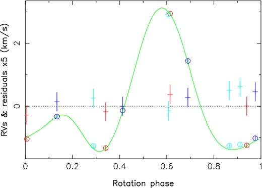
RV variations of LkCa 4 (in the stellar rest frame) as a function of rotation phase, as measured from our observations (open circles) and predicted by the tomographic maps of Fig. 4 (green line). RV residuals (expanded by a factor of 5 for clarity), are also shown (pluses) and exhibit an rms dispersion equal to 0.055 km s−1, i.e. 78 times smaller than the full amplitude of RV variations (of 4.3 km s−1). Red, dark blue and light blue symbols depict measurements secured at rotation cycles 0, 2 and 3, respectively (see Table 1). Given the highly distorted shapes of Stokes I LSD profiles (see Fig. 3), RV are estimated as the first-order moment of the LSD profile rather than through a Gaussian fit to it. All RV estimates and residuals are depicted with error bars of ±0.06 km s−1, estimated from our simulations and reflecting the noise level of our data (see text).
Preliminary simulations were carried out to confirm that the method we propose is feasible, and to obtain a first quantitative estimate of its performances. In these simulations, we compute a set of synthetic LSD profiles from the image of LkCa 4 we derived (see Fig. 4) covering a timespan and featuring a noise level similar to that of our observations; we add to these data a sinusoidal RV signal of semi-amplitude K and period Porb simulating the presence of an hJ in close-in circular orbit around the star. We then reconstruct a brightness image from this data set, use it to filter-out the RV curve from the activity jitter and look for periodic signals in the RV residuals. Results are promising and already confirm that the method we propose is valid; more specifically we find that:
the typical error bar on the RV residuals is 0.060 km s−1, i.e. fully compatible with the rms dispersion we measure, and mostly reflects the noise level in the data;
both K and Porb are recovered with reasonable accuracy when K is large enough, when Porb is not too close to the rotation period of the star Prot or to its first harmonic (0.5Prot) and when the phase coverage of the observations is reasonably even;
the 1σ error bar on the estimate of K depends both on the number of spectra and on the temporal sampling, decreasing from ≃0.03 km s−1 for a set of ≃16 evenly sampled spectra (the standard amount we aim at for MaTYSSE targets) to ≃0.02 km s−1 for twice as much – which should allow us to reliably detect hJs featuring K values of 0.15 and 0.10 km s−1, respectively;
the rms dispersion threshold on the RV residuals (of 0.10 km s−1) should be a reliable proxy that a planet is detected.
Of course, these preliminary results (see Fig. 8 for an illustration of a typical test) need to be confirmed and validated through a more extensive set of simulations. A forthcoming paper will be dedicated to this task; it will outline in particular the performances of our technique at detecting hJs around wTTSs and at estimating their orbital parameters (K and Porb), and will investigate thoroughly the impact of temporal sampling on these performances. For now, we can already conclude that the tomographic imaging method we described above is efficient at filtering out the activity jitter of wTTSs with extreme levels of activity like LkCa 4 and appears as a promising and powerful option for detecting hJs around young Suns.
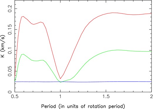
Semi-amplitude of the recovered RV signal, as a function of the size of the fake RV signal added to our synthetic data (simulating the presence of an hJ, see text) and of its period (the orbital period of the simulated hJ, in units of the rotation period of the star), for a simulated data set including 32 spectra evenly sampled over an interval of ≃3.5 rotation cycles. Red, green and blue curves, respectively, correspond to cases where the added RV signal has a semi-amplitude K of 0.2, 0.1 and 0.0 km s−1.
For each observing epoch, we are also able to determine the spot-corrected RV of the observed wTTS, i.e. the RV the star would show if no spots or plages were present at its surface. In the particular case of LkCa 4 in 2014 January, this spot-corrected RV is found to be 16.8 ± 0.1 km s−1. Looking at temporal variations of this quantity is yet another way of looking for giant planets orbiting close to very young Sun-like stars. This method requires multiple data sets such as that presented here, collected over a timespan of a few months, and is thus more time consuming than the approach outlined above; whenever applicable, it is nonetheless very complementary, offering in particular a better sensitivity to massive planets with longer orbital periods (of weeks rather than days).
6 SUMMARY AND DISCUSSION
This paper presents spectropolarimetric observations of the wTTS LkCa 4 collected with ESPaDOnS at the CFHT in 2014 January, and complemented by contemporaneous photometric observations from the 1.25-m telescope at CrAO, in the framework of the MaTYSSE international programme.
Applying our spectral classification tool to our CFHT data, we first find that LkCa 4 has a photospheric temperature of 4100 ± 50 K and a logarithmic gravity (in cgs units) of 3.8 ± 0.1; this suggests that LkCa 4 is a 0.79 ± 0.05 M⊙ star with a radius of 2.0 ± 0.2 R⊙ and a rotation axis viewed at an inclination angle of ≃70°. With an estimated age of ≃2 Myr, LkCa 4 is still fully convective. Emission in the Ca ii IRT and the He iD3 lines is weak, further confirming the non-accreting wTTS status of LkCa 4. In the HR diagram, it sits close to the prototypical cTTSs AA Tau and BP Tau, making LkCa 4 a key target for investigating how young Suns evolve once they dissipate their accretion discs and start spinning up towards the MS – a crucial transition for our understanding of star and planet formation. With a rotation period of 3.37 d, i.e. 2.4 times shorter than the typical 8-d rotation period of cTTSs in this range of age and mass, LkCa 4 is most likely in a process of rapid spin-up.
Using tomographic imaging on our phase-resolved spectropolarimetric data set, we recovered the brightness map and magnetic topology at the surface of LkCa 4 at the epoch of our observations. We find that LkCa 4 features a cool spot near the pole as well as a bright plage at intermediate latitudes, covering altogether ≃25 per cent of the overall stellar surface and generating large distortions in the unpolarized LSD profiles at nearly all rotation phases; the brightness map we derive is in good agreement with our contemporaneous photometric observations. We stress that including both spots and plages in the tomographic modelling is necessary to properly fit the observed spectra. We also find that this brightness distribution experiences very little latitudinal shear in the time-scale of four rotation cycles, implying that differential rotation at the surface of LkCa 4 is ≃5.5 times weaker than that of the Sun and compatible with solid-body rotation. We obtain that the large-scale magnetic field of LkCa 4 is strong and mainly axisymmetric, including both a ≃2 kG mostly dipolar poloidal field as well as a ≃1 kG toroidal component encircling the star at equatorial latitudes. The main radial field region is found to overlap with the cool polar spot in the brightness map; the bright plage is coincident with a region of negative (clockwise) azimuthal field.
Whereas the nearly axisymmetric kG poloidal magnetic field is very reminiscent of those of AA Tau and BP Tau (e.g. Donati et al. 2010b), the strong toroidal field component comes as a major surprise, as no such feature is observed on AA Tau nor BP Tau, nor on any of the other fully and mainly convective cTTSs more massive than 0.5 M⊙ observed to date (Donati et al. 2013). This feature is not observed either on low-mass MS stars with similar internal structures (Morin et al. 2008b). We note that the only other (and also fully convective and fairly young) wTTS for which magnetic maps are available in the refereed literature, namely V410 Tau, is also reported to host a significant toroidal field resembling that of LkCa 4 (Skelly et al. 2010), suggesting that what we report here for LkCa 4 is likely a common feature among young fully convective wTTSs rather than an isolated weirdness. This feature is unlikely to be related to the simple fact that wTTSs rotate significantly faster than cTTSs and to the potential differences this faster rotation could generate in the underlying dynamo processes; dynamos are indeed expected to be saturated in these stars and therefore to depend little on the stellar rotation rate. In fact, no such toroidal field structure is observed in fully convective M dwarfs, even for those with extreme rotation rates (Donati et al. 2006a; Morin et al. 2008a)
An alternative option could be that young fully convective wTTSs like LkCa 4 are triggering non-standard dynamos, as the potential result of an unusual internal rotation profile related to the rapid spin-up that wTTSs experience as they contract towards the MS, once the braking magnetic torque from the accretion disc no longer operates. However, angular momentum redistribution in convective layers is presumably occurring on time-scales much shorter than those associated with the dissipation of the disc or to the contraction of the star; this suggests that wTTSs are unlikely to feature internal rotation profiles that drastically differ from those of MS M dwarfs with similar internal structures and rotation rates, and thereby trigger exotic dynamos. Our observation that LkCa 4 exhibits no more than a weak surface shear, comparable to that of fully-convective M dwarfs (e.g. Morin et al. 2008a) and consistent with predictions of recent numerical simulations of fully convective stars (e.g. Browning 2008; Gastine, Duarte & Wicht 2012), brings further support in this direction and provides little help for explaining the surprising magnetic topology we unveiled. Hopefully, this issue will be clarified as MaTYSSE observations pile up and as results for stars of various masses, ages and rotation rates are obtained in a consistent way – allowing global trends and new clues to emerge.
Our tomographic technique is found to be efficient at modelling the activity jitter in RV curves of young active stars, at an rms RV precision of 0.055 km s−1 in the particular case of LkCa 4, i.e. 78 times smaller than the full amplitude of the RV jitter. This performance opens promising options for detecting hJs orbiting wTTSs through their periodic signatures in RV curves filtered out from the activity jitter. Preliminary simulations indicate that this technique is indeed capable of detecting hJs providing the semi-amplitude of their RV signature is larger than 0.10–0.15 km s−1 (depending on the number of spectra in the data set) and that the planet orbital period is not too close to the rotation period of the star (or its first harmonics); further simulations are needed to confirm and extend these conclusions, and will be presented in a forthcoming companion paper. We report no such evidence for an hJ in the particular case of LkCa 4; applying the same analysis to the whole MaTYSSE sample of about 35 wTTSs should allow us to obtain at least an upper limit on the fraction of wTTSs hosting hJs, and therefore to assess on observational grounds the standard mechanism proposed to explain the existence of hJs through disc migration at a very early stage of star / planet formation.
On a broader context and a longer time-scale, MaTYSSE studies will be extremely useful as science preparation for SPIRou – the nIR spectropolarimeter / high-precision velocimeter presently in construction for CFHT, for a first light in 2017. With its much higher sensitivity, SPIRou will be able to survey a far larger sample of wTTSs, thus expanding by typically an order of magnitude the pioneering work currently being carried out with MaTYSSE. Developing and validating activity-modelling and jitter-filtering techniques in the framework of MaTYSSE, such as those explored and described in the present paper, will be a key asset for the community as SPIRou comes on line and initiates its Legacy Survey of low-mass protostars.
This paper is based on observations obtained at the Canada–France–Hawaii Telescope (CFHT), operated by the National Research Council of Canada, the Institut National des Sciences de l'Univers of the Centre National de la Recherche Scientifique (INSU/CNRS) of France and the University of Hawaii. We thank the CFHT QSO team for the its great work and effort at collecting the high-quality MaTYSSE data presented in this paper. MaTYSSE is an international collaborative research programme involving experts from more than 10 different countries (France, Canada, Brazil, Taiwan, UK, Russia, Chile, USA, Switzerland, Portugal, China and Italy). We acknowledge funding from the LabEx OSUG@2020 that allowed purchasing the ProLine PL230 CCD imaging system installed on the 1.25-m telescope at CrAO. SGG acknowledges support from the Science & Technology Facilities Council (STFC) via an Ernest Rutherford Fellowship [ST/J003255/1]. SHPA acknowledges financial support from CNPq, CAPES and Fapemig. We finally thank the referee, Dr J. D. Landstreet, for his detailed reading of the manuscript and for suggestions to improve its overall clarity.
We suspect that this discrepancy is partly attributable to the different visual extinction they derived, and partly to the different spectral proxies used to estimate temperature (molecular features versus atomic lines in our case) rendering their technique presumably more sensitive to the presence of large cool spots at the surface of the star.
