


Abstract
We report the most comprehensive UBV(RI)C observations of the bright, radially pulsating field stars SW And, DH Peg, CU Com and DY Peg. Long-term variation has been found in the ultraviolet colour curves of SW And and DH Peg. We apply our photometric-hydrodynamic method to determine the fundamental parameters of these stars: metallicity, reddening, distance, mass, radius, equilibrium luminosity and effective temperature. Our method works well for SW And, CU Com and DY Peg. A very small mass 0.26 ± 0.04 M⊙ of SW And has been found. The fundamental parameters of CU Com are those of a normal double-mode RR Lyrae (RRd) star. DY Peg has been found to have paradoxical astrophysical parameters: the metallicity, mass and period are characteristic of a high-amplitude δ Sct star while the luminosity and radius place it in the group of RR Lyrae stars. DH Peg has been found to be peculiar: the definite instability in the colour curves towards ultraviolet; the dynamical variability of the atmosphere during the shocked phases suggests that the main assumptions of our photometric-hydrodynamic method, the quasi-static atmosphere approximation (QSAA) and the exclusive excitation of radial modes are probably not satisfied in this star. The fundamental parameters of all stars studied in this series of papers are summarized in tabular and graphical form.
1 INTRODUCTION
The first and second parts of this series of papers (Barcza 2010 and Barcza & Benkő 2012, hereafter Papers I and II) described a new method to determine the fundamental parameters of spherically pulsating stars with large amplitude, e.g. of RR Lyrae (hereafter RR) stars. The method is purely photometric: brightness and colour indices of atlas atmospheric models (Kurucz 1997) are compared with those from multicolour observations and the obtained physical parameters of the atmosphere are used in hydrodynamic equations for the pulsating atmosphere. Finally, the equations are solved for their parameters: stellar mass |${\cal M}_{\rm a}$| and distance d. The parameters like the reddening E(B − V) towards the star and atmospheric metallicity |$[M/\text{H}]$| are determined from shock-free phases. The variable physical parameters like the effective temperature Te(t), effective gravity ge(t) and stellar angular radius ϑ(t) = R(t)/d are obtained for all phases in the frame of quasi-static atmosphere approximation (QSAA), where R(t) is the radius of zero optical depth and t is the time. The method was applied for the RRab star SU Dra (Paper I) and after some technical refinements for the double-mode (DM) stars V500 Hya (= GSC 4868−0831) and V372 Ser (Paper II).
The main trend in the research of RR or other spherically pulsating stars with large amplitude is nowadays to use them as distance indicators and calibrating their astrophysical parameters (e.g. metallicity) from parameters like Fourier parameters of the light curve in an easily accessible broad photometric band. Simple fitting formulae are sought expressing the connection between data derived from the photometry in one band and the astrophysical parameters originating from involved theoretical considerations and computations. This is essentially a statistical approach.
We emphasize the astrophysical character of the method presented in this series of papers. We should like to understand better the response of the stellar atmosphere for the pulsational waves originating from the layers deeply below the atmosphere. We do it in the frame of our photometric-hydrodynamic method which is formulated in one spatial dimension as well as the present theories of stellar pulsation. We use the full colour information of a multicolour photometry (e.g. UBV(RI)C in this series of papers). The fundamental parameters are obtained without spectroscopic observations. It is crucial to use the information content of the ultraviolet part of the spectrum because reliable astrophysical parameters of these stars can only be obtained if the U band is included in the comparison of the observations and theoretical atmospheric models.
Our method is pioneering in making use of the laws of mass and momentum conservation in a pulsating atmosphere. It opened a completely new way to obtain simultaneously the mass and distance of the star.
This concluding paper of the series reports UBV(RI)C photometric observations and presents the new results for the fundamental parameters of the stars SW And, DH Peg, CU Com and DY Peg, respectively.
Sections 2 and 3 report the observations and the reductions. The results of the photometry are presented in Section 4. Metallicity, reddening derived from the colour indices of the shock-free epochs, the variable physical parameters, mass and distance to the stars and a brief insight in the dynamics of the atmosphere are given in Section 5. The main results (mass, distance, etc.) from Papers I and II are also included in the tables. The discussion and conclusions are given in Sections 6 and 7. These sections summarize the results of Papers I and II as well and the appraisal of our method.
2 THE OBSERVATIONS
A limitation in many previous photometric studies on these variables is that the light and colour curves were frequently obtained by folding observations over a long time (>103 × period Tifft 1964; Liu & Janes 1990) or one cycle was observed only (Paczyński 1965; Oja 2011).
We observed segments in the Johnson–Cousins UBV(RI)C light curves as long as they were allowed by the sky conditions and length of a night. Our light curves cover the period at least three times and we have the UBV(RI)C magnitudes for each observed star in more than 200 epochs distributed uniformly over the cycle. To our knowledge, the photometry reported here is the largest homogeneous observational material in the Johnson–Cousins system containing the U band. The wealth of this material allows us to discover some hitherto unknown details of the variability, e.g. cycle-to-cycle variations.
The observations were collected with the IAC801 telescope of the Teide Observatory and the 1 m RCC telescope mounted at Piszkéstető Mountain Station of the Konkoly Observatory of the Hungarian Academy of Sciences. The observational log is given in Table 1. The exposure times were 240, 60, 40, 10 and 10 s in U, B, V, RC and IC for the faintest star CU Com and 60, 40, 30, 8 and 8 s for DH Peg, respectively. A selection criterion of the target stars was that, according to the present-day classification scheme (Smith 1995), RRab-, RRc-, RRd- and SX Phe-type variables should be included in our study. Another selection criterion was that a comparison star of similar colour and check star(s) should be found within the CCD frame.
Log of the observations.
| HJD−2400000 | No. of frames | Telescope | |
|---|---|---|---|
| DY Peg, P = 0.072 926 492 d | |||
| 54345.3938–54345.7439 | 360 | IAC80 | |
| 54346.4689–54346.7162 | 435 | IAC80 | |
| 54347.4898–54347.7409 | 350 | IAC80 | |
| DH Peg, P = 0.255 510 37 d | |||
| 54349.4951–54349.7057 | 286 | IAC80 | |
| 54352.4426–54352.6952 | 410 | IAC80 | |
| 54354.3792–54354.6757 | 465 | IAC80 | |
| SW And, P = 0.442 266 d | |||
| 54350.4678–54350.7399 | 595 | IAC80 | |
| 54351.4689–54351.7354 | 535 | IAC80 | |
| 54353.4203–54353.7441 | 590 | IAC80 | |
| 54822.2272–54822.4665 | 320 | RCC | |
| 54829.2945–54829.4089 | 180 | RCC | |
| 54830.3834–54830.4302 | 75 | RCC | |
| 54831.3594–54831.4003 | 80 | RCC | |
| 54832.2465–54832.3726 | 205 | RCC | |
| CU Com, |$P_0=0.543\,9036\,\text{d}, P_1=0.405\,6130$| d | |||
| 54834.6136–54834.6923 | 50 | RCC | |
| 54871.6881–54871.7490a | 55 | IAC80 | |
| 54873.6045–54873.7612 | 135 | IAC80 | |
| 54874.5278–54874.7652a | 165 | IAC80 | |
| 56002.3537–56002.6375 | 270 | RCC | |
| 56003.3173–56003.5793 | 155 | RCC | |
| 56004.3384–56004.6196 | 235 | RCC | |
| 56005.4446–56005.6223 | 140 | RCC | |
| 56006.3127–56006.6300 | 285 | RCC | |
| 56007.3018–56007.6325 | 315 | RCC | |
| 56008.3011–56008.6224 | 310 | RCC | |
| 56018.4911–56018.5652 | 35 | RCC | |
| 56019.3204–56019.6266 | 280 | RCC | |
| 56020.3857–56020.6003 | 150 | RCC | |
| 56021.2945–56021.3516 | 60 | RCC | |
| 56022.4480–56022.5275 | 80 | RCC | |
aEpoch of the tie-in observations.
The source of the periods. DY Peg and CU Com: this work, DH Peg: Jones, Carney & Latham (1988), SW And: Liu & Janes (1989).
The comparison stars were GSC 1712−0984 (DY Peg), GSC 0565−1105 (DH Peg), GSC 1737−0809 (SW And) and GSC 1447−0968 (CU Com).
The check stars were GSC 1712−1246 (DY Peg), GSC 0565−1155 (DH Peg), GSC 1737−1139, GSC 1737−1194 (SW And) and GSC 1447−1184 (CU Com).
3 THE PHOTOMETRIC REDUCTION
The reduction of the frames was performed in the same way as described in Paper II. Standard iraf2 tasks were used and the details will not be repeated here.
The optical spectrum is sampled in U, B, V, RC and IC bands; therefore, it is of particular importance that the photometric system of the actual telescope and of the atlas models (the filters functions, the zero-points of the stellar magnitude scales) should be identical to avoid systematic errors in the derived atmospheric parameters. Therefore, heed must be given to transforming the instrumental magnitudes (u, b, v, r, i) to the standard UBV(RI)C ones. The constancy of the photometric constants of the telescope was verified by the check stars in order to obtain magnitudes of the best accuracy and sort out epochs when sky conditions became insufficient to a linear transformation between the instrumental and standard magnitudes. The u, b, v, r, i magnitudes were obtained in all frames from differential photometry with respect to the comparison star.
3.1 Tie-in to standard UBV(RI)C
The tie-in observations of CU Com were done under photometric quality sky conditions. The results are summarized in Table 2.
The result of the photometry in the field of CU Com.
| GSC 1447− | V | B − V | U − B | V − RC | V − IC |
|---|---|---|---|---|---|
| 0968 | 11.747 | 0.500 | 0.042 | 0.270 | 0.560 |
| 1551 | 10.889 | 0.485 | 0.100 | 0.296 | 0.588 |
| 1184 | 12.561 | 0.473 | 0.061 | 0.261 | 0.507 |
| 1247 | 14.090 | 0.781 | 0.561 | 0.448 | 0.894 |
| 1863 | 14.012 | 0.616 | 0.237 | 0.387 | 0.732 |
| 0898 | 11.586 | 0.992 | 1.008 | 0.665 | 1.254 |
The errors of V, B − V, etc. are 0.004, 0.006, 0.013, 0.009, 0.009 mag from the 12 observations of the field.
GSC 1447−1247 was observed by Clementini et al. (2000) in B, V, IC; their and our magnitudes agree within 1σ.
The photometric data.
| # SW And, folded V and colours, comp. star: GSC 1737−0968, | ||||||
| … | ||||||
| # phi, V, B − V, U − B, V − R, V − I, HJD−2400000 | ||||||
| 0.0019 | 9.165 | 0.247 | 0.033 | 0.152 | 0.293 | 54350.7311 |
| 0.0069 | 9.169 | 0.246 | 0.035 | 0.155 | 0.3 | 54350.7333 |
| 0.0119 | 9.183 | 0.244 | 0.031 | 0.162 | 0.303 | 54350.7355 |
| … | ||||||
The complete table is published in the online version as an attached file data_FundparRRL_III.txt.
During the observation of SW And, DH Peg and DY Peg with IAC80, the sky quality was good only for differential photometry. We made an attempt to tie-in observations (night HJD = 2454348); however, we do not give the results because the zero-points of the magnitude scales were obviously distorted by the slightly variable cirrus clouds over the night. To overcome this difficulty, we used the telescope constants from our previous observations with the telescope IAC80 on HJD − 2454200 = 45–51 (Benkő & Barcza 2009) to convert the instrumental magnitude differences Δu, Δb, … to international ΔU, ΔB, … ones. Finally, ΔU, ΔB, … were linearly interpolated to the epoch of V observation to obtain the colour curves for all frames reported in Table 1.
A similar procedure was applied for the observational results of SW And with the RCC telescope. The congruence of the light and colour curves of SW And from the observations with the telescopes IAC80 and RCC in the shock-free phases and the identity of |$m_X^{\rm (z.p.)}$| with that of IAC80 at the reduction for SW And and DY Peg indicate that our light and colour curves are of sufficient quality to use them for determining the atmospheric parameters of the stars.
However, the derived shifts of zero-points |$m_X^{\rm (z.p.)}$| from SW And and DY Peg do not result in a congruence of light and colour curves of DH Peg with those of Tifft (1964), Paczyński (1965) and Jones et al. (1988), especially in U − B. This is caused, most probably, by cycle-to-cycle changes in U − B mentioned by Tifft (1964) and Bookmeyer et al. (1977). This systematic variation remained hidden, because observations in the U band are not available in the necessary number (e.g. Paczyński 1965; Liu & Janes 1990; Oja 2011). Therefore, we fixed the zero-points for DH Peg in a manner to reach a coincidence with the mean values in Table 4: the corrections |$m_X^{\rm (comp)}+m_X^{\rm (z.p.)}=9.873,\: 0.283,\: 0.509,\: 0.331,\: 0.685$| were applied in equation (1) for X = V, U − B, B − V, V − RC, V − IC, respectively.
Averaged values of the observed stars from the n epochs of the observations.
| 〈V〉 | 〈U − B〉 | 〈B − V〉 | 〈V − RC〉 | 〈V − IC〉 | |
|---|---|---|---|---|---|
| SW Anda, n = 61, HJD-2444720 = 0, 1, 3, 4 | |||||
| 9.700 | 0.195 | 0.423 | 0.266 | 0.532 | |
| SW And, n = 344, HJD-2454350 = 0, 1, 3 | |||||
| 9.730 | 0.010 | 0.496 | 0.262 | 0.554 | |
| SW And, n = 172, HJD-2454830 = −8, −1, 0, 1, 2 | |||||
| 9.746 | −0.024 | 0.500 | 0.241 | 0.514 | |
| SU Drab, n = 228 | |||||
| 9.834 | 0.010 | 0.311 | 0.251 | 0.530 | |
| DH Peg, n = 250 | |||||
| 9.508c | 0.201 | 0.275 | 0.190 | 0.411 | |
| DY Peg, n = 229 | |||||
| 10.427 | 0.087 | 0.294 | 0.208 | 0.374 | |
| CU Com, n = 543 | |||||
| 13.313 | 0.056 | 0.350 | 0.196 | 0.427 | |
| V372 Serd, n = 529 | |||||
| 11.350 | 0.000 | 0.380 | 0.256 | 0.524 | |
| V500 Hyad, n = 280 | |||||
| 10.769 | −0.087 | 0.357 | 0.215 | 0.478 | |
The magnitude differences of the comparison and check stars were used in all fields to control the quality of the photometry at each epoch. The standard deviation σ of the differences indicates the average noise of the magnitudes of the variables at an epoch. Of course, it is the highest for the faintest check star GSC 1447−1184: σ(V) = 0.006, σ(B − V) = 0.007, σ(V − RC) = 0.009, σ(V − IC) = 0.011, σ(U − B) = 0.036 mag are for the whole set.3
4 RESULTS OF THE PHOTOMETRY
The photometric data (see Table 3) are published for all stars in electronic form.4 The magnitude averaged V and colour indices are given in Table 4. The light and colour curves are described in the following subsections for each star. Before using them for a determination of the fundamental parameters, we mention some observational results which are interesting in themselves.
4.1 SW And
Variability of the comparison star GSC 1737−0809 (=SAO 073957) was suspected by Liu & Janes (1989). Our observations do not support it; the magnitude differences with respect to the check stars GSC 1737−1194 and GSC 1737−1139 are identical within the observational error. If a variability exists, its time-scale must be over years. We used this star as a comparison star.
We observed 62–73 per cent of the full light curves on HJD-2454300 = 50, 51, 53, an ascending branch between HJD − 2454832 = 0.25–0.37 and four shorter segments (at decreasing or minimal brightness). The folded light and colour curves are plotted in Fig. 1.
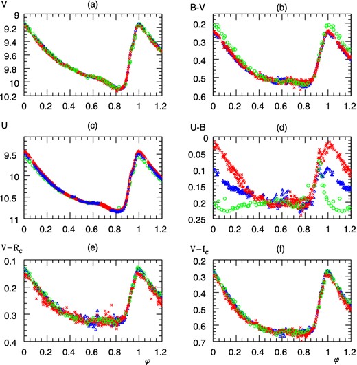
Light and colour curves of SW And as a function of phase φ. (Green) circles: 0 ≤ HJD − 2444720 ≤ 4 from the photometry of Liu & Janes (1989), (red) crosses: 0 ≤ HJD − 2454350 ≤ 3 (IAC80), (blue) triangles: 2 ≤ HJD − 2454820 ≤ 12 (RCC).
The large number of our observations pointed out a definite variation about 0.04 and 0.15 mag in B and U, respectively. It is clearly visible as a variation in U − B around the maximal brightness; the hump is present in all of our observed three ascending branches while it is missing in the colour curves of Liu & Janes (1989). This variation is plotted in Fig. 1(d). Therefore, when fixing the zero-point, our U − B colour indices could be shifted to the colour curve of Liu & Janes (1989) only in the shock-free phase interval φ = 0.4–0.92. An alignment is, however, impossible in the shocked intervals φ = 0.93–1, 0.0–0.4. A slight, much less pronounced difference is visible in the folded B − V colour curves as well (Fig. 1 b). The V phase diagram and the infrared colour indices are identical within the observational error if they are taken from our observations and from Liu & Janes (1989).
Balázs & Detre (1954) studied the long-term behaviour of the light curve of SW And and reported on a variable hump in the ascending branch and suspected a secondary (Blazhko?) period of 36.83 d. The hump is visible in our observations at φ ≈ 0.93 as a change of the slope in V as well as in U (Figs 1 a and c). The time coverage of our observations is not sufficient to confirm the secondary period of Balázs & Detre (1954) because the same phases Φ = 0.03 ± 0.05 belong to the epochs of Liu & Janes (1990) and Table 1 if they are folded with 36.83 d.
Although the amplitude variation of SW And is ≲ 0.02 mag in V (Barnes et al. 1988; Jones et al. 1992), this is at the noise limit of our observations, and the period must be long, the U and B observations allow us to confirm a change of the folded colour curves. The averaged colour dependence can be seen from the data in Table 4: B − V is redder and U − B is minimal at the maximal amplitude of the variation. SW And follows the rule: the maximal brightness in V and the minimal U − B coincide.
Liu & Janes (1990) ruled out a Blazhko-type modulation of the V light curve during the 3 d time-scale of their observations. Our observations confirm this finding; however, the data in Table 4 and Fig. 1 show clearly the long-term variation of the light curve which is more and more pronounced towards the ultraviolet part of the spectrum.
4.2 DH Peg
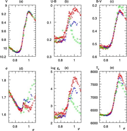
The phase diagrams of the check star GSC 0565−1155 and DH Peg are plotted in Fig. 2 with different symbols from the three nights. The differential magnitudes ΔX of GSC 0565−1155 were shifted in the magnitude range of Fig. 2. The magnitude differences of GSC 0565−1155 with respect to the comparison star GSC 0565−1105 are from the 236 frames: ΔV = −0.143 ± 0.011, Δ(B − V) = −0.435 ± 0.009, Δ(U − B) = −0.872 ± 0.012, Δ(V − RC) = −0.228 ± 0.009, Δ(V − IC) = −0.436 ± 0.008. The given small standard deviations show the good quality of the differential photometry within the frames. The following results of the differential photometry of DH Peg are independent from the uncertainty in the zero-points.
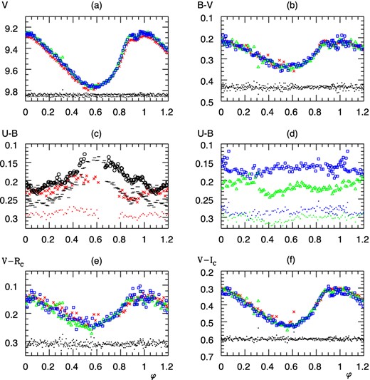
Folded magnitudes of DH Peg and the check star GSC 0565−1155. In all panels, (red) crosses: HJD=2454349, (green) triangles: HJD = 2454352, (blue) squares: HJD=2454354, dots: magnitudes of the check star GSC 0565−1155 calculated from the relative magnitudes with respect to GSC 0565−1105 and shifted in the panels. Short horizontal lines and circles in panel (c): U − B curves of Tifft (1964) and Paczyński (1965), respectively.
The hump before maximum is clearly visible in all bands. A variation of the zero-point and shape in Δ(U − B) ( ≲ 0.08 mag) is obvious from Figs 2(c) and (d). It is present to a lesser extent in Δ(B − V) ( ≲ 0.03 mag) as well (Fig. 2 b). This is essentially the variation of the U and B light curves amounting to about 0.08 and 0.03 mag, respectively. Its visibility is enhanced by looking at the colour indices. To demonstrate the variation in U − B, the curves on HJD − 2454300 = 49 and 52, 54 were plotted separately in Figs 2(c) and (d), respectively. The comparison of the three curves of DH Peg and that of GSC 0565−1155 shows clearly that the systematic difference in U − B of DH Peg is significant above the 3σ level.
A brightening about 0.05 mag of U − B is observable at φ ≈ 0.55 on 2454349 (Fig. 2 c). A similar, somewhat larger brightening (≈0.07 mag) is visible at this phase in the colour curves of Tifft (1964) and Paczyński (1965). This brightening is missing on HJD-2454400 = 52, 54 (Fig. 2 d); U − B remained approximately constant during the whole cycle as bright as on HJD = 2454349 at φ ≈ 0.55. A remarkable feature is that the maximal brightness in V is accompanied with maximal or approximately constant U − B; this is visible in the material of Tifft (1964) and Paczyński (1965), as well.
The three observed ascending branches in the near-infrared colours are identical within the scatter, while a minor systematic difference ( ≲ 0.03 mag) is observable in the descending branches. Because of the uncertainty of zero-points of the magnitudes, our amplitudes were compared with those of the published previous studies. The near-infrared amplitudes are identical to those from Jones et al. (1988). The amplitudes in B − V and U − B show differences of ≈0.02 and 0.06 mag, respectively.
4.3 CU Com
The folded light curves are not informative because of the presence of two periods with approximately the same amplitude; therefore, three characteristic segments are plotted in Fig. 3: a descending branch (A), a minimum (B) and a maximum (C). It is remarkable that U has a definite hump before maximum in segment (B) (Fig. 3c), and the slope of V shows a change here (Fig. 3a). This feature is present in the seven segments containing an ascending branch on HJD − 2456000 = 2, 3, 4, 6, 7, 19, 20. CU Com follows the rule: maximal brightness in V coincides with the minimal U − B.
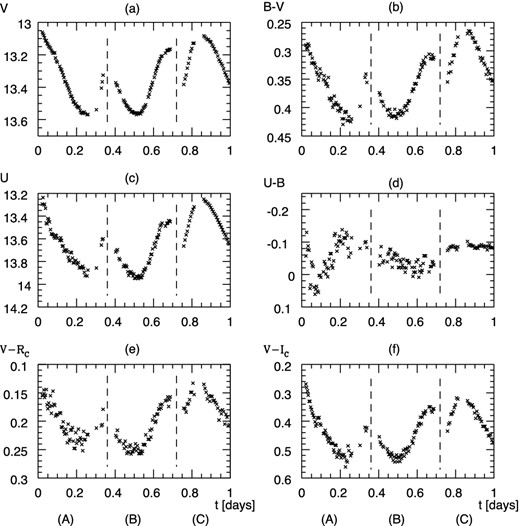
Three characteristic segments from the photometry of CU Com. To unify the segments in one figure, the following time shifts of the observed epochs were applied: t(A), (B), (C) = HJD − 2456008.28 (A), −2456001.95 (B) and −2454873.77 (C), respectively.
A Fourier analysis of the V light curve by the mufran program package (Kolláth 1990) yielded the periods |$P_0=f_0^{-1}=0.543\,9036\pm 0.000\,0030$| d and |$P_1=f_1^{-1}=0.405\,6130\pm 0.000\,0017$| d; the period ratio is P1/P0 = 0.745 744. The rest mean square of the residual is 0.016 mag after pre-whitening the frequencies if0, i = 1, 2, 3, 4, jf1, j = 1, 2, 3 and f0 ± f1 from the light curve. The frequencies f0 ± f1 could be definitely identified, that is, typical frequencies for an RRd star have been found. Small differences ΔP0 = −0.000 26 d and ΔP1 = −0.000 15 d of the periods can be seen in comparison with those from Clementini et al. (2000). This is equivalent to secular period changes |${\dot{P}_0}\approx -4.8\times 10^{-8}$| and |${\dot{P}_1}\approx -2.7\times 10^{-8}\;{d}^{-1}{\,d}$| which are by a factor O(103) larger than the values expected from stellar evolution theory and |$\dot{P}_0$| and |$\dot{P}_1$| found for the RRd star V372 Ser (Benkő & Barcza 2009). The period ratio P1/P0 = 0.745 658 (Clementini et al. 2000) changed ≈+ 1.15 × 10⁻⁴ over some 15 years.
4.4 DY Peg
The light and colour curves of DY Peg are plotted in Fig. 4. An evident feature is that the maximal brightness in V is accompanied with a maximal U − B. DY Peg behaves contrary to an RRab star having maximal V and minimal U − B simultaneously. A similar behaviour was observed at DH Peg. The other colour indices of DY Peg and RR stars show identical qualitative feature: the maximal brightness in V is accompanied with maximal brightness in B − V, V − RC and V − IC.
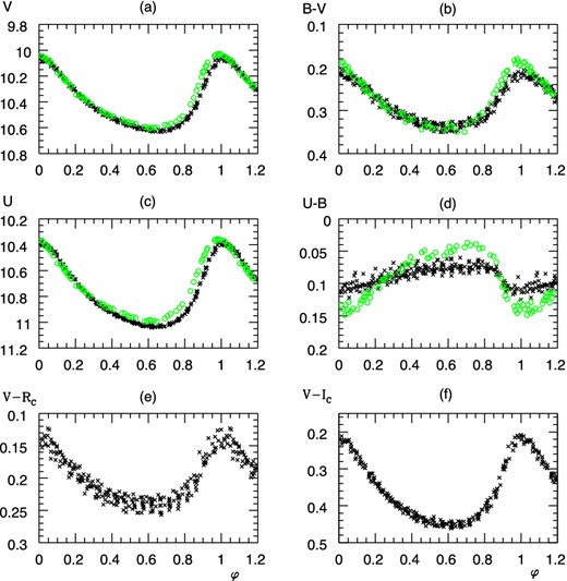
Folded light and colour curves of DY Peg. (Green) circles: from the UBV photometry of Oja (2011, HJD − 2450387 = 0.34–0.49), black crosses: from the IAC80 observations on HJD − 2454340 = 5, 6, 7.
We measured some 0.03 mag smaller amplitude of U − B in comparison with that of Oja (2011). This might be connected with the amplitude variation of the V light curve which has already been reported by numerous authors (e.g. Kozar 1980; Garrido & Rodríguez 1996; Pop, Liteanu & Moldovan 2003; Fu et al. 2009) who explained it by multiperiodic pulsation. A variability ≈0.04 mag was observed in V between two complete light curves taken with 12 d difference by Meylan et al. (1986).
The main pulsation frequency f0 = 13.712 438 d−1 (P = 0.072 926 492 d, see Table 1) and its four significant harmonics were detected by the mufran program package. After these frequencies were pre-whitened from the data, the spectrum of the residual still has some structure. A wide peak can be found at around 17.67 d−1 with the amplitude of ≈4 mmag. The resolution of the spectrum is very limited because of our short observing run; therefore, this peak is not significant (2σ). However, the position and amplitude of this peak agree well with the frequency of the first overtone pulsation reported in the cited literature. The short time span of our observations does not allow us to draw more quantitative conclusion on significant other period(s) and amplitudes belonging to them.
5 ASTROPHYSICAL PARAMETERS
The astrophysical parameters of the target stars were determined using the bbk package5 (Barcza 2011) as follows.
The metallicity |$[M/\text{H}]$| and the reddening E(B − V) towards the stars were determined by the minimization of the averaged errors of the effective temperature |$\overline{\Delta T_{\rm e}}$| and gravity |$\overline{\Delta \log g_{\rm e}}$| from the possible combinations of the colour indices (Barcza & Benkő 2009) using the photometry in the shock-free epochs. The upper limit of the search for E(B − V) was taken from the maps of the satellite Diffuse Interstellar Background Explorer (DIRBE; Schlegel, Finkbeiner & Davies 1998). The results are given in Table 5.
Metallicity, reddening, averaged surface gravity, effective temperature, angular radius of the stars and the standard deviation of the averaged quantities.
| |$[M/\text{H}]$| | E(B − V) | |$\overline{\log g_{\rm e}}$| | |$\overline{T_{\rm e}}$| | |$\overline{\vartheta \times 10^{11}}$| |
|---|---|---|---|---|
| (dex) | (mag) | (cm s−2) | (K) | (rad) |
| SW And, HJD-2444720 = 0, 1, 2, 3, 4 | ||||
| 0.02 | 2.60 ± 0.35 | 6676 ± 421 | 17.52 ± 0.68 | |
| HJD-2454350 = 0, 1, 3 | ||||
| 0.10 | 0.02 | 2.85 ± 0.63 | 6610 ± 428 | 17.31 ± 0.68 |
| HJD-2454830 = −8, −1, 0, 1, 2 | ||||
| 2.75 ± 0.44 | 6637 ± 393 | 17.53 ± 0.65 | ||
| SU Draa | ||||
| −1.60 | 0.015 | 2.72 ± 0.59 | 6743 ± 512 | 16.68 ± 0.91 |
| DH Peg | ||||
| −0.35 | 0.08b | 2.86 ± 0.43 | 7413 ± 312 | 16.90 ± 0.04 |
| DY Peg | ||||
| −0.05 | 0.0 | 3.41 ± 0.16 | 7157 ± 246 | 10.60 ± 0.19 |
| CU Com | ||||
| −2.20 | 0.02 | 3.09 ± 0.51 | 6925 ± 309 | 3.21 ± 0.12 |
| V372 Serc | ||||
| −0.53 | 0.003 | 3.24 ± 0.36 | 6713 ± 324 | 8.13 ± 0.16 |
| V500 Hyac | ||||
| −1.05 | 0.008 | 3.69 ± 0.50 | 6902 ± 261 | 10.17 ± 0.37 |
The following phase intervals were used in the folded colour curves to derive |$[M/\text{H}]$| and E(B − V).
SW And: 0.4 < φ < 0.8 (HJD − 2454300 = 50, 51, 53);
DH Peg: 0.1 < φ < 0.4 (HJD = 2454349);
DY Peg: 0.3 < φ < 0.8 (HJD = 2454300 = 45, 46, 47);
CU Com: 39 epochs were taken from the shock-free
intervals on HJD − 2454800 = 71, 73, 74.
The errors are |$\pm 0.10\:\mbox{dex}\text{ and}\:\pm 0.01\:\mbox{mag}$| (except for CU Com where it is ±0.20 dex), respectively.
aPaper I.
b Jones et al. (1988).
cPaper II.
The colour–colour diagrams of the atlas models (Kurucz 1997) were interpolated to the values of |$[M/\text{H}]$| and E(B − V) in Table 5, and they were used to determine ϑ, Te and ge as a function of phase. Their averaged values from our observations are given also in Table 5.
Next, the time-dependent quantities were introduced in the hydrodynamic equations which were solved for d and |${\cal M}_{\rm a}$| as described in Paper II. One point was added to the algorithm bbk: the lower limit |$d_{\rm min}=-g_{\rm e}(\varphi _1) {\ddot{\vartheta }}^{-1}(\varphi _1)$| of the search was introduced to exclude false roots of equation 4 of Paper II coming from terms ∝d−1; φ1 is the phase of minimal ge, |$\ddot{\vartheta }$| is the angular acceleration at the top of the atmosphere (in the reference frame of the observer) and the dot denotes a differentiation with respect to t. The results are summarized in Table 6. The following variable atmospheric parameters are plotted for each star in Figs 5– 9: angular radius ϑ(φ), effective gravity ge(φ), effective temperature Te(φ), barometric scaleheight for unit averaged molecular mass μ at the top of the atmosphere |$\mu h^{-1}_0(\varphi )={\cal R}T(R,\varphi )g^{-1}_{\rm e}$|, radius R(φ) and pulsational velocity v(φ) and |$\cal R$| is the universal gas constant.
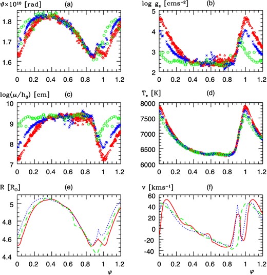
The variable parameters of SW And as a function of phase in absolute units. Panel (a): the angular radius ϑ(φ) = R(φ)d−1, panel (b): the effective gravity log ge(φ), panel (c): the barometric scaleheight for unit averaged molecular mass μ at the top of the atmosphere, |$h_0(\varphi )=g_{\rm e}/{\cal R}T(R,\varphi )$|, panel (d): effective temperature Te(φ). Panel (e): the radius of zero optical depth R(φ), (green) dashed line: radius variation integrated from the radial velocity of Liu & Janes (1989), panel (f): the velocity v(R, φ), the (green) dashed line vpuls(φ) was computed from vrad(φ) of Liu & Janes (1989) with |${\cal P}_p=1.32$|, vγ = −20.9 km s−1 in equation (3). Green circles in panels (a)–(d) and dashed (green) lines in panels (e), (f): folded from HJD − 2447100 = 20.57–23.86 (Liu & Janes 1989). Red triangles in panels (a)–(d) and (red) lines in panels (e), (f): folded from HJD − 2454300 = 50.4–53.8. Blue crosses in panels (a)–(d) and dotted (blue) lines in panels (e), (f): folded from |${\rm HJD}-2454800=22.2\text{--}32.37$|.
Zoomed characteristic parameters of SW And during the most compressed state of the atmosphere. Green circles: folded from HJD − 2447100 = 20.57–23.86 (Liu & Janes 1990), (red) triangles: folded from HJD − 2454300 = 50.5991–50.7399, (red) squares: folded from HJD − 2454300 = 51.4821–51.7024, (blue) crosses: folded from HJD − 2454832 = 0.2465–0.3726.
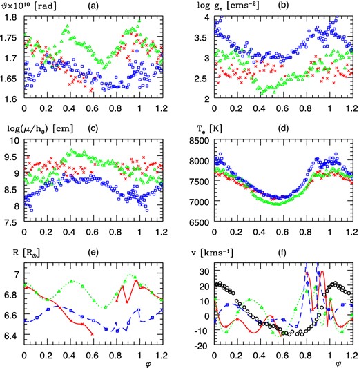
The variable parameters of DH Peg in absolute units. For the order of the panels, see Fig. 5. Red crosses, (green) triangles, (blue) squares: data from HJD-2454300 = 49, 52, 54, respectively. Red line, (green) dotted, (blue) dashed in panels (e), (f): HJD − 2454300 = 49, 52, 54, respectively. Black circles: pulsation velocity from Jones et al. (1988).

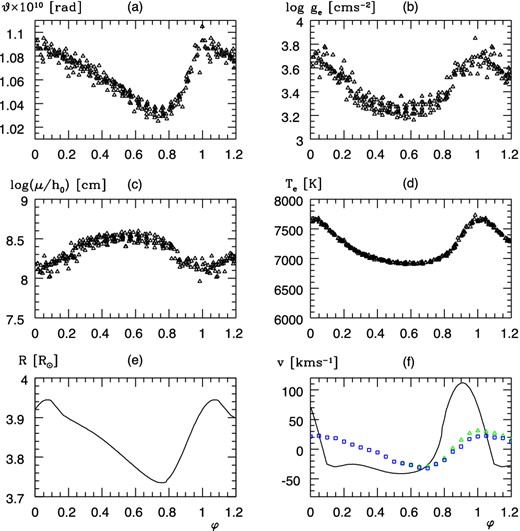
The variable parameters of DY Peg in absolute units. For the order of the panels, see Fig. 5. Green triangles and blue squares in panel (f): vpuls(φ) computed from the radial velocity curve of Meylan et al. (1986) and Wilson et al. (1998) by equation (3) with |${\cal P}_p=1.41$| and vγ = −25 km s−1.
|${\cal M}_{\rm a}d^{-2}$|, distance d of the observed stars, the averaged residual acceleration of the atmosphere in the epochs when the dynamical condition C(II) (Paper I) of QSAA is satisfied, mass, equilibrium luminosity and effective temperature, minimal and maximal radius, magnitude averaged absolute visual magnitude and averaged ‘static’ surface gravity.
| |${\cal M}_{\rm a}d^{-2}\times 10^7$| | d | |$\overline{a^{\rm (dyn)}}$| | |${\cal M}_{\rm a}$| | Leq | Teq | Rmin, Rmax | 〈MV〉 | gs | |
|---|---|---|---|---|---|---|---|---|---|
| (M⊙ pc−2) | (pc) | (m s−2) | (M⊙) | (L⊙) | (K) | (R⊙) | (mag) | (m s−2) | |
| SWAnda | 7.00 ± 0.76 | 626 ± 31 | 0.27 | 0.26 ± 0.04 | 39.8 ± 4 | 6644 | 4.51, 5.05 | 0.710 | 3.09 |
| SWAndb | 1.685 | 41.5 ± 4 | 6672 | 4.53, 5.06 | 0.68 | 3.02 | |||
| SWAndc | 41.8 ± 4 | 6690 | 4.44, 5.05 | 0.655 | |||||
| SU Drad | 663 ± 67 | 0.68 ± 0.03 | 45.9 ± 9.3 | 6813 | 4.46, 5.29 | 0.68 | 8.3 | ||
| DH Pege | 9.20 ± 0.32 | 893 ± 104 | −0.03 | 0.73 ± 0.09 | 123 ± 27 | 7464 | 6.40, 7.06 | 0.02 | 4.50 |
| DY Peg | 2.42 ± 0.27 | 817 ± 24 | 1.40 | 1.40 ± 0.24 | 34.6 ± 2.1 | 7177 | 3.74, 3.95 | 0.84 | 30.2 |
| CU Com | 1.28 ± 0.21 | 3059 ± 181 | 0.02 | 0.55 ± 0.03 | 39.0 ± 4.7 | 6942 | 3.95, 4.70 | 0.82 | 8.00 |
| V372 Ser f | 6.12 ± 0.31 | 964 ± 81 | 0.41 | 0.57 ± 0.10 | 21.9 ± 5.2 | 6722 | 4.07, 4.40 | 1.58 | 12.9 |
| V500 Hya f | 40.3 ± 6.7 | 467 ± 16 | 2.40 | 0.88 ± 0.06 | 8.97 ± 1.23 | 6924 | 1.97, 2.05 | 2.40 | 54.8 |
The estimated errors of |$[M/\text{H}]$|, Teq and 〈MV〉 are |$\pm 0.1\,\mbox{dex}, 25\mbox{ K}\text{ and } 0.25\mbox{ mag}$|, respectively; |$g_{\rm s}=G{\cal M}\overline{R}^{-2}$|.
aHJD−2454350 = 0, 1, 3.
bHJD−2454830 = −8, −1, 0, 1, 2, |${\cal M}_{\rm a}$|, d of a were used.
cHJD−2444720 = 0, 1, 3, 4, |${\cal M}_{\rm a}$|, d of a were used.
dPaper I.
eThe data were determined from the photometry on HJD = 2454349, see the text.
fPaper II.
The photometric condition C(I) of the QSAA (Paper I) is not satisfied at the phase of maximal compression of the atmosphere in any of the stars. Therefore, some (positive) correction to ge(φ), Te(φ) can be expected here; however, the qualitative features of the curves remain unchanged: their maximal values are at the maximal luminosity and brightness in V. This correction does not have an effect on |${\cal M}_{\rm a}$| and d because they are determined from shock-free phases. Nevertheless, an effect on ϑ(t) and, of course, on |${\dot{\vartheta }}$| and |${\ddot{\vartheta }}$| can be expected.
5.1 SW And
The metallicity |$[M/\text{H}]=+0.1\pm 0.1$| dex from our photometric minimization method and Teq = 6644 K agree well with |$[M/\text{H}]$| and Te derived from high-dispersion spectra (Nemec et al. 2013). Remarkable is the small mass |${\cal M}_{\rm a}=0.26\pm 0.04$| M⊙ (Table 6).
Two particular features are worth mentioning from Fig. 5. To show them clearly, the zoomed variation of V, U − B, B − V, ϑ, log ge and Te is plotted in Fig. 6 as a function of φ.
Two atmospheric shocks can be observed on the ascending branch separated at φ ≈ 0.95. The first one is in the interval 0.8 ≲ φ ≲ 0.95, this is the precursor shock (Smith 1995), it is identical in each epoch and a rapid expansion of the atmosphere starts. The ‘main’ shock, the occurrence of another rapid expansion at 0.95 ≲ φ ≲ 1.01, is very different: it was missing, strong and medium strong during the observations at HJD − 2444720 = 0–3, HJD − 2454350 = 0–3 and HJD − 2454820 = 2–12, respectively. This double structure of the shock is reflected by the rapid change of the velocity v(R, φ) in the interval 0.9 ≲ φ ≲ 1.1: the line and the dotted line in Fig. 5(f) have two almost identical maxima separated by the minimal v(R, φ ≈ 0.98) ≈ −20 km s−1, that is by a short contraction episode. The violation of QSAA is stronger in the main shock than in the first one.
In addition to the maxima of v(R, φ) at φ ≈ 0.9, 1.06, two weak humps are visible at φ ≈ 0.38, 0.55 in the velocity curves from HJD-2454350 = 0, 1, 3; the hump at φ ≈ 0.38 is not visible on HJD ≈ 2454800. The undulation at ϑ ≈ 0.55 is visible in the material of Liu & Janes (1990) as well. This latter might be the pre-precursor shock which was found in ϑ(φ) of the RRab star SU Dra (fig. 1 in Paper I).
It is obvious that the shock hitting the atmosphere is more of hydrodynamic than thermal nature: it is more pronounced in ge(∝ϱ−1gradp) than in Te; the increments are about 1 dex and 4 per cent, respectively, where |$\varrho (r)\text{ and } p(r)$| are the density and pressure in the atmosphere.
5.2 DH Peg
The 24 shock-free phase points 0.1 < φ < 0.4 on HJD = 2454349 were used in the minimization process. An equivocal result was found in the interval 0 ≤ E(B − V) ≤ 0.1; therefore, we adopt E(B − V) = 0.08 (Jones et al. 1988) derived from the photometry in the Walraven system (Lub 1979). E(B − V) = 0.08 yields |$[M/\text{H}]=-0.35\pm 0.1$| dex from the minimization process; we use this value of metallicity. The errors are |$\overline{\Delta T_{\rm e}}=17$| K and |$\overline{\Delta \log g_{\rm e}}=0.071$| in the minimum. This metallicity differs from |$[M/\text{H}]=-0.8$| dex obtained from a differential curve-of-growth analysis of DH Peg (Butler 1975); however, it is in good agreement with |$[M/\text{H}]=-0.42$| dex derived from the Preston index (Butler 1975). (We remark that adopting |$[M/\text{H}]=-0.8$| dex would result in the increase to |$\overline{\Delta T_{\rm e}}=24$| K and |$\overline{\Delta \log g_{\rm e}}=0.092$|.)
A preliminary analysis of the data by the bbk package revealed that the atmosphere of DH Peg was almost continuously in a shocked state in the time intervals HJD−2454300 = 52.4426–52.6952 and 54.3792–54.6752 as is obvious from Fig. 7 and from the averages 〈log ge〉 = 2.565, 2.640, 3.297, and 〈Te〉 = 7337, 7323, 7554 K on HJD − 2454300 = 49, 52, 54, respectively. Thus, we could use the 57 epochs of |$\rm {HJD}-2454349=0.6244\text{--}0.7057$| (phase intervals 0.0016 < φ < 0.5879 and 0.8005 < φ < 1.0) in the bbk package to determine the data in Table 6. The inclusion of the omitted epochs from HJD − 2454300 = 52, 54 would increase d, |${\cal M}_{\rm a}$|, Leq, R, shifting DH Peg in a range of these parameters which is characteristic rather of a Cepheid or semi-regular variable.
Remarkable peculiarities are revealed by Fig. 7.
The minimal and maximal radius are at |$\varphi \approx 0.7\text{ and }0.95$|, respectively, that is, too early with respect to the maximal |$\log g_{\rm e}\text{ and }T_{\rm e}$|. The phase dependence of the atmospheric kinematics of DH Peg is different in comparison to an RRab star, e.g. SW And.
The amplitude of log ge is small (<0.6) over a time-scale of 0.26 d (≈P). This is characteristic of high-amplitude δ Sct (HADS) or SX Phe stars. The overall amplitude in the whole interval HJD − 2454300 = [49, 54] is ≈1.5, but even this higher value is below the characteristic value ( ≳ 2) for a normal RR star.
On the other hand, the average |$\overline{\log g_{\rm e}(\varphi )}=2.86$|, Teq = 7464 K and gs ≈ 4.5 m s−2 place DH Peg among the RRc stars.
5.3 CU Com
|$[M/\text{H}]=-2.2$| dex for CU Com supports the appropriateness of our photometric method since it is identical with the value found by Clementini et al. (2000) from high-dispersion spectroscopy.
The variable atmospheric parameters of CU Com are very similar to those of an RRab star; the response of the atmosphere to the pulsation does not differ from that of an RRab star. The presence of the period of the first overtone with comparable amplitude of the fundamental mode produces only a more complicated variability of the motions because the maxima and minima of the governing factors ge, Te belonging to the two frequencies are sometimes added or attenuated. CU Com follows the rule of the RR stars mentioned in Section 4.4: it can be seen from Figs 3 and 8 that minimal radius, barometric scaleheight, maximal effective gravity and temperature coincide with the minimal V, U − B, etc. There exist time intervals – e.g. section (B) in Fig. 8 – when the atmosphere is shock-free, QSAA is a good approximation and the dynamical corrections are small: a(dyn) ≪ gs. The amplitude of log ge is ≳ 2 which is the characteristic value of an RRab star.
5.4 DY Peg
E(B − V) = 0.0 and |$[M/\text{H}]=-0.05$| dex were found; this almost-solar metallicity suggests that DY Peg is rather a HADS, not an SX Phe star, as was classified on the basis of |$[M/\text{H}]=-0.7$| dex (Andreasen 1983).
The following pattern can be seen from Figs 4 and 9: maximal R, ge, Te, ϑ and minimal |$h_0^{-1}$| appear simultaneously at the maximal brightness in V which is accompanied, paradoxically, with maximal U − B. This behaviour is different from the phase dependence at RRab stars; it is similar to that found at DH Peg. The average log ge = 3.41 is larger; its amplitude is small (≈0.6) compared to the typical values of an RRab star. This behaviour is explained qualitatively by the larger static gs =30.2 m s−2 which is an attenuating factor during the pulsation.
6 DISCUSSION
As mentioned in Section 3, the zero-points from the attempt of the tie-in observations had to be shifted in order to bring our colours in coincidence with those of Tifft (1964), Paczyński (1965), Liu & Janes (1989) and Oja (2011). The uncertainty of zero-points of magnitude scales, the only dim term in our photometry, could not produce the observed variation in the colour curves of SW And, DH Peg and DY Peg. The study of the colour curves, especially U − B, revealed that changes of the light curve having a small amplitude in V can be easily detected by extending observations in the ultraviolet colour.
The extensive multicolour observations including the U band and using the different pairs of colour indices of the UBV(RI)C photometry allow us to determine the main governing atmospheric parameters Te(φ), ge(φ) better than the hitherto applied methods based on a single colour index using one (more or less arbitrarily chosen) colour index for Te(φ) and another one for ge(φ) (e. g. Jones et al. 1988; Liu & Janes 1989). Our method enables us to obtain more thorough and consistent information on the dynamical changes in the atmosphere of stars pulsating in radial modes. The parameters |${\cal M}_{\rm a}$| and the distance d to the star are parameters in the hydrodynamic Euler equation for the pulsation of the stellar atmosphere. [This perception allows us to determine the parameters on the basis of an astrophysical background. The Euler equation is written in Euler formalism (Pringle & King 2007)]. This is a dynamical method; it is completely different in comparison with the Baade–Wesselink (BW) method which is essentially a kinematic method, yielding d as a main result. Other astrophysical methods, the theories of stellar evolution and pulsation, give masses |${\cal M}_{\rm ev}$|, |${\cal M}_{\rm puls}$| and luminosity, where d is a derived quantity from comparing the theoretical and observed luminosities.
The accuracies are 10 and 2–3 per cent for |${\cal M}_{\rm a}d^{-2}$| and ϑ(φ), respectively; the differentiation of ϑ with respect to time allows the determination of the angular velocity and the angular acceleration of the pulsating atmosphere in the reference frame of the observer. They are used in the hydrodynamic equation of motion in the stellar reference frame and permit to clear up the kinematics and dynamics of the pulsating atmosphere in more detail than it could be done if the uniform atmosphere approximation (UAA) was used (which was defined in Paper I and is used also in any BW analysis.)
Of course, the QSAA is assumed during the whole cycle of the pulsation. It can surely be regarded as a first approximation; however, considerable corrections to QSAA can be expected only in the shocked phases. They are beyond the scope of the present series of papers and they have negligible effect on the derived fundamental parameters because |${\cal M}_{\rm a}d^{-2}$| and d are determined from inverting the photometry in the shock-free phases, and the other key quantity ϑ is also taken from the shock-free phases.
Now we discuss the results and compare them with the parameters obtained from a BW analysis, and remarks are given on the results for the stars.
6.1 Comparison of d with trigonometric parallax data
An important test for the reliability of our new photometric-hydrodynamic method is offered if trigonometric parallax of the target stars is available.
Parallax π = 1.42 ± 0.16 mas was measured for SU Dra with the Fine Guidance Sensor of the Hubble Space Telescope (Benedict et al. 2011) yielding d = 704 ± 79 pc. This value is in perfect agreement with d = 663 ± 67 pc (Paper I) and d = 640 ± 77 pc from a BW analysis (Liu & Janes 1989).
The satellite Hipparcos (Perryman 1997) measured |$\pi =-0.04\pm 1.50,\; 0.15\pm 1.42,\; 0.36\pm 2.02\text{ and}\; 1.11\pm 1.15$| mas for SW And, DH Peg, DY Peg and SU Dra, respectively. The revised values are |$\pi =1.48\pm 1.21,\; -2.89\pm 1.71,\; -1.22\pm 1.60\text{ and}\; 0.20\pm 1.13$| mas (Van Leeuwen 2007). These values can be regarded as a null result. However, d = 470 ± 40 pc of DH Peg (Jones et al. 1988) and d = 250 ± 40 pc of DY Peg (Burki & Meylan 1986) from a BW analysis must probably be too small because they yield π = 2.1 and 4.0 mas for these stars. Parallaxes of these values could have been measured by Hipparcos.
6.2 Comparison of v(R, φ) with pulsation velocity derived from radial velocity observations
a constant (|$1.3 \lesssim {\cal P}_p \lesssim 1.4$|) or even a φ-dependent |${\cal P}_p$| is assumed (Marengo et al. 2002),
vrad(φ) is taken from a photometric correlation of template spectra of non-variable stars with the spectra of the RR star having a variable spectrum,
|$v_{\rm puls}=\dot{\vartheta }d$| is assumed, and
vγ is obtained from integrating vrad(φ) and equating the upward and downward motions.
The radial velocity is derived from the masking technique (e.g. CORAVEL; Liu & Janes 1990) or high-dispersion spectra in a limited interval of wavelength (e.g. Jones et al. 1992). It is integral of a depth-dependent velocity field where the weight function is not known. We note that neglecting the velocity gradient in the pulsating atmosphere, that is, taking |$v(R,\varphi )={\dot{\vartheta }}d$|, and assuming a constant |${\cal P}_p$| results in UAA. It is a first approximation which ought to be refined. This refinement has, however, never been discussed in the numerous papers dealing with the BW method, despite the indication of the considerable velocity gradient in the pulsating atmosphere (see e.g. Oke, Giver & Searle 1962).
In addition to the problem of the velocity gradient in a pulsating, compressible stellar atmosphere, a practical problem of the BW study is the strong dependence of the error Δd/d on the error Δvγ discussed in Gautschy (1987) and Paper I. To determine vγ, a way consistent with equation (3) would be to select the phases φ0 when vpuls(φ0) = 0 and then vrad(φ0) = vγ. This is, however, not free of problems as can be demonstrated by looking at panel (f) of Figs 5, 7 and 9, because v(R, φ) has a complex structure and there exists a considerable phase lag between vpuls(φ) by equation (3) and |$v(R,\varphi )={\dot{\vartheta }}(\varphi )d+\cdots$|, that is vpuls(φ) and v(R, φ) are not comparable quantities. Smoothing the curves, adding an arbitrary phase lag vrad(φ + δφ), |$\delta \varphi \not=0$| and neglecting the additional terms of v(R, φ) can formally solve the problem; however, it cannot be motivated astrophysically. Qualitatively, it is obvious that the phase lag between the two curves is a consequence of the neglected velocity gradient in the expanding–contracting atmosphere.
The details of the problem can be visualized by the curves of SW And (Figs 5e and f.) The value of the phase lag δφ depends upon whether
R(φ) and 〈R〉 + ΔR or
v(R, φ ≈ 0.92) and vpuls(φ) or
v(R, φ ≈ 1.05) and vpuls(φ)
are brought to coincidence. The radius displacements 〈R〉 + ΔR(φ) calculated from equation (4) are plotted in Fig. 5(e) with 〈R〉 = 4.78 R⊙ and δφ = 0. The double peak of v(R, φ) is not visible in vpuls(φ) at all, perhaps because of the scarce sampling of vrad(φ) (Fig. 5 f). The panels demonstrate that there is an uncertain phase lag (|δφ| ≲ 0.1). The fine structure of R(φ) cannot be reproduced by the integration of the radial velocity if equations (3) and (4) are used. Reliable R(φ) could only be obtained if a better solution of equation (2) were applied than equation (3).
The motion of the atmosphere is derived in this series of papers from |$d, {\cal M}_{\rm a}$|, ϑ(t), Te(t), log ge(t) in absolute units. It is compared with the observed radial velocity data of SW And, DH Peg and DY Peg in panels (f) of Figs 5, 7 and 9. The difference between vpuls(φ) and v(R, φ) can partially be explained by the simplifications involved in a BW analysis and, additionally, by the difference between the characteristic time of a multicolour observation ( ≲ 3 min) and the longer exposure time to take a spectrum. The scanty sampling has a smoothing effect, e.g. the complex structure of R(φ) of DH Peg cannot be explored by numerically integrating vpuls(t) sampled in the interval 10–30 min.
These considerations substantiate why we trust better in the distances from the present study if there is a significant difference between them and those from a BW analysis.
6.3 Remarks on the observed stars
Fig. 10 is a plot of some characteristic results given in Tables 5 and 6. It gives an impression on the diversity of the physical parameters of the target stars which form a more or less uniform group of radially pulsating field stars if they are classified by periods and amplitudes in one broad optical band.
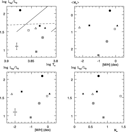
Luminosity–effective temperature, de-reddened visual absolute magnitude–metallicity, luminosity–metallicity and mass–luminosity diagrams of the observed stars. Filled circle: DH Peg, square: DY Peg, triangle: CU Com, filled square: SU Dra, filled triangle: SW And, circle with cross: V372 Ser, square with cross: V500 Hya. The estimated errors are plotted in the lower-left part of the left-hand panels. Lines in the upper-left panel: blue and red edge of the instability strip, dashed line: zero-age horizontal branch of M3 (Silva Aguierre et al. 2008).
The upper-left panel in Fig. 10 shows a plot of log Teq versus log Leq, a Hertzsprung–Russell diagram in terms of absolute astrophysical units showing a part of the instability strip. It is obvious that SW And, SU Dra, CU Com and DY Peg form a group (regular RR stars), while DH Peg is well above the horizontal branch formed by this group. V500 Hya is at the position expected for an SX Phe star; V372 Ser is at halfway between SX Phe and RR stars. This region was not explored by detailed hydrodynamic calculations; however, fig. 3 of Szabó, Kolláth & Buchler (2004) indicates the possibility of stable DM pulsation towards lower luminosities.
6.3.1 SW And
Significant differences have been found in the photometric and physical parameters on HJD − 2444720 = 0–3, HJD − 2454350 = 0–3 and HJD − 2454820 = 2–12: Leq = 41.8, 39.8 and 41.5 L⊙; Teq = 6690, 6644 and 6672 K; 〈MV〉 = 0.66, 0.71 and 0.68 mag (see Tables 4, 5 and 6). These variations confirm that P in Table 1 is not the sole period in the atmospheric pulsation.
SW And follows the rule that minimal radius, barometric scaleheight and maximal Te, ge belong to maximal brightness in V and minimal U − B (Figs 1 and 5); this is common in RRab stars.
The derived very low mass |${\cal M}_{\rm a}=0.26$| M⊙ is surprising. It was obtained from a background provided by theoretical model atmospheres and some hydrodynamics, not using the theory of pulsation and evolution of RR stars (Smith 1995). It is much lower than the canonical value ≈0.6 M⊙ of an RRab star (Liu & Janes 1989; Jones et al. 1992) or ≈0.5 M⊙ from the empirical Fourier fitting technique for metal-rich RR stars (Nemec et al. 2011). It is a serious challenge to the theories of stellar pulsation and evolution.
We remark that the mass of an RR-like star in the eclipsing binary system OGLE-BLG-RRLYR-02792 was found previously to be 0.26 ± 0.015 M⊙ (Pietrzyński et al. 2012) and has been substantiated by some theoretical considerations (Smolec et al. 2013). This favours the adoption of our anomalous mass value. Common features of SW And with OGLE-BLG-RRLYR-02792 are the bump in the middle of the ascending branch, and the similar luminosity and effective temperature Leq ≈ 39 L⊙, Teq ≈ 6664 K. [Smolec et al. (2013) found them as Leq ≈ 33 L⊙ and Teq ≈ 6970 K.]
The distances |$d=511\pm 56\text{ and}\; 481\pm 33$| pc were adopted by Liu & Janes (1989) and Jones et al. (1992), respectively; these are some 20 per cent smaller than our d = 626 ± 31 pc. The main argument to accept our larger distance to SW And is that |${\cal M}_{\rm a}d^{-2}=(7.00\pm 0.76)\times 10^{-7}$| (Table 6) was determined from the shock-free state of the atmosphere when the QSAA is expected to be a reliable approximation on an astrophysical basis. The value of |${\cal M}_{\rm a}d^{-2}$| is fairly firm central point in our theory. An adoption of the distances |$d=511\text{ and } 481$| pc would reduce the mass |${\cal M}_{\rm a}$| to a more anomalous low value ≲ 0.17 M⊙.
The difference between d = 511 and 481 pc can be attributed to the difference between vγ = −20.9 and −19.2 km s−1 in Liu & Janes (1989) and Jones et al. (1992), respectively, because an error 1 km s−1 of vγ results in an error Δd/d ≈ 0.1 (Gautschy 1987; Paper I). The uncertainty of vγ is obvious: vpuls(φ) ≈ 0 at φ = 0.4 ± 0.01 and 0.3 ± 0.01 from the IAC80 and RCC observations, respectively. The interpolated centre-of-mass velocities are vrad = −21 ± 1 and −28 ± 1 km s−1 (≈vγ!) from the observations of Liu & Janes (1989). The change of vγ from −21 to −28 km s−1 within 480 d might even be an indication for the binarity of SW And supported by the anomalous |${\cal M}_{\rm a}=0.26$| M⊙. Or more likely, it is an artefact yielded by the use of equation (3).
The differences in 〈R〉 = 4.36, 4.16 R⊙ (Liu & Janes 1989, Jones et al. 1992) and 4.78 R⊙ (Table 6), respectively, originate mainly from the different values of d. The derived photometric angular diameters of SW And do not differ significantly in the three studies.
6.3.2 DH Peg
The instability in (U − B)(φ) of DH Peg is known from previous observations and this seems to be a common feature of RRc stars (Tifft 1964). Our observations confirm the instability. The presence of other frequencies in RRc stars (Moskalik 2013) with increasing amplitude towards the ultraviolet could be a natural explanation of the non-repetitive character of the colour curves towards the ultraviolet and of the larger scatter in the descending branch of the near-infrared colour curves. Like at SW And, the observation and analysis of the ultraviolet part of the spectrum have led to a more detailed picture on the pulsation properties. The time span of our observations is short to draw a more definite conclusion.
The ambiguity |$[M/\text{H}]=-0.35\: \mbox{or} \: -0.8$| dex for DH Peg could have been caused by the long-term variation of the light curve and the breakdown of QSAA for the rapidly and intensively changing atmospheric conditions. A binning of non-coherent zero-points in our differential photometry seems to be an unreal possibility. Eventual adoption of |$[M/\text{H}]=-0.8$| dex would not result in a considerable change of the anomalous parameters in Table 6, but the decrease of 30 to 21 pairs of colour indices giving a solution for Te and log ge speaks strongly against |$[M/\text{H}]=-0.8$| dex.
Over a time interval of a few pulsation cycles, the large and systematic difference of the physical parameters, that is, approximately 1 dex difference in log ge and barometric scaleheight |$h_0^{-1}$|, and the complex structure of R(φ) and v(R, φ) suggest that periodic or stochastic variations are present in the atmosphere in addition to the period P in Table 1.
Furthermore, the violation of the assumptions involved in the QSAA and eventual excitation of non-radial mode(s) with large amplitude can also be a distorting factor for the derived fundamental parameters because our simplified (spherically symmetric) hydrodynamic model is not able to describe this type of the atmospheric pulsation. The large value of the dynamical correction term (|a(dyn)| ≳ ge) during the whole observed phases on HJD = 2454354 substantiates this conjecture, e.g. 〈log ge〉 ≈ 3.3 was during this period, some 0.6 dex higher than on HJD = 2454349. Large deviation from spherical symmetry would modify the colours compared to those of the atlas models.
Some cautiousness is appropriate in connection with the fundamental parameters of DH Peg derived by Jones et al. (1988) from the BW analysis. Their distance, and consequently their luminosity and 〈R〉, differs significantly from the values in Table 6. The upper and lower limits of the photometric angular radius are in good agreement with ours; however, there is a systematic difference in their ϑ(φ) derived from the different colour combinations and the cycle-to-cycle variations over a few pulsation periods are ignored. Finally, they select one colour index to determine ϑ(φ) without an attempt to reconcile the values from the different colour indices by taking into account the effect of the variable log ge(φ). The upper and lower limits originating from two different colour indices 6800 < Te(φ) < 7800 K are in coincidence with our values plotted in Fig. 7. However, the problem of selecting one colour index reducing the upper or increasing the above lower limits is again not solved.
The Jones et al. (1988) 470 ± 40 pc distance could reduce the luminosity to 34.1 L⊙, and the minimal and maximal radius to [3.37,3.72] R⊙. However, the complexity and the amplitude of v(R, φ) cannot be reconciled with the rather smooth vpuls(φ) (circles in Fig. 7 e) derived from observed radial velocities by equation (3). Furthermore, a large phase lag (Δφ ≈ −0.17) is necessary to bring the maxima of the two curves in coincidence. The null result of the Hipparcos parallax suggests larger d.
The following dilemma has emerged from the results. DH Peg is either an anomalous RR star with anomalous luminosity Leq ≈ 130 L⊙ and radius R ≈ 7 R⊙ exceeding the canonical values (Smith 1995) or it is a low-mass Cepheid with gs, Te exceeding the canonical values 0.01 ≲ gs ≲ 1 m s− 2, Te ≈ 5600 K (Marengo et al. 2002). Some cautiousness is appropriate concerning the row DH Peg in Table 6; however, our numerous attempts to revise them closer to the canonical values of RR stars could not lead to more conventional values. We think that a natural resolution of the dilemma is that the conditions C(I) and C(II) of QSAA are not satisfied in DH Peg.
6.3.3 CU Com
CU Com has a Galactic height ≈3 kpc and has a very low metallicity |$[M/\text{H}]=-2.2$| dex. These data show that CU Com might be a member of the outer halo population (Caroll et al. 2007). Its mass, radius, Leq, Teq and gs agree well with the canonical values for RRd stars. The mass 0.55 ± 0.03 M⊙ (Table 6) differs from the pulsation mass 0.830 ± 0.005 derived from a (several times revised) Petersen diagram (Clementini et al. 2000).
6.3.4 DY Peg
The conditions C(I) and C(II) (Paper I) are satisfied in all phases of DY Peg. The rapid change of the atmospheric parameters during the very short period was not found to be a hindrance to determine the astrophysical parameters. This demonstrates that our method is robust and works well for all types of radially pulsating stars with large amplitude.
The scatter of ϑ(φ), log ge(φ), h0(φ) and Te(φ) is a consequence of folding the photometry with the main period P = 0.072 926 492 d. The noise from probable other frequency mentioned in Section 4.4 and the non-photometric quality of the sky cannot be separated by folding.
The distance d = 250 pc from the BW analysis (Burki & Meylan 1986) would yield Leq ≈ 3.2 L⊙, 〈R〉 = 1.17 R⊙ and |${\cal M}_{\rm a}=2.42\times 10^{-7}\times 250^2 =0.13$| M⊙. These values are in contradiction with the present knowledge on HADS or SX Phe stars. A distance below 500 pc can be excluded on this basis. Application of an arbitrary phase lag Δφ = −0.12 in Fig. 9(f) could result in better agreement of v(R, φ) (calculated as given in Paper II) and vpuls(φ) calculated from the radial velocities (Meylan et al. 1986; Wils 2006) by equation (3). The presence of the phase lag and the uncertain value of vγ might be responsible for the very small d obtained from the BW analysis.
|${\cal M}_{\rm a}=1.40\,{\text{M}}_{\odot }$|, gs = 30.2 m s−2 and |$[M/\text{H}]=-0.05$| dex are characteristic of a HADS star. It is a paradoxical situation that Leq = 34.6 L⊙, 〈R〉 = 3.85 R⊙ and the position in Fig. 10 place DY Peg among the RR stars, but its short period P = 0.072 926 492 d is approximately one third of the period of the RRc stars with shortest period. The short period is the strongest argument against being an RR star.
7 CONCLUSIONS
The most comprehensive UBV(RIC) photometry and its interpretation using atlas atmospheric models have been reported in this series of papers for the field stars SU Dra, V500 Hya, V372 Ser, SW And, DH Peg, CU Com and DY Peg. The results could be obtained only by simultaneous multicolour observations; including an ultraviolet band is important! The interpretation has been done by simplified hydrodynamics using the mass and momentum conservation, that is by the continuity and Euler equations in Euler formalism (in the spherical reference system of the star). These laws were applied first time in the study of pulsating stars; their application belongs to the essence of our method. This method is pioneer in using a mixture of photometry and theory of stellar atmospheres.
The new method has rendered possible to determine the mass, distance and the better classification of radially pulsating stars. This could not be done merely by analysing frequencies or properties and parameters of light curves in a single (easily available) broad optical band. As a by-product, the method offers a better insight into the motion and dynamics of a pulsating stellar atmosphere.
The results and the physical parameters of the stars have been summarized in tabular form (Tables 4–6), and snapshots have been given about the variable atmospheric parameters.
Conclusions from the photometry. The U observations and the colour curves U − B have revealed a new complexity of the variability and have rendered possible to discover or confirm the unstable character of the light curve of SW And, DH Peg, and to a lesser extent in DY Peg. These findings suggest that either additional frequencies or some stochastic phenomena are present in the atmospheric response to the pulsation emerging from the sub-atmospheric layers. This result is a challenge to further theoretical investigations concerning pulsation and evolution theory.
Method of interpreting the photometry. The UBV(RI)C observations were interpreted by the atlas atmospheric models by comparing the theoretically calculated colours and colour indices (Kurucz 1997) with the observed ones. QSAA was assumed in all phases. All colour indices were used. It has been demonstrated that the use of one, more or less arbitrarily chosen, colour index for Te and another one for ge results in information loss and systematic errors.
Our photometric-hydrodynamic method has been applied for all types of pulsating giant or sub-giant stars with large amplitude, that is for RRab, RRc, RRd, SX Phe and HADS stars. The quantitative conditions (expounded in Paper I) have been applied to explore the phase intervals of the pulsation when the assumptions of the QSAA are satisfied. The derived parameters represent a first approximation in the phase intervals when the conditions of the QSAA are violated because of the presence of shocks in the atmosphere. The derivation of the corrections to ge(φ) and Te(φ), and, consequently, to Leq and Teq is beyond the scope of the present series of papers. The (non-variable) fundamental parameters |${\cal M}_{\rm a}$|, d and |$[M/\text{H}]$| were determined from the shock-free phases when QSAA is expected to give the values of the phase-dependent parameters correctly.
A comparison with the BW analysis. The essence of a BW analysis, the problem of comparing ϑ(φ) with radius displacement derived from the integration of the radial velocity curves, has been discussed in some more detail because the combination of ϑ(φ), Te(φ) and ge(φ) reveals fine details of the atmospheric kinematics and dynamics better. A better description and understanding of the pulsating atmosphere is given by our method. It has enabled us to derive the fundamental parameters with less uncertainty.
Remarks on the observed stars. Our method has yielded d for the first time for DM stars because the BW analysis has not been done for this type. The fundamental parameters of CU Com and V500 Hya have been found to be in the domain which is characteristic of regular RRd and SX Phe stars, respectively.
SW And has been found to be an RR star with very low mass |${\cal M}_{\rm a}=0.26$| M⊙; furthermore, its ultraviolet light curve has been found to be different over a time-scale of years.
DY Peg has been found to be a star with ‘mixed’ parameters, characteristic partially of RR stars and partially of HADS stars.
The known instability of the ultraviolet light curve of DH Peg has been described in detail from our observations. We find that the assumptions of our photometric-hydrodynamic method are probably not satisfied in this star. Therefore, its determined fundamental parameters from our method, Leq ≈ 130 L⊙, 〈R〉 ≈ 7 R⊙, need a revision taking into account the dynamical corrections with respect to the QSAA.
V500 Hya and V372 Ser are RRd stars if they are classified by frequencies. However, our results have shown that V500 Hya is an SX Phe star with two frequencies of large amplitude. Our observations have pointed out an infrared excess ≈0.1 mag for V500 Hya which we could not interpret. It might indicate the presence of a close companion. A sub-luminosity (≈ factor of 2) has been found for V372 Ser.
Our distance to SU Dra has been verified by the Hubble Space Telescope. The distance to SU Dra has been found to be in harmony with that from the BW method. The latter is in spite of our reservation concerning the BW method. This means that a good combination of the uncertain points in a BW analysis can result in correct fundamental parameters. However, the fundamental parameter, mass (|${\cal M}_{\rm a}$|), originates from our method directly while it is a subject of assumption in the BW analysis from other theories like stellar evolution and pulsation.
The results have shown that astrophysical study of radially pulsating stars is not a boring theme.
We are grateful for the travel support provided by the Hungarian Astronomical Foundation and for the hospitality at the Teide Observatory, IAC. We thank J. M. Nemec, the referee of the paper, and R. Szabó for comments and improving the English presentation. We have used the SIMBAD data base of CDS.
The 0.82 m IAC80 Telescope is operated on the island Tenerife by the Instituto de Astrofisica de Canarias in the Spanish Observatorio del Teide.
iraf is distributed by the National Optical Astronomical Observatory, operated by the Association of Universities for Research in Astronomy Inc., under contract with the National Science Foundation.
σ(U − B) is 0.007 mag for the 71 observations with IAC80, respectively. This difference in σ(U − B) of the whole set, and IAC80 subset reflects the difference of the sky quality at the telescopes IAC80 and RCC.
The package is available in electronic form http://www.konkoly.hu/staff/barcza.shtml/publications
REFERENCES
SUPPORTING INFORMATION
Additional Supporting Information may be found in the online version of this article:
Table 3. The photometric data (Supplementary Data).
Please note: Oxford University Press is not responsible for the content or functionality of any supporting materials supplied by the authors. Any queries (other than missing material) should be directed to the corresponding author for the paper.
Author notes
Guest observers at Teide Observatory, Instituto de Astrofisica de Canarias.
