


Abstract
Accurate rotation–vibration line lists for two molecules, NaCl and KCl, in their ground electronic states are presented. These line lists are suitable for temperatures relevant to exoplanetary atmospheres and cool stars (up to 3000 K). Isotopologues 23Na35Cl, 23Na37Cl, 39K35Cl, 39K37Cl, 41K35Cl and 41K37Cl are considered. Laboratory data were used to refine ab initio potential energy curves in order to compute accurate ro-vibrational energy levels. Einstein A coefficients are generated using newly determined ab initio dipole moment curves calculated using the CCSD(T) method. New Dunham Yij constants for KCl are generated by a re-analysis of a published Fourier transform infrared emission spectra. Partition functions plus full line lists of ro-vibration transitions are made available in an electronic form as supplementary data to this paper and at www.exomol.com.
1 INTRODUCTION
NaCl and KCl are important astrophysical species as they are simple, stable molecules containing atoms of relatively high cosmic abundance. Na, K and Cl are the 15th, 20th and 19th most abundant elements in the interstellar medium (Caris et al. 2004). In fact, NaCl could be as abundant as the widely observed SiO molecule (Cernicharo & Guelin 1987). Cernicharo & Guelin (1987) reported the first detection of metal halides, NaCl, KCl, AlCl and, more tentatively, AlF, in the circumstellar envelope of carbon star IRC+10216. These observations have been followed up recently by Agundez et al. (2012), who also observed CS, SiO, SiS and NaCN. NaCl has also been detected in the circumstellar envelopes of oxygen stars IK Tauri and VY Caris Majoris (Milam et al. 2007). Another environment in which these molecules have been found is the tenuous atmosphere of Jupiter's moon Io. Submillimetre lines of NaCl, and more tentatively KCl, were detected by Lellouch et al. (2003) and Moullet et al. (2013), respectively. NaCl has also been identified in the cryovolcanic plumes of Saturn's moon Enceladus alongside its constituents Na and Cl (Postberg et al. 2011). K was also detected but the presence of KCl could not be confirmed. Furthermore, NaCl and KCl are expected to be present in super-Earth atmospheres (Schaefer, Lodders & Fegley 2012) and may form in the observable atmosphere of the known object GJ1214b (Kreidberg et al. 2014).
The alkali chlorides are also of industrial importance as they are products of coal and straw combustion. Their presence in coal increases the rate of corrosion in coal-fired power plants (Yang et al. 2014). Therefore, it is important to monitor their concentrations, which can be done spectroscopically provided the appropriate data are available.
The importance of NaCl and KCl spectra has motivated a number of laboratory studies, for example Rice & Klemperer (1957), Honig et al. (1954), Horiai et al. (1988), Uehara et al. (1989, 1990) and Clouser & Gordy (1964). The most recent and extensive research on KCl and NaCl spectra has been performed by Ram et al. (1997), who investigated infrared emission lines of Na35Cl, Na37Cl and 39K35Cl, Caris et al. (2004), who measured microwave and millimetre wave lines of 39K35Cl, 39K37Cl, 41K35Cl, 41K37Cl and 40K35Cl, and Caris, Lewen & Winnewisser (2002), who recorded microwave and millimetre wave lines of Na35Cl and Na37Cl.
Dipole moment measurements have been carried out by Leeuw, Wachem & Dymanus (1970) for Na35Cl and Na37Cl, Wachem & Dymanus (1967) for 39K35Cl and 39K37Cl, and Hebert et al. (1968) for 39K35Cl, Na35Cl and Na37Cl.
It appears that the only theoretical transition line lists for these molecules are catalogued in the Cologne Database for Molecular Spectroscopy (CDMS; see Muller et al. 2005). They were constructed using data reported in Caris et al. (2002), Clouser & Gordy (1964), Uehara et al. (1989) and Leeuw et al. (1970) for NaCl, and Caris et al. (2004), Clouser & Gordy (1964) and Wachem & Dymanus (1967) for KCl. The lists are limited to v = 4, J = 159 and do not include a list for 41K37Cl. In this paper, we aim to compute more comprehensive line lists for the previously studied isotopologues and the first theoretical line list for 41K37Cl.
The ExoMol project aims to provide line lists for all the molecular transitions of importance in the atmospheres of exoplanets. The aims, scope and methodology of the project have been summarized by Tennyson & Yurchenko (2012). Lines lists for X2Σ+XH molecules, X = Be, Mg, Ca, and X1Σ+ SiO have already been published (Yadin et al. 2012; Barton, Yurchenko & Tennyson 2013, respectively). In this paper, we present ro-vibrational transition lists and associated spectra for two NaCl and four KCl isotopologues.
2 METHOD
The nuclear motion Schrödinger equation allowing for Born–Oppenheimer breakdown (BOB) effects is solved for species XCl using the program level (Le Roy 2007). To initiate these calculations, the program dpotfit (Le Roy 2006) was used to generate a refined potential energy curve (PEC) for each molecule by fitting analytic PEC functions derived from ab initio points to laboratory data.
2.1 Spectroscopic data
The most comprehensive and accurate sets of available laboratory measurements are the infrared ro-vibrational emission lines of Ram et al. (1997) and the microwave rotational lines of Caris et al. (2002) and Caris et al. (2004) all of which were recorded at temperatures in the region of 1000 C, see Table 1. No electronic transition data appear to be available. For KCl Fourier transform, infrared emission spectra measured by Ram et al. (1997) have been re-analysed and re-assigned as part of this work, see Section 2.2. The Dunham constants (Yij) obtained from this new fit are provided in Table 2. Our new assignments for the ro-vibrational emission lines were used in place of those given by Ram et al. (1997).
Summary of laboratory data used to refine the KCl and NaCl PECs. Uncertainties are the maximum quoted uncertainty given in the cited papers.
| Reference | Transitions | Frequency range | Uncertainty | |
|---|---|---|---|---|
| (cm−1) | (cm−1) | |||
| Caris et al. (2002) | Δv = 0, ΔJ = ±1 | 6.6–31 | 6.7 × 10⁻⁶ | |
| Na35Cl, v = 0-5, J ≤ 72 | ||||
| Na37Cl, v = 0-4, J ≤ 76 | ||||
| Caris et al. (2004) | Δv = 0, ΔJ = ±1 | 5.6–31 | 6.7 × 10⁻⁶ | |
| 39K35Cl, v = 0-7, J ≤ 127 | ||||
| 39K37Cl, v = 0-7, J ≤ 129 | ||||
| 41K35Cl, v = 0-6, J ≤ 128 | ||||
| 41K37Cl, v = 0-5, J ≤ 131 | ||||
| Ram et al. (1997) | Δv = 1, ΔJ = ±1 | 240–390 | 0.005 | |
| Na35Cl, v = 0-8, J ≤ 118 | ||||
| Na37Cl, v = 0-3, J ≤ 91 | ||||
| This work | Δv = 1, ΔJ = +1 | 240–390 | 0.005 | |
| 39K35Cl, v = 0-6, J ≤ 131 |
2.2 Re-analysis of the KCl infrared spectrum
Ram et al. (1997) reported spectroscopic constants derived from an infrared emission spectrum of KCl recorded with a high-resolution Fourier transform spectrometer (FTS). By using the new constants derived from the millimetre wave spectrum by Caris et al. (2004) to simulate the infrared spectrum of 39K35Cl with pgopher (Western 2013), it was clear that Ram et al. (1997) had misassigned much of the complex spectrum. The Ram et al. (1997) spectrum was therefore re-analysed. As a first step, the millimetre wave line list from Caris et al. (2004) was refitted with the addition of two Dunham parameters, Y23 and Y41. These parameters were found to improve the quality of the fit. The Caris et al. (2004) constants plus Y23 and Y41 were then used to calculate band constants used as input for pgopher. Using pgopher, the infrared line positions were selected manually and then refitted along with the Caris data using our LSQ fit program. There were 253 R-branch lines of 39K35Cl fit from the 6–5, 5–4, 4–3, 3–2, 2–1 and 1–0 bands, and the Y10, Y20 and Y30 vibrational constants were added. The quality of the observed spectrum was insufficient to fit additional bands or P-branch lines. The final constants from our global fit are compared to the values reported by Caris et al. (2004) in Table 2. The Y10 and Y20 (ωe and −ωexe) constants of Caris et al. (2004) were derived entirely from millimetre wave data using Dunham relationships and are in good agreement with the values we have determined directly from infrared observations.
Dunham constants (in cm−1) of the X1Σ+ state of KCl. (Uncertainties are given in parentheses in units of the last digit.)
| Constant | This work | Caris et al. (2004) |
|---|---|---|
| Y01 | 0.128 634 5842(27) | 0.128 634 5835(38) |
| Y11 | −7.896 827(31)E−4 | −7.896 870(24)E−4 |
| Y21 | 1.5916(14)E−6 | 1.596 37(59)E−6 |
| Y31 | 5.47(27)E−9 | 4.297(50)E−9 |
| Y41 | −7.6(18)E−11 | – |
| Y02 | −1.086 8336(42)E−7 | −1.086 8276(72)E−7 |
| Y12 | −1.112(19)E−11 | −1.184(13)E−11 |
| Y22 | 3.729(30)E−12 | 3.851(15)E−12 |
| Y03 | −2.0955(35)E−14 | −2.0975(64)E−14 |
| Y13 | 3.614(65)E−16 | 3.877(37)E−16 |
| Y23 | 4.4(10)E−18 | – |
| Y04 | −4.019(99)E−20 | −4.04(19)E−20 |
| Y10 | 279.881 93(76) | 279.889 346(936) |
| Y20 | −1.196 71(26) | −1.197 2502(793) |
| Y30 | 0.003 094(26) | – |
2.3 Dipole moments
Experimental measurements of the permanent dipole as a function of the vibrational state have been performed by Leeuw et al. (1970), Wachem & Dymanus (1967) and Hebert et al. (1968), who considered NaCl, KCl and both molecules, respectively. Additionally, Pluta (2001) calculated dipole moments at equilibrium bond length as part of theoretical study comparing various levels of theory [SCF, MP2, CCSD and CCSD(T)]. Giese & York (2004) computed NaCl dipole moment curves (DMCs) using a multireference configuration interaction approach and extrapolated basis sets. However, there appear to be no published KCl DMCs, experimental or ab initio.
We determined new DMCs for both molecules using high-level ab initio calculations, shown in Fig. 1. These were performed using molpro (Werner et al. 2010). The points defining the new dipole moment functions are given in Tables 3 and 4. The final NaCl DMC was computed using an aug-cc-pCVQZ-DK basis set and the CCSD(T) method, where both core-valence and relativistic effects were also taken into account. Inclusion of both effects is known to be important (Tennyson 2014). In the case of KCl, an effective core potential ECP10MDF (MCDHF+Breit) in conjunction with the corresponding basis set (Lim et al. 2005) was used for K and aug-cc-pV(Q+d)Z was used for Cl. In both cases, the electric dipole moments were obtained using the finite field method. The ab initio DMC grid points were used directly in level. Equilibrium bond length dipole moments are compared in Table 5. Our computed equilibrium dipole for KCl is about 1 per cent larger than the experimental value. For NaCl, this difference is closer to 2 per cent but our final CCSD(T) value is close to those calculated by Giese & York (2004).
Computed values of the NaCl dipole, μ, as a function of bond length, R.
| R (Å) | μ (D) | R (Å) | μ (D) | R (Å) | μ (D) | R (Å) | μ (D) |
|---|---|---|---|---|---|---|---|
| 1 | 1.217 469 1604 | 1.9 | 7.400 231 757 | 2.5 | 9.734 259 68 | 3.4 | 13.999 391 946 |
| 1.1 | 1.861 172 7533 | 2 | 7.745 338 2459 | 2.6 | 10.173 5001 | 3.5 | 14.505 584 0304 |
| 1.2 | 3.038 629 5206 | 2.1 | 8.110 383 8383 | 2.7 | 10.623 436 162 | 3.6 | 15.015 891 0498 |
| 1.3 | 4.514 733 3677 | 2.2 | 8.493 459 0983 | 2.8 | 11.083 042 1271 | 3.7 | 15.529 730 5282 |
| 1.4 | 5.580 998 3601 | 2.3 | 8.892 826 3074 | 2.9 | 11.551 435 3763 | 3.8 | 16.046 526 8712 |
| 1.5 | 6.135 791 0101 | 2.35 | 9.098 124 5849 | 3 | 12.027 826 798 | 3.9 | 16.565 708 6553 |
| 1.6 | 6.477 882 0685 | 2.37 | 9.181 232 1663 | 3.1 | 12.511 486 8654 | 4 | 17.086 702 9683 |
| 1.7 | 6.773 525 7195 | 2.39 | 9.264 886 8554 | 3.2 | 13.001 729 995 | 4.1 | 17.608 925 658 |
| 1.8 | 7.076 663 2648 | 2.4 | 9.306 915 7558 | 3.3 | 13.497 905 996 | 4.2 | 18.131 767 3948 |
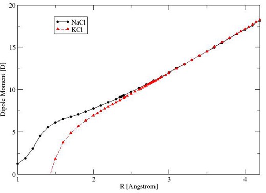
Ab initio DMCs for NaCl and KCl in their ground electronic states.
2.4 Fitting the potentials
The PECs were refined by fitting to the spectroscopic data identified in Table 1. However, extending the temperature range of the spectra requires consideration of highly excited levels and extrapolation of the PECs beyond the region determined by experimental input values; hence, care needs to be taken to ensure that the curves maintain physical shapes outside the experimentally refined regions. In this context, we define a physical shape to be the shape of the ab initio curve. We tested multiple potential energy forms, namely the extended Morse oscillator (EMO), Morse long range (MLR) and Morse–Lennard Jones potentials (Le Roy 2011), to achieve an optimum fit to the experimental data whilst maintaining a physical curve shape. Data for multiple isotopologues were fitted simultaneously to ensure that the resulting curves are valid for all isotopologues. re and De were held constant in the fits, as the fits were found to be unstable otherwise.
Computed values of the KCl dipole, μ, as a function of bond length, R.
| R (Å) | μ (D) | R (Å) | μ (D) | R (Å) | μ (D) | R (Å) | μ (D) |
|---|---|---|---|---|---|---|---|
| 1.5 | 1.830 345 58 | 2.4 | 8.996 620 28 | 2.76 | 10.772 468 | 3.3 | 13.490 959 15 |
| 1.6 | 3.739 305 15 | 2.42 | 9.095 698 99 | 2.77 | 10.821 950 94 | 3.4 | 14.005 846 02 |
| 1.7 | 4.869 647 22 | 2.45 | 9.244 043 43 | 2.78 | 10.871 458 14 | 3.5 | 14.524 113 63 |
| 1.8 | 5.674 082 82 | 2.5 | 9.490 746 12 | 2.79 | 10.920 990 47 | 3.6 | 15.045 513 41 |
| 1.9 | 6.334 728 37 | 2.55 | 9.737 0491 | 2.8 | 10.970 548 67 | 3.7 | 15.569 756 19 |
| 2 | 6.922 318 76 | 2.6 | 9.983 220 69 | 2.82 | 11.069 745 68 | 3.8 | 16.096 523 74 |
| 2.05 | 7.199 4271 | 2.62 | 10.081 704 13 | 2.85 | 11.218 753 05 | 3.9 | 16.625 479 73 |
| 2.1 | 7.468 781 85 | 2.65 | 10.229 485 29 | 2.88 | 11.368 029 41 | 3.95 | 16.890 670 47 |
| 2.15 | 7.732 1183 | 2.68 | 10.377 3678 | 2.9 | 11.467 703 66 | 4 | 17.156 2775 |
| 2.2 | 7.990 770 44 | 2.7 | 10.476 029 71 | 2.95 | 11.717 464 27 | 4.05 | 17.422 257 12 |
| 2.25 | 8.245 785 51 | 2.72 | 10.574 761 44 | 3 | 11.968 082 68 | 4.1 | 17.688 565 35 |
| 2.3 | 8.498 000 13 | 2.74 | 10.673 571 52 | 3.1 | 12.472 017 09 | 4.15 | 17.955 158 96 |
| 2.35 | 8.748 0928 | 2.75 | 10.723 008 51 | 3.2 | 12.979 644 97 | 4.2 | 18.221 994 22 |
Comparison of Na35Cl and 39K35Cl dipole moments at equilibrium internuclear distance.
Comparison of Na35Cl and 39K35Cl dipole moments at equilibrium internuclear distance.
Fitting parameters used in the NaCl EMO potential, see equation (1). (Uncertainties are given in parentheses in units of the last digit.)
| N | βi |
|---|---|
| 0 | 0.894 7078(17) |
| 1 | −0.287 528(48) |
| 2 | 0.005 81(11) |
| 3 | −0.0278(14) |
| 4 | −0.0290(37) |
| N | βi |
|---|---|
| 0 | 0.894 7078(17) |
| 1 | −0.287 528(48) |
| 2 | 0.005 81(11) |
| 3 | −0.0278(14) |
| 4 | −0.0290(37) |
Fitting parameters used in the KCl MLR potential, see equation (4). (Uncertainties are given in parentheses in units of the last digit.)
| N | βi | tj |
|---|---|---|
| 0 | −0.907 5210(10) | 0.0 |
| 1 | 1.235 90(85) | 0.00 30(12) |
| 2 | 0.4859(22) | 0.0 |
| 3 | 1.200(10) | 0.0 |
| N | βi | tj |
|---|---|---|
| 0 | −0.907 5210(10) | 0.0 |
| 1 | 1.235 90(85) | 0.00 30(12) |
| 2 | 0.4859(22) | 0.0 |
| 3 | 1.200(10) | 0.0 |
The input experimental data were reproduced within 0.01 cm−1 and often much better than this. The final curves, shown in Fig 2, follow the ab initio shape with the exception of regions 6–17 Å for KCl and 4.5–8 Å for NaCl. These regions are associated with the textbook avoided crossings between Columbic X+–Cl− and neutral X–Cl PECs which occur in the adiabatic representation of the ground electronic state, see Giese & York (2004) for a detailed discussion. Without experimental data near dissociation, it is difficult to represent this accurately with dpotfit. Consequently, we decided to limit our line lists to vibrational states lying below 20 000 cm−1 which do not sample these regions. This has consequences for the temperature range considered. Based on our partition sum, see Section 2.5, this range is 0–3000 K.
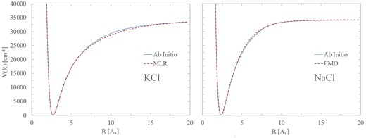
Comparison of ab initio and fitted ground electronic state PECs for NaCl (right) and KCl (left).
Comparisons with observed frequencies for Na35Cl and 39K35Cl are given in Tables 8 and 9. These demonstrate the accuracy of our fits. An important aim in refining a PEC is to also predict spectroscopic data outside the experimental range. This can be tested for KCl for which there are R-band head measurements up to v = 12 (Ram et al. 1997). The positions of these band heads, which are key features in any weak or low-resolution spectrum, are predicted to high accuracy, see Table 10.
Comparison of theoretically predicted Na35Cl ro-vibrational wavenumbers, in cm−1, with some of the laboratory measurements of Ram et al. (1997).
| v′ | J′ | v′′ | J′′ | Obs. | Calc. | Obs.−Calc. |
|---|---|---|---|---|---|---|
| 1 | 99 | 0 | 98 | 387.0444 | 387.0446 | −0.0002 |
| 1 | 100 | 0 | 99 | 387.1219 | 387.1221 | −0.0002 |
| 1 | 101 | 0 | 100 | 387.1950 | 387.1957 | −0.0007 |
| 2 | 3 | 1 | 2 | 358.9248 | 358.9260 | −0.0012 |
| 2 | 4 | 1 | 3 | 359.3419 | 359.3444 | −0.0025 |
| 2 | 5 | 1 | 4 | 359.7587 | 359.7596 | −0.0009 |
| 3 | 110 | 2 | 109 | 380.2722 | 380.2746 | −0.0024 |
| 3 | 111 | 2 | 110 | 380.3014 | 380.3075 | −0.0061 |
| 3 | 112 | 2 | 111 | 380.3372 | 380.3365 | 0.0007 |
| 4 | 28 | 3 | 27 | 361.3425 | 361.3429 | −0.0004 |
| 4 | 29 | 3 | 28 | 361.6718 | 361.6730 | −0.0012 |
| 4 | 31 | 3 | 30 | 362.3244 | 362.3230 | 0.0014 |
| 5 | 3 | 4 | 2 | 348.6060 | 348.6104 | −0.0044 |
| 5 | 4 | 4 | 3 | 349.0193 | 349.0195 | −0.0002 |
| 5 | 5 | 4 | 4 | 349.4289 | 349.4254 | 0.0035 |
| 6 | 114 | 5 | 113 | 369.5373 | 369.5406 | −0.0033 |
| 6 | 115 | 5 | 114 | 369.5551 | 369.5562 | −0.0011 |
| 6 | 117 | 5 | 116 | 369.5781 | 369.5758 | 0.0023 |
| 7 | 73 | 6 | 72 | 362.1649 | 362.1606 | 0.0043 |
| 7 | 74 | 6 | 73 | 362.3244 | 362.3276 | −0.0032 |
| 7 | 75 | 6 | 74 | 362.4924 | 362.4910 | 0.0014 |
| 8 | 38 | 7 | 37 | 350.7058 | 350.7009 | 0.0049 |
| 8 | 39 | 7 | 38 | 350.9881 | 350.9876 | 0.0005 |
| 8 | 40 | 7 | 39 | 351.2687 | 351.2710 | −0.0023 |
Comparison of theoretically predicted 39K35Cl ro-vibrational wavenumbers, in cm−1, with some of the laboratory data of Ram et al. (1997), as re-assigned in this work.
| v′ | J′ | v′′ | J′′ | Obs. | Calc. | Obs.−Calc. |
|---|---|---|---|---|---|---|
| 1 | 102 | 0 | 101 | 294.9349 | 294.9347 | 0.0002 |
| 1 | 103 | 0 | 102 | 295.0173 | 295.0154 | 0.0019 |
| 1 | 104 | 0 | 103 | 295.0955 | 295.0941 | 0.0014 |
| 1 | 105 | 0 | 104 | 295.1729 | 295.1710 | 0.0019 |
| 2 | 43 | 1 | 42 | 284.5787 | 284.5795 | −0.0008 |
| 2 | 49 | 1 | 48 | 285.6588 | 285.6551 | 0.0037 |
| 2 | 51 | 1 | 50 | 286.0004 | 286.0001 | 0.0003 |
| 2 | 52 | 1 | 51 | 286.1646 | 286.1700 | −0.0054 |
| 3 | 121 | 2 | 120 | 291.1544 | 291.1554 | −0.0010 |
| 3 | 122 | 2 | 121 | 291.2013 | 291.1992 | 0.0021 |
| 3 | 123 | 2 | 122 | 291.2433 | 291.2411 | 0.0022 |
| 3 | 126 | 2 | 125 | 291.3562 | 291.3555 | 0.0007 |
| 4 | 74 | 3 | 73 | 284.6069 | 284.6019 | 0.0050 |
| 4 | 75 | 3 | 74 | 284.7309 | 284.7300 | 0.0009 |
| 4 | 76 | 3 | 75 | 284.8579 | 284.8563 | 0.0016 |
| 4 | 78 | 3 | 77 | 285.1054 | 285.1036 | 0.0018 |
| 5 | 111 | 4 | 110 | 285.7192 | 285.7174 | 0.0018 |
| 5 | 113 | 4 | 112 | 285.8341 | 285.8375 | −0.0034 |
| 5 | 114 | 4 | 113 | 285.8912 | 285.8947 | −0.0035 |
| 5 | 116 | 4 | 115 | 286.0004 | 286.0037 | −0.0033 |
| 6 | 73 | 5 | 72 | 279.6821 | 279.6817 | 0.0004 |
| 6 | 75 | 5 | 74 | 279.9388 | 279.9355 | 0.0033 |
| 6 | 76 | 5 | 75 | 280.0552 | 280.0598 | −0.0047 |
| 6 | 81 | 5 | 80 | 280.6586 | 280.6552 | 0.0034 |
Comparison of theoretically predicted 39K35Cl R-branch band heads, in cm−1, with laboratory measurements from Ram et al. (1997) and this work.
| Band | Observed | Calculated | O − C |
|---|---|---|---|
| 1–0 | 296.702 | 296.703 | −0.001 |
| 2–1 | 294.181 | 294.182 | −0.001 |
| 3–2 | 291.680 | 291.682 | −0.002 |
| 4–3 | 289.201 | 289.203 | −0.002 |
| 5–4 | 286.742 | 286.745 | −0.003 |
| 6–5 | 284.303 | 284.306 | −0.003 |
| 7–6 | 281.884 | 281.887 | −0.003 |
| 8–7 | 279.488 | 279.489 | −0.001 |
| 9–8 | 277.110 | 277.110 | 0.0 |
| 10–9 | 274.752 | 274.752 | 0.0 |
| 11–10 | 272.414 | 272.411 | 0.003 |
| 12–11 | 270.120 | 270.090 | 0.03 |
2.5 Partition functions
The calculated energy levels, see Section 3, were summed in Excel to generate partition function values for a range of temperatures. We determined that our partition function is at least 95 per cent converged at 3000 K and much better than this at lower temperatures. Therefore, temperatures up to 3000 K were considered. Values for the parent isotopologues are compared to previous studies, namely Irwin (1981), Sauval & Tatum (1984) and CDMS, in Table 11.
Comparison of Na35Cl and 39K35Cl partition functions.
| T (K) | This work | CDMS | Irwin (1981) | Sauval & Tatum (1984) |
|---|---|---|---|---|
| Na35Cl | ||||
| 9.375 | 30.3338 | 30.3307 | – | – |
| 18.75 | 60.3352 | 60.3299 | – | – |
| 37.5 | 120.3556 | 120.3455 | – | – |
| 75 | 240.6984 | 240.6770 | – | – |
| 150 | 496.6455 | 496.5538 | – | – |
| 225 | 802.3712 | 802.1167 | – | – |
| 300 | 1173.0397 | 1172.5403 | – | – |
| 500 | 2506.9232 | 2505.0340 | – | – |
| 1000 | 8161.702 | – | 8204.6 | 8165.4 |
| 1500 | 17 333.48 | – | 17 409.8 | 16 960.3 |
| 2000 | 30 294.77 | – | 30 370.1 | 29 685.3 |
| 2500 | 47 362.31 | – | 47 324.9 | 46 807.2 |
| 3000 | 68 909.60 | – | 68 530.1 | 68 766.1 |
| 39K35Cl | ||||
| 9.375 | 51.1529 | 51.1495 | – | – |
| 18.75 | 101.9823 | 101.9724 | – | – |
| 37.5 | 203.6737 | 203.6504 | – | – |
| 75 | 409.1563 | 409.1053 | – | – |
| 150 | 876.2078 | 876.0902 | – | – |
| 225 | 1474.9611 | 1474.7618 | – | – |
| 300 | 2225.1732 | 2224.8905 | – | – |
| 500 | 5000.7420 | 5000.3352 | – | – |
| 1000 | 17 102.33 | – | 17 277.73 | 17 112.5 |
| 1500 | 37 064.68 | – | 37 327.7 | 36 147.1 |
| 2000 | 65 580.22 | – | 65 747.4 | 64 142.9 |
| 2500 | 103 489.55 | – | 103 058.6 | 102 212.0 |
| 3000 | 151 831.71 | – | 149 837.7 | 151 368.0 |
Fitting parameters used to fit the partition functions, see equation 10. Fits are valid for temperatures between 500 and 3000 K.
| Na35Cl | Na37Cl | 39K35Cl | 39K37Cl | 41K35Cl | 41K37Cl | |
|---|---|---|---|---|---|---|
| a0 | 35.528 812 | 39.941 335 | 71.922 595 | 72.206 029 | 74.926 932 | 72.591 531 |
| a1 | −65.142 353 | −73.363 68 | −138.068 267 | −138.340 7430 | −143.689 312 | −139.093 018 |
| a2 | 53.290 409 | 59.657 6584 | 114.111 9477 | 114.101 455 00 | 118.474 798 | 114.705 511 |
| a3 | −23.592 248 | −26.212 185 | −50.527 0109 | −50.414 764 00 | −52.319 838 | −50.665 015 |
| a4 | 6.036 705 | 6.641 337 62 | 12.738 250 | 12.683 942 00 | 13.150 0522 | 12.740 842 |
| a5 | −0.837 0958 | −0.911 3382 | −1.726 9110 | −1.716 340 70 | −1.777 0609 | −1.723 0912 |
| a6 | 0.048 872 72 | 0.052 663 06 | 0.098 186 748 | 0.097 426 548 | 0.100 716 4997 | 0.097 752 6634 |
2.6 Line-list calculations
While sodium has only a single stable isotope, 23Na, both potassium and chlorine each have two: 39K (whose natural terrestrial abundance is about 93.25 per cent) and 41K (6.73 per cent), and 35Cl (75.76 per cent) and 37Cl (24.24 per cent). Line lists were therefore calculated for two NaCl and four KCl isotopologues. Ro-vibrational states up to v = 100, J = 563 and v = 120, J = 500, respectively, and all transitions between these states satisfying the dipole selection rule ΔJ = ±1, were considered. A summary of each line list is given in Table 13.
Summary of our line lists.
| Na35Cl | Na37Cl | 39K35Cl | 39K37Cl | 41K35Cl | 41K37Cl | |
|---|---|---|---|---|---|---|
| Maximum v | 100 | 100 | 120 | 120 | 120 | 120 |
| Maximum J | 557 | 563 | 500 | 500 | 500 | 500 |
| Number of lines | 4734 567 | 4763 324 | 7224 331 | 7224 331 | 7224 331 | 7224 331 |
| Na35Cl | Na37Cl | 39K35Cl | 39K37Cl | 41K35Cl | 41K37Cl | |
|---|---|---|---|---|---|---|
| Maximum v | 100 | 100 | 120 | 120 | 120 | 120 |
| Maximum J | 557 | 563 | 500 | 500 | 500 | 500 |
| Number of lines | 4734 567 | 4763 324 | 7224 331 | 7224 331 | 7224 331 | 7224 331 |
The procedure described above was used to produce line lists, i.e. catalogues of transition frequencies νij and Einstein coefficients Aij for two NaCl and four KCl isotopologues: Na35Cl, Na37Cl, 39K35Cl, 39K37Cl, 41K35Cl and 41K37Cl. The computed line lists are available in electronic form as supplementary information to this paper.
3 RESULTS
The full line list computed for all isotopologue considered is summarized in Table 13. Each line list contains around 4 million transitions for NaCl and 7 million for the heavier KCl isotopologues; each line list is therefore, for compactness and ease of use, divided into a separate energy file and transition file. This is done using the standard ExoMol format (Tennyson, Hill & Yurchenko 2013) which is based on a method originally developed for the BT2 line list (Barber et al. 2006). Extracts from the start of the Na35Cl and 39K35Cl files are given in Tables 14 – 17. They can be downloaded from the CDS via http://cdsweb.u-strasbg.fr/cgi-bin/qcat?J/MNRAS/http://cdsweb.u-strasbg.fr/cgi-bin/qcat?J/MNRAS/. The line lists and partition functions can also be obtained from www.exomol.com.
Extract from start of states file for Na35Cl.
| I | |$\tilde{E}$| | g | J | v |
|---|---|---|---|---|
| 1 | 0.000 000 | 16 | 0 | 0 |
| 2 | 0.434 501 | 48 | 1 | 0 |
| 3 | 1.303 497 | 80 | 2 | 0 |
| 4 | 2.606 971 | 112 | 3 | 0 |
| 5 | 4.344 901 | 144 | 4 | 0 |
| 6 | 6.517 259 | 176 | 5 | 0 |
| I | |$\tilde{E}$| | g | J | v |
|---|---|---|---|---|
| 1 | 0.000 000 | 16 | 0 | 0 |
| 2 | 0.434 501 | 48 | 1 | 0 |
| 3 | 1.303 497 | 80 | 2 | 0 |
| 4 | 2.606 971 | 112 | 3 | 0 |
| 5 | 4.344 901 | 144 | 4 | 0 |
| 6 | 6.517 259 | 176 | 5 | 0 |
I: state counting number; |$\tilde{E}$|: state energy in cm−1; g: state degeneracy; J: state rotational quantum number; v: state vibrational quantum number.
Extract from start of states file for 39K35Cl.
| I | |$\tilde{E}$| | g | J | v |
|---|---|---|---|---|
| 1 | 0.0 | 16 | 0 | 0 |
| 2 | 0.256 466 | 48 | 1 | 0 |
| 3 | 0.769 393 | 80 | 2 | 0 |
| 4 | 1.538 778 | 112 | 3 | 0 |
| 5 | 2.564 613 | 144 | 4 | 0 |
| 6 | 3.846 887 | 176 | 5 | 0 |
| I | |$\tilde{E}$| | g | J | v |
|---|---|---|---|---|
| 1 | 0.0 | 16 | 0 | 0 |
| 2 | 0.256 466 | 48 | 1 | 0 |
| 3 | 0.769 393 | 80 | 2 | 0 |
| 4 | 1.538 778 | 112 | 3 | 0 |
| 5 | 2.564 613 | 144 | 4 | 0 |
| 6 | 3.846 887 | 176 | 5 | 0 |
I: state counting number; |$\tilde{E}$|: state energy in cm−1; g: state degeneracy; J: state rotational quantum number; v: state vibrational quantum number.
Extracts from the transitions file for Na35Cl.
| I | F | AIF |
|---|---|---|
| 2 | 1 | 7.21E−07 |
| 3 | 2 | 6.93E−06 |
| 4 | 3 | 2.50E−05 |
| 5 | 4 | 6.16E−05 |
| 6 | 5 | 1.23E−04 |
| 7 | 6 | 2.16E−04 |
| I | F | AIF |
|---|---|---|
| 2 | 1 | 7.21E−07 |
| 3 | 2 | 6.93E−06 |
| 4 | 3 | 2.50E−05 |
| 5 | 4 | 6.16E−05 |
| 6 | 5 | 1.23E−04 |
| 7 | 6 | 2.16E−04 |
I: upper state counting number; F: lower state counting number; AIF: Einstein A coefficient in s−1.
Extracts from the transitions file for 39K35Cl.
| I | F | AIF |
|---|---|---|
| 2 | 1 | 1.89E−07 |
| 3 | 2 | 1.81E−06 |
| 4 | 3 | 6.55E−06 |
| 5 | 4 | 1.61E−05 |
| 6 | 5 | 3.21E−05 |
| 7 | 6 | 5.64E−05 |
| I | F | AIF |
|---|---|---|
| 2 | 1 | 1.89E−07 |
| 3 | 2 | 1.81E−06 |
| 4 | 3 | 6.55E−06 |
| 5 | 4 | 1.61E−05 |
| 6 | 5 | 3.21E−05 |
| 7 | 6 | 5.64E−05 |
I: upper state counting number; F: lower state counting number; AIF: Einstein A coefficient in s−1.
Fig. 3 illustrates the synthetic absorption spectra of Na35Cl and 39K35Cl at 300 K. As the DMCs are essentially straight lines, the overtone bands for these molecules are very weak meaning that key spectral features are confined to long wavelengths associated with the pure rotational spectrum and the vibrational fundamental.
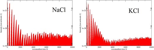
Absorption spectra of Na35Cl and 39K35Cl at 300 K.
The CDMS data base contains 607 and 772 rotational lines for Na35Cl and 39K35Cl, respectively. Comparisons with the CDMS lines are presented in Fig. 4. As can be seen, the agreement is excellent for both frequency and intensity. In particular, predicted line intensities agree within 2 and 4 per cent for the KCl and NaCl isotopomers considered in CDMS, respectively.
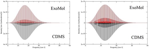
Absorption lines of Na35Cl and 39K35Cl at 300 K: ExoMol versus CDMS.
Emission cross-sections for Na35Cl and 39K35Cl were simulated using Gaussian line-shape profiles with half-width = 0.01 cm−1 as described by Hill, Yurchenko & Tennyson (2013). The resulting synthetic emission spectra are compared to the experimental ones in Figs 5 and 6. When making comparisons, one has to be aware of a number of experimental issues. The baseline in NaCl shows residual ‘channelling’: a sine-like baseline that often appears in FTS spectra due to interference from reflections from parallel optical surfaces in the beam. For KCl, the spectrum is very weak and the baseline, which has a large offset, was not properly adjusted to zero. Given these considerations, the comparisons must be regarded as satisfactory.
![Emission spectra of NaCl at 1273 K: left, Ram et al. (1997); right, ExoMol. [Reprinted from Ram et al. (1997). Copyright 1997, with permission from Elsevier.]](https://oup.silverchair-cdn.com/oup/backfile/Content_public/Journal/mnras/442/2/10.1093/mnras/stu944/2/m_stu944fig5.jpeg?Expires=1749903851&Signature=xOXGVcw~arjuA7~6eLTZiKLszT923udBjHU6u2OgbSNj25J7tVnvrUCmdc~H6d19S1avTd37An95EcWn3qsXqdcmz71D2fiGAPu0xmgjJM9plsS4gW-Stb1ZlkZIycO9jwnlXJOZOO0f9VwhmesKgAPZlGbPu0ilCPc9S0pYgDscWoKRk3ItyUp0oJ63JugE809Yefueh7tU4JUtN9D51Xh3ZPKcWyDrNicG82Q6AXqx7-H8YDsHfDJ1-Pwb3TUG5Ka6JO~xBe6DmtnXk~BYPJZPUvdF9X9fJu2qqVsoDd7Bc1loHsF6bl~2mEVmuj302TaFaFRhomadAOQstXok3w__&Key-Pair-Id=APKAIE5G5CRDK6RD3PGA)
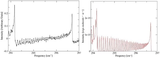
Emission spectra of KCl at 1273 K: left, Ram et al. (1997); right, ExoMol.
4 CONCLUSIONS
We present accurate but comprehensive line lists for the stable isotopologues of NaCl and KCl. Laboratory frequencies are reproduced to much more than sub-wavenumber accuracy. This accuracy should extend to all predicted transition frequencies up to at least v = 8 and 12 for NaCl and KCl, respectively. New ab initio dipole moments and Einstein A coefficients are computed. Comparisons with the semi-empirical CDMS data base suggest that the pure rotational intensities are accurate.
The results are line lists for the rotation–vibration transitions within the ground states of Na35Cl, Na37Cl, 39K35Cl, 39K37Cl, 41K35Cl and 41K37Cl, which should be accurate for a range of temperatures up to at least 3000 K. The line lists can be downloaded from the CDS or from www.exomol.com.
Finally, we note that HCl is likely to be the other main chlorine-bearing species in exoplanets. Comprehensive line lists for H35Cl and H37Cl have recently been provided by Li et al. (2013a,b).
We thank Alexander Fateev for stimulating discussions and Kevin Kindley for some preliminary work with the KCl infrared emission spectrum. This work was supported by grant from energinet.dk under a subcontract from the Danish Technical University and by the ERC under the Advanced Investigator Project 267219. Support was also provided by the NASA Origins of Solar Systems programme.
