


Abstract
We present an updated version of the so-called Madau model for attenuation of the radiation from distant objects by intergalactic neutral hydrogen. First, we derive the distribution function of intergalactic absorbers from the latest observational statistics of the Lyα forest, Lyman-limit systems and damped Lyα systems. The distribution function reproduces the observed redshift evolution of the Lyα depression and the mean-free path of the Lyman continuum excellently and simultaneously. We then derive a set of analytic functions describing the mean intergalactic attenuation curve for objects at z > 0.5. The new model predicts less (or more) Lyα attenuation for z ≃ 3–5 (z > 6) sources through the usual broad-band filters relative to the original Madau model. This may cause a systematic difference in the photometric redshift estimates, which is, however, still small: about 0.05. Finally, we find a more than 0.5 mag overestimation of Lyman-continuum attenuation in the original Madau model at z > 3, which causes a significant overcorrection against direct observations of the Lyman continuum of galaxies.
1 INTRODUCTION
Radiation from cosmological sources is absorbed by neutral hydrogen left in the intergalactic medium (IGM) even after cosmic reionization (e.g. Gunn & Peterson 1965). This intergalactic neutral hydrogen probably traces the ‘cosmic web’ produced by the gravity of dark matter (e.g. Rauch 1998). Along an observer's line of sight piercing the cosmic web, there appear to be numerous discrete systems composed of intergalactic neutral hydrogen, producing a number of absorption lines in the spectra of distant sources. These systems are divided into the Lyα forest (LAF: |$\log _{10}(N_{\rm H\,\small {I}}/{\rm cm}^{-2})<17.2$|), Lyman-limit systems (LLSs: |$17.2\le \log _{10}(N_{\rm H\,\small {I}}/{\rm cm}^{-2})<20.3$|) and damped Lyα systems (DLAs: |$\log _{10}(N_{\rm H\,\small {I}}/{\rm cm}^{-2})\ge 20.3$|), depending on the column density of the neutral hydrogen along the line of sight (e.g. Rauch 1998).
Intergalactic absorption is routinely found in the spectra of objects at a cosmological distance and this feature is utilized as a tool to select high-z objects only by photometric data: the so-called drop-out technique (e.g. Steidel, Pettini & Hamilton 1995; Madau et al. 1996). To put it another way, we must always correct the spectra of cosmological sources for this absorption in order to know the intrinsic properties. Therefore, an accurate model of this absorption is quite useful as a standard tool for observational cosmology.
After several models for this purpose were presented (e.g. Møller & Jakobsen 1990; Zuo 1993; Yoshii & Peterson 1994), that of Madau (1995, hereafter M95) appeared and became the most popular because of its convenient analytic functions. However, the heart of the model, i.e. the statistics of the LAF, LLSs and DLAs, has been updated greatly by observations in the last two decades since M95. In fact, there are several articles adopting such updated statistics (Bershady, Charlton & Geoffroy 1999; Meiksin 2006; Tepper-García & Fritze 2008; Inoue & Iwata 2008). Nevertheless, people still adhere to M95, except for a few innovative authors (e.g. Harrison, Meiksin & Stock 2011; Overzier et al. 2013). This adherence may be due to the simplicity and convenience of the analytic functions in M95. Here, in this article, we intend to present a user-friendly analytic function conforming to the updated statistics.
In the next section, we introduce the heart of the modelling: the distribution function of intergalactic absorbers derived from the latest observational data of the LAF, LLSs and DLAs. We then show the updated mean transmission function and compare it with the latest observations of Lyα transmission and the mean-free path of Lyman-limit photons in Section 3. In Section 4, we present new analytic formulae for intergalactic attenuation. Finally, we quantify the difference in attenuation magnitudes between the M95 model and ours through some broad-band filters and discuss the effect on the drop-out technique and photometric redshift estimation in Section 5. We do not need to assume any specific cosmological model in this article, except in Sections 2.1 and 3.2, where we assume ΩM = 0.3, ΩΛ = 0.7 and H0 = 70 km s−1 Mpc−1. Therefore, the analytic functions presented in Section 4 can be used directly in any cosmological model.
2 DISTRIBUTION FUNCTION OF INTERGALACTIC ABSORBERS

Number of intergalactic absorbers per unit column density of neutral hydrogen (|$N_{\rm H\,\small {I}}$|) per unit absorption length (X) along an average line of sight as a function of the column density. (a) The redshift evolution of the functions in Madau (1995). (b) The same as (a), but for the model in Inoue & Iwata (2008). (c) The same as (a), but for the model of this work. (d) A comparison of the three models with the observational data at z ∼ 2.5 taken from the literature: Kim et al. (2013) for LAF, O'Meara et al. (2013) for LLSs, Prochaska et al. (2014) for sub-DLAs (original data presented by O'Meara et al. 2007) and Noterdaeme et al. (2013) for DLAs. The solid, dotted and dashed lines denote the models of this work, Inoue & Iwata (2008) and Madau (1995), respectively. The two thin solid lines show the LAF and DLA components in this work.
Parameters for the distribution function of intergalactic absorbers assumed in this article.
| Common | |||||||
| Parameter | log10(Nl/cm−2) | log10(Nu/cm−2) | log10(Nc/cm−2) | 〈b/kms−1〉 | |||
| Value | 12 | 23 | 21 | 28 | |||
| LAF component | |||||||
| Parameter | |${\cal A}_{\rm LAF}$| | βLAF | zLAF, 1 | zLAF, 2 | γLAF, 1 | γLAF, 2 | γLAF, 3 |
| Value | 500 | 1.7 | 1.2 | 4.7 | 0.2 | 2.7 | 4.5 |
| DLA component | |||||||
| Parameter | |${\cal A}_{\rm DLA}$| | βDLA | zDLA, 1 | — | γDLA, 1 | γDLA, 2 | — |
| Value | 1.1 | 0.9 | 2.0 | — | 1.0 | 2.0 | — |
2.1 Column density distribution
M95 adopted a single power-law index of −1.5 (e.g. Tytler 1987). However, recent observations suggest a break of the column density distribution around |$N_{\rm H\,\small {I}}\sim 10^{17}$| cm−2 (Prochaska, Herbert-Fort & Wolfe 2005; Prochaska, O'Meara & Worseck 2010; O'Meara et al. 2013); the slope changes from a steeper one at lower column densities to a shallower one at higher column densities. The break column density is about the threshold of LLSs; the optical depth against Lyman-limit photons is about unity with this column density. Therefore, this break is probably caused by the transition between optically thin and thick against the ionizing background radiation (Corbelli, Salpeter & Bandiera 2001; Corbelli & Bandiera 2002). Indeed, the latest cosmological radiation hydrodynamics simulations show that self-shielding of optically thick absorbers is the mechanism producing the break (Altay et al. 2011; Rahmati et al. 2013). On the other hand, M95 has a discontinuity in the column density, as found in Fig. 1(a), owing to the different redshift evolution of the LAF and LLSs.
II08 adopted a double power-law function in order to describe the break at |$N_{\rm H\,\small {I}}\sim 10^{17}$| cm−2. In fact, they assumed a break column density |$N_{\rm H\,\small {I}}=1.6\times 10^{17}$| cm−2 at which the optical depth against Lyman-limit photons becomes unity. With this double power-law function for the column density distribution, II08 assumed a universal redshift evolution for all column densities. As a result, the number densities of LLSs and DLAs per unit absorption length increase monotonically with redshift, as found in Fig. 1(b). However, recent observations suggest a much weaker evolution of DLAs (Prochaska et al. 2005; O'Meara et al. 2013) and the cosmological simulations reproduce this weak evolution successfully (Rahmati et al. 2013).
In this article, we have assumed in equation (5) a power-law function with an exponential cut-off like the Schechter function. Such a functional shape has already been proposed by Prochaska et al. (2005) to describe the column density distribution of DLAs. As found at the highest column densities in Fig. 1(d), this function reproduces the DLA distribution very well if we adopt a cut-off column density Nc ≃ 1021 cm−2. With this functional shape, we successfully reproduce the weak evolution of the column density distribution of DLAs as shown in Fig. 1(c). This is partly due to a weaker redshift evolution in the DLA regime of this article than in II08, as discussed in Fig. 2 below, but the constancy of the cut-off column density is also important. On the other hand, M95 also predicts almost no evolution of LLSs due to weak redshift evolution for absorbers of high column density (see equation 2). However, the M95 model does not have any DLAs.
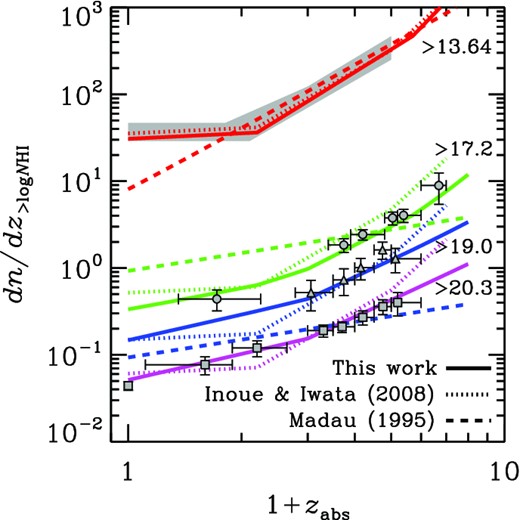
Number of intergalactic absorbers per unit redshift along an average line of sight as a function of absorber redshift. The shaded area is the observed range for absorbers with |$\log _{10}(N_{\rm H\,\small {I}}/{\rm cm}^{-2})>13.6$| (LAF) taken from Weymann et al. (1998), Kim, Cristiani & D'Odorico (2001) and Janknecht et al. (2006). The filled circles, triangles and squares are observed data of absorbers with |$\log _{10}(N_{\rm H\,\small {I}}/{\rm cm}^{-2})>17.2$| (LLS) taken from Songaila & Cowie (2010), >19.0 (sub-DLA) taken from Péroux et al. (2005) and >20.3 (DLA) taken from Rao, Turnshek & Nestor (2006), respectively. The solid, dotted and dashed lines denote the models of this work, Inoue & Iwata (2008) and Madau (1995). Note that the Madau (1995) model does not have DLAs.
2.2 Number density evolution
Next, we look into the number density evolution with redshift. Fig. 2 shows a comparison of the models with observations for four categories of absorbers depending on the column density: |$\log _{10}(N_{\rm H\,\small {I}}/{\rm cm}^{-2})>13.64$| (LAF), >17.2 (LLSs), >19.0 (sub-DLAs or super-LLSs) and >20.3 (DLAs). Fig. 3 shows a close-up of LLS evolution.
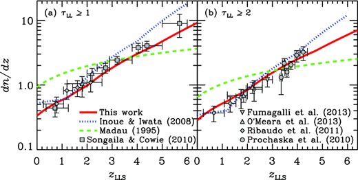
Number of LLSs per unit redshift along an average line of sight as a function of LLS redshift: (a) systems with optical depth for hydrogen Lyman-limit photons equal to or larger than unity and (b) systems with optical depth equal to or larger than two. The squares, diamonds, triangles, upside-down triangles and circles are the observed data taken from Songaila & Cowie (2010), Ribaudo, Lehner & Howk (2011), O'Meara et al. (2013), Fumagalli et al. (2013) and Prochaska et al. (2010), respectively. The solid, dotted and dashed lines denote the models of this work, Inoue & Iwata (2008) and Madau (1995), respectively.
M95 adopted a single power law of (1 + z). This fits well with the LAF number density evolution at z > 1, but it predicts too small a number density relative to observations at z < 1, where the observed number density is almost constant (Weymann et al. 1998). The break in the observed LAF number density evolution at z ∼ 1 is probably caused by the sharp decline of the ionizing background radiation from this epoch to the present (e.g. Davé et al. 1999). The LLS number evolution of M95 is largely different from that of observations in respect of the slope, while the absolute value matches the observations at z ∼ 3. Furthermore, the M95 model has too small a number of sub-DLAs and does not have any DLAs.
II08 adopted a twice-broken power law for the redshift evolution. The first break is set at z ∼ 1 to describe the bent of the LAF number evolution and the second break is set at z ∼ 4 to reproduce the rapid increase in Lyα optical depth towards high z (see the next section). The same function was assumed for all absorber categories in II08. It is still compatible with the observed LLS and sub-DLA evolution, but the agreement becomes marginal for DLAs.
In this article, we adopt two different forms of evolution for the LAF and DLA components. As found in Fig. 2, this new description shows the best agreement with observations for all absorber categories. Fig. 3 shows that the new model matches observations better than the II08 model. In particular, the new model tends to have a smaller number of LLSs than II08. This point is essential to reproduce the observed mean-free path for ionizing photons, as discussed in Section 3.2.
3 MEAN TRANSMISSION FUNCTION
With the distribution function of intergalactic absorbers described in the previous section, we can integrate equation (1) numerically and obtain the mean transmission function of the IGM. In the integration, we treat the neutral hydrogen cross-section |$\sigma ^{\rm H\,\small {I}}_{\lambda _{\rm abs}}$| as follows: we adopt the interpolation formula given by Osterbrock (1989) for the photoionization cross-section. We also adopt the oscillator strengths and the damping constants taken from Wiese, Smith & Glennon (1966) and the analytic formula of the Voigt profile given by Tepper-García (2006) for the Lyman series cross-sections. The mean Doppler velocity is assumed to be 〈b〉 = 28 km s−1, obtained from the b distribution function proposed by Hui & Rutledge (1999), and its parameter bσ = 23 km s−1, as measured by Janknecht et al. (2006) for this work (see Table 1) and II08. On the other hand, we adopt 〈b〉 = 35 km s−1 for M95, according to the original assumption. In the integration of equation (1), we should set the redshift step, Δz, to be fine enough to resolve the narrow width of the Lyman-series lines. We adopt Δz = 5 × 10⁻⁵ and have confirmed the convergence of the calculations.
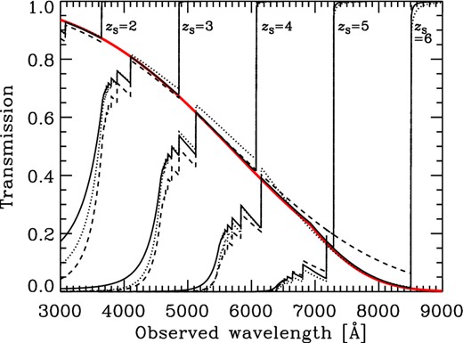
Fig. 4 shows the mean transmission functions obtained. The three models are very similar, but some differences are recognized if we look at them in detail. In the regime of Lyman-series transmission for zS ≤ 4, the II08 model is the highest, the M95 model is the lowest and the new model of this article is in the middle. On the other hand, the M95 model predicts the highest transmission for zS ≥ 5. However, the difference is small except for the case of zS = 6. This small difference comes from the small difference in the number density of the LAF, which is mainly responsible for Lyman-series absorption, among the three models, as seen in Fig. 2. The deviation of the M95 model found at wavelengths between Lyα and Lyβ for zS = 6 is due to the lack of rapid increase of the LAF number density at high z adopted in the other two models. This point will be discussed again in Fig. 5 below.
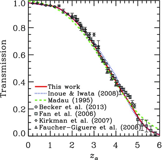
Lyα transmission as a function of the redshift of the Lyα line. The triangles, diamonds, squares and circles are observed data taken from Faucher-Giguère et al. (2008), Kirkman et al. (2007), Fan et al. (2006) and Becker et al. (2013), respectively. The solid, dotted and dashed lines are the models of this work, Inoue & Iwata (2008) and Madau (1995), respectively.
In the Lyman-continuum regime, the new model predicts the highest transmission, while the M95 model is the lowest for zS ≤ 4 and the II08 model is the lowest for zS ≥ 5 (but this is difficult to see in Fig. 4). Given that LLSs are mainly responsible for Lyman-continuum absorption, this difference is caused by the difference in number density of LLSs. Indeed, M95 has the largest density of LLSs at zLLS < 3 and the LLS density of II08 becomes the largest at zLLS > 3 (see Fig. 3). In the next two subsections, we compare model transmissions with observations in more detail in terms of Lyα transmission and the mean-free path for ionizing photons.
3.1 Lyα transmission
The spectrum between Lyα and Lyβ lines in the source rest frame is absorbed by the Lyα transition of neutral hydrogen in the IGM. This is called the Lyα depression (DA). Here we compare the three models discussed in this article with measurements of 1 −DA, i.e. Lyα transmission (Tα), in Fig. 5. M95 presented an analytic formula for the mean optical depth, which corresponds to the transmission as Tα = exp [−3.6 × 10⁻³(1 + zα)3.46], where zα = λobs/λα − 1 is the redshift of absorbers and the Lyα wavelength λα = 1215.67 Å. This formula is shown by the dashed line in Fig. 5. We have confirmed this formula from the mean transmission function, which we obtained from the integration of equation (1) with the M95 distribution function (equation 2).2 We derive analytic formulae for Tα from the mean transmission functions of the II08 model and our new model; these are shown by the dotted and solid lines in Fig. 5, respectively. The derivation is given in Section 4 below. We find that all three models agree excellently with observations. Among them, the new model presented in this article seems the best. In fact, the parameters for the LAF number density evolution with redshift of the new model (equation 6) were chosen so as to match the observed Tα. However, the agreement is not perfect at z ≃ 4.6, where the observed data deviate upwards from the model. Although we found better agreement with the data if we adopted a triple-break model instead of the double-break as in equation (6), we avoid it here to keep the model as simple as possible. If further observations emphasize the deviation, we should update the model again in future. On the other hand, the M95 model predicts slightly smaller Tα at 1 < z < 4 and larger Tα at other redshifts compared with the observed data. In particular, the M95 model deviates from observations at z > 5 because it does not have a rapid increase in LAF number density towards the epoch of reionization found in the last decade (e.g. Fan et al. 2006).
3.2 Mean-free path of ionizing photons
Fig. 6 shows the resultant mean-free paths. In Fig. 6(a), we show a comparison of the mean-free path taken from Worseck et al. (2014) with the three models discussed in this article. Their measurements are obtained through fits in the wavelength ranges 837–905 Å for z ∼ 4 (Prochaska et al. 2009), 700–911 Å for z = 2.4 (O'Meara et al. 2013), 830–905 Å for z = 3 (Fumagalli et al. 2013) and 850–910 Å for z > 4.5 (Worseck et al. 2014). These wavelength ranges are in the source rest-frame. We have made fittings of the mean transmission curves in the z = 2.4 and z ∼ 4 wavelength ranges and obtained the mean-free paths shown by the solid, dotted and dashed lines in Fig. 6(a). We find an excellent agreement between the new model and the observations. On the other hand, the II08 and M95 models predict shorter mean-free paths than the observations. At this stage, these old models have been inconsistent with the observations.
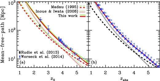
Mean-free path for hydrogen Lyman-limit photons as a function of (a) the source redshift and (b) the absorber redshift. (a) The circles with error bars are data taken from a compilation of Worseck et al. (2014). The solid, dotted and dashed lines are the estimates obtained from the mean transmission functions of this article, Inoue & Iwata (2008) and Madau (1995), respectively, using the PWO method (equations 11 and 12). The thick lines are estimates within the wavelength range 837–905 Å in the source rest-frame, which should be compared with the data at z ≥ 3. The thin lines are for range 700–911 Å, which should be compared with the data at z ∼ 2.4. (b) The solid, dotted and dashed lines are the same as in panel (a), but based on equations (13) and (14). The small squares are the same result as the solid thick line in panel (a); these are shifted to asterisks by conversion from the source redshift to the absorber redshift.
There is another recent measurement of the mean-free path at z ≈ 2.4 by Rudie et al. (2013), which is a factor of 2 shorter than that by O'Meara et al. (2013). According to Prochaska et al. (2014), the effects of line-blending and clustering of strong absorption systems like LLSs may cause such a discrepancy. In this article, we adopt the measurement by O'Meara et al. (2013) for z ≈ 2.4 and just show the measurement by Rudie et al. (2013) in Fig. 6(a) for comparison.
Fig. 6(b) shows the difference between the two definitions of the mean-free path introduced above (equations 12 and 14). The solid line is the mean-free path calculated from equation (14), but the small squares are calculated from equation (12): the PWO method. We find a small displacement between the two. We consider its origin to be the difference in redshifts; the displacement is horizontal, not vertical. The PWO method (equation 12) measures the mean-free path of photons with wavelength ≈870 Å at zS. However, the wavelength of these photons is redshifted to the Lyman limit at zabs, at which point equation (14) gives the mean-free path. If we convert zS in the PWO method into zabs, we obtain the asterisks and find excellent agreement of the two mean-free paths. Therefore, one should take care with the definition of the mean-free path in order to compare one result with another.
4 NEW ANALYTIC MODEL
4.1 Lyman-series absorption
For the Lyman-series absorption, let us approximate these cross-sections in the integral of equation (1) by a narrow rectangular shape function. For example, the Lyα cross-section is assumed to be σα(λ) = σα, 0 for λα − Δλ/2 < λ < λα + Δλ/2 and 0 otherwise, where σα, 0 is the cross-section at the line centre of the Lyα wavelength λα. The width Δλ can be expressed as (δb/c)λα, where δ is a numerical factor, b is the Doppler velocity and c is the light speed in vacuum. If we assume a Gaussian line profile and the cross-section integrated over the wavelength from 0 to ∞ to be equal to σα, 0Δλ, we obtain |$\delta =\sqrt{\pi }$|. However, the DLA component may contribute to the optical depth, especially for higher order Lyman-series lines, and in this case there may be a contribution from the damping wing to the cross-section, so that a larger δ value may be favourable. We thus determine the values of δ from comparison with the numerical integration later.
Wavelengths and coefficients for Lyman-series absorption.
| j | λj (Å) | |$A_{j,1}^{\rm LAF}$| | |$A_{j,2}^{\rm LAF}$| | |$A_{j,3}^{\rm LAF}$| | |$A_{j,1}^{\rm DLA}$| | |$A_{j,2}^{\rm DLA}$| |
|---|---|---|---|---|---|---|
| 2 (Lyα) | 1215.67 | 1.690e-02 | 2.354e-03 | 1.026e-04 | 1.617e-04 | 5.390e-05 |
| 3 (Lyβ) | 1025.72 | 4.692e-03 | 6.536e-04 | 2.849e-05 | 1.545e-04 | 5.151e-05 |
| 4 (Lyγ) | 972.537 | 2.239e-03 | 3.119e-04 | 1.360e-05 | 1.498e-04 | 4.992e-05 |
| 5 | 949.743 | 1.319e-03 | 1.837e-04 | 8.010e-06 | 1.460e-04 | 4.868e-05 |
| 6 | 937.803 | 8.707e-04 | 1.213e-04 | 5.287e-06 | 1.429e-04 | 4.763e-05 |
| 7 | 930.748 | 6.178e-04 | 8.606e-05 | 3.752e-06 | 1.402e-04 | 4.672e-05 |
| 8 | 926.226 | 4.609e-04 | 6.421e-05 | 2.799e-06 | 1.377e-04 | 4.590e-05 |
| 9 | 923.150 | 3.569e-04 | 4.971e-05 | 2.167e-06 | 1.355e-04 | 4.516e-05 |
| 10 | 920.963 | 2.843e-04 | 3.960e-05 | 1.726e-06 | 1.335e-04 | 4.448e-05 |
| 11 | 919.352 | 2.318e-04 | 3.229e-05 | 1.407e-06 | 1.316e-04 | 4.385e-05 |
| 12 | 918.129 | 1.923e-04 | 2.679e-05 | 1.168e-06 | 1.298e-04 | 4.326e-05 |
| 13 | 917.181 | 1.622e-04 | 2.259e-05 | 9.847e-07 | 1.281e-04 | 4.271e-05 |
| 14 | 916.429 | 1.385e-04 | 1.929e-05 | 8.410e-07 | 1.265e-04 | 4.218e-05 |
| 15 | 915.824 | 1.196e-04 | 1.666e-05 | 7.263e-07 | 1.250e-04 | 4.168e-05 |
| 16 | 915.329 | 1.043e-04 | 1.453e-05 | 6.334e-07 | 1.236e-04 | 4.120e-05 |
| 17 | 914.919 | 9.174e-05 | 1.278e-05 | 5.571e-07 | 1.222e-04 | 4.075e-05 |
| 18 | 914.576 | 8.128e-05 | 1.132e-05 | 4.936e-07 | 1.209e-04 | 4.031e-05 |
| 19 | 914.286 | 7.251e-05 | 1.010e-05 | 4.403e-07 | 1.197e-04 | 3.989e-05 |
| 20 | 914.039 | 6.505e-05 | 9.062e-06 | 3.950e-07 | 1.185e-04 | 3.949e-05 |
| 21 | 913.826 | 5.868e-05 | 8.174e-06 | 3.563e-07 | 1.173e-04 | 3.910e-05 |
| 22 | 913.641 | 5.319e-05 | 7.409e-06 | 3.230e-07 | 1.162e-04 | 3.872e-05 |
| 23 | 913.480 | 4.843e-05 | 6.746e-06 | 2.941e-07 | 1.151e-04 | 3.836e-05 |
| 24 | 913.339 | 4.427e-05 | 6.167e-06 | 2.689e-07 | 1.140e-04 | 3.800e-05 |
| 25 | 913.215 | 4.063e-05 | 5.660e-06 | 2.467e-07 | 1.130e-04 | 3.766e-05 |
| 26 | 913.104 | 3.738e-05 | 5.207e-06 | 2.270e-07 | 1.120e-04 | 3.732e-05 |
| 27 | 913.006 | 3.454e-05 | 4.811e-06 | 2.097e-07 | 1.110e-04 | 3.700e-05 |
| 28 | 912.918 | 3.199e-05 | 4.456e-06 | 1.943e-07 | 1.101e-04 | 3.668e-05 |
| 29 | 912.839 | 2.971e-05 | 4.139e-06 | 1.804e-07 | 1.091e-04 | 3.637e-05 |
| 30 | 912.768 | 2.766e-05 | 3.853e-06 | 1.680e-07 | 1.082e-04 | 3.607e-05 |
| 31 | 912.703 | 2.582e-05 | 3.596e-06 | 1.568e-07 | 1.073e-04 | 3.578e-05 |
| 32 | 912.645 | 2.415e-05 | 3.364e-06 | 1.466e-07 | 1.065e-04 | 3.549e-05 |
| 33 | 912.592 | 2.263e-05 | 3.153e-06 | 1.375e-07 | 1.056e-04 | 3.521e-05 |
| 34 | 912.543 | 2.126e-05 | 2.961e-06 | 1.291e-07 | 1.048e-04 | 3.493e-05 |
| 35 | 912.499 | 2.000e-05 | 2.785e-06 | 1.214e-07 | 1.040e-04 | 3.466e-05 |
| 36 | 912.458 | 1.885e-05 | 2.625e-06 | 1.145e-07 | 1.032e-04 | 3.440e-05 |
| 37 | 912.420 | 1.779e-05 | 2.479e-06 | 1.080e-07 | 1.024e-04 | 3.414e-05 |
| 38 | 912.385 | 1.682e-05 | 2.343e-06 | 1.022e-07 | 1.017e-04 | 3.389e-05 |
| 39 | 912.353 | 1.593e-05 | 2.219e-06 | 9.673e-08 | 1.009e-04 | 3.364e-05 |
| 40 | 912.324 | 1.510e-05 | 2.103e-06 | 9.169e-08 | 1.002e-04 | 3.339e-05 |
4.2 Lyman-continuum absorption
4.3 Validity of the analytic formulae
Let us confirm the validity of the approximate analytic formulae derived in the two subsections above. We compare the formulae with the numerical integration of equation (1). As a result, the contour in Fig. 7 shows the difference of the two optical depths divided by the numerical in the plane of the source redshift and the source rest-frame wavelength. We find that the differences are less than a few per cent over a large area when the source redshift is larger than 0.5. In the case of zS < 0.5, the observed wavelength for some rest-frame wavelengths on the horizontal axis becomes shorter than the Lyman limit and then the formulae for Lyman-continuum absorption in Section 4.2 become incorrect. As a result, the difference becomes >10 per cent. For zS > 0.5, the difference tends to be relatively large for higher order Lyman-series lines that the DLA component contributes to. Probably the rectangular shape approximation in the cross-section is not very good here. Nevertheless, the difference is still less than several per cent, 8 per cent at the most, ensuring the validity of the approximate formulae.
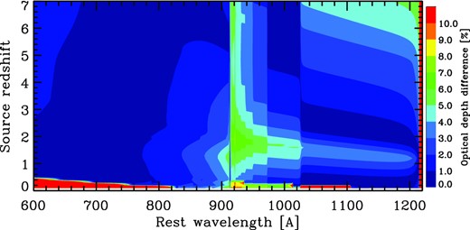
Fractional difference of the optical depths of the numerical integration of equation (1) and the approximate analytic formulae presented in Sections 4.1 and 4.2. The formulae break down at observed wavelengths shorter than the Lyman limit. As a result, there appear to be areas where the difference exceeds 10 per cent when the source redshift zS < 0.52.
5 DISCUSSION
Here we compare the attenuation magnitudes through some broad-band filters for the three models discussed in this article, quantify the difference and discuss the effect on the drop-out technique and the photometric redshift (hereafter photo-z) estimation.
Fig. 8 shows the IGM attenuation magnitudes through six broad-band filters as a function of source redshift in the case of βUV = −2.0, a flat continuum in Fν units usually observed in high-z star-forming galaxies (e.g. Shapley et al. 2003). We note here that the variation of βUV from −3 to 0 (e.g. Bouwens et al. 2009) has a negligible effect on the attenuation magnitudes. The solid, dotted and dashed lines are the models of this work, II08 and M95, respectively. The attenuation magnitudes shown in the figure are determined mainly by Lyα and Lyβ absorption. The difference seems to be small, as expected from the small difference in the mean transmission curves among the three models shown in Fig. 4. In fact, however, the vertical difference at a fixed source redshift reaches more than 1 mag between this work and the M95 model, while the horizontal difference is as small as about <0.2, except for the deviation of the M95 model at zS > 5.5, owing to the lack of rapid evolution of Lyα optical depth included in the other two models. The thin (coloured) solid lines are the results from the analytic formulae for the new model presented in the previous section. We find excellent agreement with the numerical integrations.
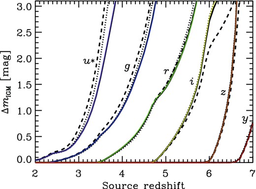
IGM attenuation magnitude through broad-band filters, the Canada–France–Hawaii Telescope/Mega-cam u* and the Subaru/Hyper Suprime-Cam g, r, i, z and y, as a function of source redshift. The solid, dotted and dashed lines are the models of this work, Inoue & Iwata (2008) and Madau (1995), respectively. The thin (coloured) solid lines are the cases using the analytic formulae for this work. An object spectrum with ultraviolet spectral index βUV = −2.0 is assumed.
Although the horizontal difference at a certain attenuation magnitude among the three models is small, there is a difference that would affect the drop-out technique and the photo-z estimation. The drop-out threshold is usually ΔmIGM ≃ 1 mag. The source redshift reaching the threshold is different from that of the models. For example, the redshifts in the M95 model are about 0.2 smaller than those of this work at zS ≃ 3–4 but about 0.1 larger at zS ≃ 6. These differences would result in systematically lower or higher photo-z solutions with the M95 model than with the new model of this article. To check this expectation, we ran the photo-z code developed by Tanaka et al. (2013a, b), adopting the two IGM models of this article and M95. The sample is galaxies with spectroscopic redshifts and photometry from the following instruments and bands: Very Large Telescope VIsible MultiObject Spectrograph (VLT/VIMOS) U, Hubble Space Telescope Advanced Camera for Surveys (HST/ACS) F435W, F606W, F775W, F814W, F850LP, Hubble Space Telescope Wide Field Camera 3 (HST/WFC3) F105W, F125W, F160W, Very Large Telescope Infrared Spectrometer And Array Camera (VLT/ISAAC) Ks and Spitzer InfraRed Array Camera (IRAC) Ch1 and Ch2 in the Great Observatories Origins Deep Survey South (GOODS-S) field (Guo et al. 2013). We collected spectroscopic redshifts from the literature (Le Fèvre et al. 2005; Mignoli et al. 2005; Vanzella et al. 2008; Popesso et al. 2009; Balestra et al. 2010) and cross-matched them with the photometric objects within 1 arcsec. We use secure redshifts only in the analysis here. The photo-z code assumes the stellar population synthesis model of Bruzual & Charlot (2003) with solar and subsolar metallicity models (Z = 0.02, 0.008 and 0.004), Chabrier initial mass function between 0.1 and 100 M⊙ (Chabrier 2003), exponentially declining star formation history, Calzetti attenuation law (Calzetti et al. 2000) and the emission-line model of Inoue (2011) with Lyman-continuum escape fraction of zero. The Lyα emission line is reduced by a factor of 0.1 to account for attenuation through the interstellar medium of galaxies. The metallicity, age, exponential time-scale of the history, dust attenuation amount and redshift are free parameters determined by a χ2 minimization technique. We compare the photo-z for the two IGM models in Fig. 9. We divided the sample galaxies into bins of 20 objects each and calculated the difference in means of the photo-z in each bin. The vertical error bars are estimated by |$\sqrt{\sum _i(\sigma _{\langle z_{{\rm ph},i}\rangle }^2/n+\delta _{z_{{\rm ph},i}}^2/n)}$|, where i indicates the two IGM models (this work and M95), |$\sigma _{\langle z_{{\rm ph},i}\rangle }$| is the standard deviation of the photo-z in each bin, |$\delta _{z_{{\rm ph},i}}$| is the mean of photo-z uncertainties of the sample galaxies in each bin and n = 20 is the number of sample galaxies in each bin. The first term is the standard error of the mean and the second term is the error in the mean propagated from the uncertainty in the individual photo-z. As found in Fig. 9, the difference in the means of photo-z is too small to be detected in the sample adopted, while we may find the expected trend of photo-z for the new IGM model to be larger (or smaller) than for the M95 model at z ≃ 3–5 (z > 5.5). The marginal difference of ≈0.05 at z ≃ 3.5 is much smaller than expected from Fig. 8. This is probably because we used not only the drop-out band but also all bands available in the photo-z estimation. As a result, the drop-out feature has lower weight in the photo-z determination. However, all available bands should be used in order to constrain the intrinsic shape of the spectral energy distribution below Lyα to characterize the IGM effect on photo-z. We would detect the IGM model difference securely if we had a ten times larger number of sample galaxies at z > 3.
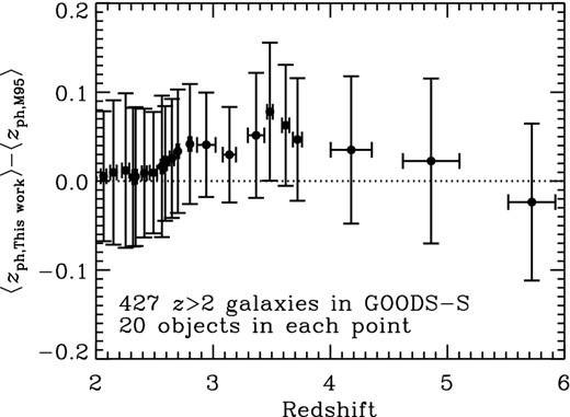
Difference in means of the photometric redshift estimations assuming the IGM model of this work relative to those assuming the Madau (1995) model. The sample is 427 galaxies with spectroscopic redshift larger than 2 in the GOODS-S field and is divided into bins of 20 objects each. Along the horizontal axis, the points and error bars show the mean and standard deviation of the spectroscopic redshifts in each bin. See the text for the vertical error bars.
Finally, we examine the mean IGM attenuation magnitude at a Lyman-continuum wavelength of 880 Å in the source rest-frame as a function of source redshift in Fig. 10. This is motivated by studies to determine an important parameter controlling the cosmic reionization, the Lyman-continuum escape fraction of galaxies (e.g. Inoue et al. 2005; Iwata et al. 2009; Inoue et al. 2011). In these studies, we need to correct the IGM attenuation against the observed Lyman continuum of galaxies. As found in Fig. 10, the difference among the three models discussed in this article is significant: the new model predicts the lowest attenuation, which is 0.5–1 mag smaller than for the M95 model at zS = 3–4. This is consistent with the findings of Figs 4 and 6. Note that this lower attenuation against the Lyman continuum comes from the recent updates of the occurrence rate of LLSs discussed in Section 2.2 and the measurements of the mean-free path discussed in Section 3.2. Therefore, using the M95 model causes a significant overcorrection of the observed Lyman continuum and results in an overestimation of the escape fraction. On the other hand, the Lyman-continuum absorption is mainly caused by LLSs, which are relatively rare to have in a line of sight. As a result, a large fluctuation of attenuation amount among many lines of sight is expected. Therefore, a Monte Carlo simulation is required to model the stochasticity, as done in II08. This point will be investigated in our next work.

We thank the referee, J. Xavier Prochaska, for constructive comments useful in improving this manuscript. AKI and IS are supported by JSPS KAKENHI Grant Number 23684010, II is supported by JSPS KAKENHI Grant Number 24244018 and MT is supported by JSPS KAKENHI Grant Number 23740144.
There is a small difference (<10 per cent) between the M95,Tα formula and that obtained from our numerical integration of equation (1). This is probably because the M95 formula was obtained from another distribution function based on the equivalent width, rather than the column density we adopted in this article.
PWO and O'Meara et al. (2013) started from the following definition, similar to equation (1) but over a different interval in the redshift integration:
