


Abstract
We present a method for identifying localized secondary populations in stellar velocity data using Bayesian statistical techniques. We apply this method to the dwarf spheroidal galaxy Ursa Minor and find two secondary objects in this satellite of the Milky Way. One object is kinematically cold with a velocity dispersion of 4.25 ± 0.75 km s−1 and centred at (9.1 arcmin ± 1.5, 7.2 arcmin ± 1.2) in relative RA and Dec. with respect to the centre of Ursa Minor. The second object has a large velocity offset of |$-12.8^{+1.75}_{-1.5}\ \rm{km \: s^{-1}}$| compared to Ursa Minor and centred at |$(-14.0\,{\rm arcmin}^{+2.4}_{-5.8}, -2.5\,{\rm arcmin}^{+0.4}_{-1.0})$|. The kinematically cold object has been found before using a smaller data set, but the prediction that this cold object has a velocity dispersion larger than 2.0 km s−1 at 95 per cent confidence level differs from previous work. We use two- and three-component models along with the information criteria and Bayesian evidence model selection methods to argue that Ursa Minor has additional localized secondary populations. The significant probability for a large velocity dispersion in each secondary object raises the intriguing possibility that each has its own dark matter halo, that is, it is a satellite of a satellite of the Milky Way.
1 INTRODUCTION
The Milky Way dwarf spheroidal galaxies (dSphs) are the faintest but most numerous of the Galactic satellites. About 22 dSphs have been discovered with nine known before the Sloan Digital Sky Survey (SDSS). The latter satellites are often collectively referred to as the classical dSphs. Thus, thanks to the advent of the SDSS, the number of known Milky Way dSphs has more than doubled (Willman et al. 2005; Belokurov et al. 2006; Sakamoto & Hasegawa 2006; Zucker et al. 2006a,b; Belokurov et al. 2007; Irwin et al. 2007; Walsh, Jerjen & Willman 2007). The classical systems are in general brighter and more extended than their post-SDSS counterparts, usually referred to as the ultrafaint dwarfs. The dSph population of the Milky Way have a wide range of luminosities, 103−7 L⊙, and sizes (half-light radii) from 40 to 1000 pc (Mateo 1998; Simon & Geha 2007; Martin, de Jong & Rix 2008), but span a narrow range of dynamical mass: M(r < 300 pc) ≈ 107 M⊙ for most of the dwarfs (Strigari et al. 2008). In the context of hierarchical structure formation scenario, these dSphs would reside in the dark matter subhaloes of the Milky Way host halo and so the dynamical mass provides an estimate of the amount of dark matter in subhaloes. The dynamical mass-to-light ratios span a large range of 8–4000 (in solar units); some of these systems are the most dark matter dominated systems known (Walker et al. 2009b; Wolf et al. 2010; Martinez et al. 2011; Simon et al. 2011).
Simulations also predict that subhaloes should have their own subhaloes (‘sub-subhaloes’, e.g. Shaw et al. 2007; Diemand et al. 2008; Kuhlen, Diemand & Madau 2008; Springel et al. 2008). While their presence in cold dark matter (CDM) simulations has been verified, the mass function of these sub-subhaloes has not been well quantified. The subhalo mass function is seen to follow a universal profile when scaled to the virial mass of the host halo. If the sub-subhaloes follow the same pattern, then we expect to see a sub-subhalo with Vmax ≃ 0.3Vmax(subhalo) (Springel et al. 2008). We are motivated by this fact to search for stellar content that could be associated with these sub-subhaloes.
Several dSphs show signs of stellar substructure or multiple distinct chemo-kinematic populations (Fornax, Sculptor, Sextans, Ursa Minor, Canes Venatici I). For instance, in Fornax, there are stellar overdensities along the minor axis, possibly remnants of past mergers (Coleman et al. 2004, 2005) and five globular clusters (Mackey & Gilmore 2003). In addition, Fornax's metal-rich and metal-poor stellar components seem to have different velocity dispersions (Battaglia et al. 2006). Similarly, Sextans and Sculptor each contain two kinematically distinct secondary populations with different metallicities (Bellazzini, Ferraro & Pancino 2001; Battaglia et al. 2008). Sculptor's populations have different velocity dispersion profiles, in addition to their distinct metallicities (Battaglia et al. 2008), whereas Sextans has localized kinematically distinct population either near its centre (Kleyna et al. 2004; Battaglia et al. 2011) or near its core radius (Walker et al. 2006). There are claims of two populations with distinct velocity and metallicity distributions in the brightest ultrafaint dwarf, Canes Venatici I (Ibata et al. 2006), but this is not seen in two other data sets (Simon & Geha 2007; Ural et al. 2010). The Boötes I ultrafaint could also have two kinematically distinct populations with different scalelengths (Koposov et al. 2011), although this was not apparent in earlier data sets (Muñoz et al. 2006; Martin et al. 2007). The largest of these Boötes I data sets contains 37 member stars and this has to be weighed against the results of Ural et al. (2010), who suggest that at least 100 stars are required to differentiate two populations.
Among the classical dSphs, only Draco has a lower V-band luminosity but Ursa Minor is twice as extended as Draco (in terms of its half-light radius; Irwin & Hatzidimitriou 1995; Palma et al. 2003). Its observed and derived properties are summarized in Table 1. Ursa Minor is also likely the most massive satellite in terms of its dark matter halo, apart from the Magellanic Clouds and the disrupting Sagittarius dSph. These properties make Ursa Minor an ideal target to search for substructure. The Vmax at infall for the subhalo hosting Ursa Minor should be greater than 25 km s−1 but probably no larger than about 50 km s−1 (Boylan-Kolchin, Bullock & Kaplinghat 2012), and thus, we can expect Ursa Minor to have a sub-subhalo with Vmax in the range of 8–16 km s−1.
Observed and derived properties of Ursa Minor.
| Parameter | Value |
|---|---|
| Distance a | 77 ± 4 kpc |
| Luminosity a | |$3.9^{+1.7}_{-1.3} \times 10^5\, {\rm L}_{{\odot },{\rm V}}$| |
| Core radius a | 17.9 arcmin ± 2.1 |
| Tidal radius a | 77.9 arcmin ± 8.9 |
| Half-light radius a | 0.445 ± 0.044 kpc |
| Deprojected half-light radius a (r1/2) | 0.588 ± 0.058 kpc |
| Average velocity dispersion b | 11.61 ± 0.63 km s−1 |
| Mean velocity b | −247 ± 0.8 km s−1 |
| Dynamical mass within r1/2 a | |$5.56^{+0.79}_{-0.72} \times 10^7 \,\rm{M}_{{\odot }}$| |
| Mass-to-light ratio within r1/2 a | 290|$^{+140}_{-90} \,\rm{M}_{{\odot }}/ {\rm L}_{\odot }$| |
| Ellipticity c | 0.56 ± 0.05 |
| Center (J2000.0) d | |$(15^{\rm h}09^{\rm m}10{.\!\!^{\rm s}}2, 67^{\circ }12^{\prime }52^{\prime \prime })$| |
| Position angle e | 49|$_{.}^{\circ}$|4 |
Several photometric studies with different magnitude limits and overall extent observed, have reported additional localized stellar components of the stellar distribution that deviates from a smooth density profile (Olszewski & Aaronson 1985; Kleyna et al. 1998; Palma et al. 2003), particularly near the centre (Demers et al. 1995; Eskridge & Schweitzer 2001). To the north-west of the centre, a secondary peak in the spatial distribution is seen in contours and isopleths (Irwin & Hatzidimitriou 1995; Kleyna et al. 1998; Bellazzini et al. 2002; Palma et al. 2003). However, different studies have concluded that this secondary peak is inconclusive or of low significance (Irwin & Hatzidimitriou 1995; Kleyna et al. 1998; Bellazzini et al. 2002; Palma et al. 2003). Smaller scale stellar substructure is, however, seen with higher significance (Eskridge & Schweitzer 2001; Bellazzini et al. 2002). Combining proper motion information with shallow photometric data in the central 20 arcmin of Ursa Minor, Eskridge & Schweitzer (2001) claim that the distribution of stars in Ursa Minor shows high significance for stellar substructure in clumps of ∼ 3 arcmin in size. Bellazzini et al. (2002) used the presence of a secondary peak in the distribution of the distance to the 200th neighbouring star to argue that the surface density profile of Ursa Minor is not smooth. In addition, the stellar density is not symmetric along the major axis with the density falling more rapidly on the Western side (Eskridge & Schweitzer 2001; Palma et al. 2003) Statistically significant S-shaped morphology is also seen in contours of the red giant branch stars (Palma et al. 2003). Some authors argue that these features could point towards tidal interactions (Eskridge & Schweitzer 2001; Palma et al. 2003).
Spectroscopic studies of Ursa Minor (Hargreaves et al. 1994; Armandroff, Olszewski & Pryor 1995; Kleyna et al. 2003; Wilkinson et al. 2004; Muñoz et al. 2005) have shown a relatively flat velocity dispersion profile of σ ≈ 8–12 km s−1. Kleyna et al. (2003, hereafter K03) used a two-component model to test whether the second peak in photometry had a counterpart in velocity data. They found a second kinematically distinct population with σ = 0.5 km s−1 and |$\Delta \overline{{v}}= -1 \,\rm{km \: s^{-1}}$|. Our results lends support to this discovery by K03, but we do not agree on the magnitude of the velocity dispersion of the substructure. We discuss this in greater detail later.
K03 argued through numerical simulations that the stellar clump they discovered could survive if the dark matter halo of Ursa Minor had a large core (about 0.85 kpc) but not a cusp like the prediction for inner parts of haloes of 1/r from CDM simulations (Navarro, Frenk & White 1997). Additional numerical simulations including the Ursa Minor stellar clump have confirmed this result (Lora et al. 2012). Similar conclusions have been reached using the observed projected spatial distribution of the five globular clusters in Fornax dSph (Mackey & Gilmore 2003). The survival of these old globular clusters has been interpreted as evidence that the dark matter halo of Fornax may have a large core in stark contrast to the predictions of dark-matter-only CDM simulations (Goerdt et al. 2006; Sánchez-Salcedo, Reyes-Iturbide & Hernandez 2006; Cowsik et al. 2009; Cole et al. 2012). Thus, the study of the properties of the substructure in Ursa Minor has far reaching implications for the dark matter halo of this dSph and by extension the properties of the dark matter particle. Our study is complementary to the recent studies using the presence of multiple stellar populations in Fornax and Sculptor that also seem to point towards a cored dark matter density profile (Battaglia et al. 2008; Walker & Peñarrubia 2011; Amorisco & Evans 2012).
Current methods for finding kinematic substructure in the dSphs have relied on likelihood comparison parameter tests (K03; Ural et al. 2010), non-parametric Nadaraya–Watson estimator (Walker et al. 2006), or metallicity cuts and kinematics (Battaglia et al. 2011), but not Bayesian methods. Hobson & McLachlan (2003) presented a Bayesian method for finding objects in noisy data. The object detection method is able to find two or more objects using only a two-component model in photometric data. This method can be extended to include spectroscopic line-of-sight velocity data to search for objects using kinematics, as well as structural properties. We apply this method to Ursa Minor to search for counterparts to stellar substructure (Irwin & Hatzidimitriou 1995; Kleyna et al. 1998) and the kinematically cold feature found by K03. In the next subsection, we discuss the localized velocity dispersions and average velocities. In Section 2, we present the object detection method and model selection techniques used to quantify whether detection is real or not. In Section 3, we present our results and access the significance of them. In Section 4, we discuss the implications of localized substructures, and we conclude in Section 5.
1.1 Data and motivation for more complex models
The spectroscopic data we used contain 212 Ursa Minor member stars (Muñoz et al. 2005); the sample that K03 used to discover the cold feature contained 134 stars. In Fig. 1, we show the line-of-sight velocities binned with the best-fitting single component Gaussian (right) and the combined fit from our object detection model (left). When positional information is included in addition to the velocity information, both models have comparable χ2. The mean, dispersion, and positional information of these Gaussian distributions were derived from our Bayesian object detection that is the subject of this paper. As a prelude to our final results, we note that the centres of all three populations (the primary and two secondaries) found through the object detection method are spatially segregated.
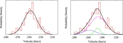
The binned line-of-sight velocity data (red dashed) in Ursa Minor. Right: overplotted is the most probable Gaussian with σ = 11.51 and a |$\overline{{v}}= -247.25$| (black solid) from the null model (single Gaussian component). Left: the line-of-sight velocity distributions of the secondary objects and primary populations. The lines correspond to the velocity dispersions of different populations found with the Bayesian object detection method; velocity offset object (blue dot–dot–space), cold object (green dotted), primary distribution (purple dot–dashed), and the total (black solid). Each component is weighted by its average number of stars found using the Bayesian object detection method. When spatial information is taken into account, the additional kinematic components provide a better fit to the Ursa Minor data.
Before we develop the Bayesian methodology and model comparison methods to show the significance of (or lack thereof), we would like to dissect the data to see if secondary populations are visible as strong local deviations in either mean velocity or velocity dispersion. To this end, we grid a 50 arcmin × 30 arcmin region around the centre of Ursa Minor finely and for each grid point, we find the average velocity |$\overline{{v}}$| and velocity dispersion σ in a 5 arcmin × 5 arcmin bin using the expectation-maximization method (see equations 12b and 13 of Walker et al. 2009a). We disregard grid points where there are fewer than seven stars in the bin. We have plotted the smoothed σ and |$\overline{{v}}$| maps created using this method in Fig. 2. The velocity dispersion map is the upper-left panel and the average velocity map is the upper-right panel. The data are rotated such that the major axis is aligned with the abscissa (θ = 49|$_{.}^{\circ}$|4, see Table 1 for the photometric properties of Ursa Minor we use). There are two interesting features evident: in the σ map, roughly centred at (11 arcmin, −4 arcmin), the σ drops below 6 km s−1 whereas globally, σ = 11.5 km s−1, and in the |$\overline{{v}}$| map centred at ( − 13 arcmin, 6 arcmin), |$\overline{{v}}$| evidently differs from Ursa Minor's overall average (|$\Delta |\overline{{v}}| {>} 10 \: \,\rm{km \: s^{-1}}$|). We have also plotted the number density (lower-left panel) and the positions of the stars (lower-right panel) in Fig. 2 to show the distribution of data and that the kinematic peculiarities are not artefacts due to a low number of stars. The number density map is created the same way as the |$\overline{{v}}$| and σ maps and shows that both features are in regions that are reasonably sampled. In the plot with the positions of the stars, we have also indicated the most probable locations for the centres and the extent of the two features as found by our Bayesian object detection method. We caution the reader that the plotted extents (tidal radii) of these features have large error bars (see Table 2).
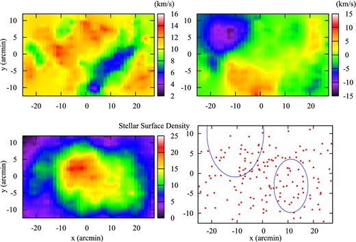
The local kinematics of Ursa Minor using the Muñoz et al. (2005) data set. Upper left: a map of the velocity dispersion of Ursa Minor. A portion of the lower-right quadrant drops below 6 km s−1 while the rest of the galaxy is relatively uniform. Upper right: the average velocity of Ursa Minor found concurrently with the velocity dispersion. In the upper-left quadrant, the deviation |$\Delta \overline{{v}}> 10{\rm -}15 \,\rm{km \: s^{-1}}$| relative to Ursa Minor while the rest of the galaxy does not differ more than 5 km s−1. To make the contour plots, the velocity dispersion and the average velocity were found within a 5 arcmin × 5 arcmin bin (5 arcmin ≃ 110 pc for a distance of 77 kpc). Lower left: the stellar density profile of the stars in the Muñoz et al. (2005) data set. Lower right: the most probable locations and sizes (tidal radii) of the two objects using the Bayesian object detection method in Ursa Minor. Both of these locations correspond to the deviations seen in the average velocity and velocity dispersion maps. The coordinate system used here is such that the x-axis lines up with the major axis which has a position angle of 49|$_{.}^{\circ}$|4 (Kleyna et al. 1998). The adopted centre for Ursa Minor was RA = |$15^{\rm h} 09^{\rm m} 10{.\!\!^{\rm s}}2$|, Dec. = +67°12′52″ (J2000.0) (K03). For the entire sample, we obtain a mean velocity |$\overline{{v}}= -247.25 \,\rm{km \: s^{-1}}$| and velocity dispersion σ = 11.51 km s−1.
The centre of the dip in σ (upper-left panel of Fig. 2) is near the spectroscopic feature found by K03 and the secondary density peak seen in the photometry by several authors (Irwin & Hatzidimitriou 1995; Kleyna et al. 1998; Bellazzini et al. 2002; Palma et al. 2003). The average velocity feature we see does not correspond to any previous noted photometry or kinematic features. However, we note that the stellar isodensity contours of Ursa Minor are significantly asymmetric (Kleyna et al. 1998; Palma et al. 2003) and could hide both features. We now turn to describing our Bayesian object detection method for finding secondary objects and model selection methods for assessing their significance.
2 METHODOLOGY: THEORY
This paper has two primary objectives: to present a statistical methodology for detecting discrete features within a kinematic data set and apply this methodology to the Milky Way satellite galaxy Ursa Minor. In this section, we detail the statistical techniques used to detect kinematic objects within the Ursa Minor data set. The pertinent question we are addressing is whether statistically distinct kinematic objects can be detected within a galaxy's stellar line-of-sight kinematic data and, if such an object is detected, how certain can we be that this object is an actual physical attribute of the system. Thus, we require that any methodology used to detect multiple smaller composite objects within the kinematic data set have two important properties. First, any proposed algorithm must be able to discern an unspecified numbers of statistically separable features within a galaxy's kinematic data set. And secondly, this methodology must allow for some kind of determination of the significance of a proposed object detection.
To calculate the evidence and sample the posterior space, a Bayesian multinested sampling technique was utilized (Skilling 2004; Feroz & Hobson 2008; Feroz, Hobson & Bridges 2009). The nested sampling method calculates the evidence of a model and as a by-product of the computation the posterior is also evaluated. The algorithm transforms the multidimensional evidence integral equation (2), through the ‘prior volume’ X (dX = π(θ)dDθ), into a one-dimensional integral. If the inverse of the prior volume exists and is a monotonically decreasing function of the ‘prior volume’, the evidence integral can be transformed into |$Z = \int _0^1 \mathcal {L}(X){\rm d}X$|. This integral can be evaluated by sampling the likelihood in a decreasing sequence of prior volumes. The multinest algorithm breaks the prior volume into multidimensional ellipsoids which helps sample degenerate parameter spaces and speeds up computation. This sampling algorithm possesses all the capabilities required for this project: multimodal posteriors can be explored efficiently, and the evidence is inherently evaluated (for a more in-depth explanation of the method see Feroz & Hobson 2008; Feroz et al. 2009).
2.1 Likelihood
Parameters, priors, and posteriors. σs and σp are the velocity dispersions of the secondary and primary populations. |$\overline{{v}}_{\rm s}$| and |$\overline{{v}}_{\rm p}$| are the average velocities of the secondary and primary populations. xcen and ycen refer to the x and y centres of the secondary population. Note that the data were rotated such that the x-axis and the major axis are parallel. rtidal is the tidal radius in a top-hat model for the secondary population. Ftotal is the ratio of stars in the secondary population to the total population. For the first section, the 4th and 5th columns denote the values when detecting the two objects individually. The two cuts indicated in the table as ‘Cuts 1 and 2’ are defined as follows. Cut 1 is 0 ≤ σ ≤ 10 km s−1 and |$-252 \le \overline{{v}}\le -242 \,\rm{km \: s^{-1}}$| to find the cold spot object. Cut 2 is 0 ≤ σ ≤ 20 km s−1 and |$-267 \le \overline{{v}}\le -237 \,\rm{km \: s^{-1}}$| to find the velocity offset object. In the second section, the 4th and 5th column denote the values calculated for the two objects simultaneously using a three-component model. The coordinates xcen and ycen of the objects were only allowed to vary within ± 0.1 kpc of the value obtained from the Bayesian object detection method. flocal is the weighted average fraction of secondary population stars in each secondary object's location.
| Parameter | Type | Prior (units) | Cold spot | Velocity offset |
|---|---|---|---|---|
| Model parameters from Bayesian object detection method | ||||
| σs | Flat | Cuts 1/2 (see caption) | |$3.5^{+1.75}_{-2.25}$| | |$8.75^{+1.5}_{-2.25}$| |
| σp | Flat | 0–20 km s−1 | 11.75 ± 0.5 | 10.75 ± 0.5 |
| |$\overline{{v}}_{\rm s}$| | Flat | Cuts 1/2 (see caption) | |$-246.75^{+1.75}_{-2.0}$| | |$-258.75^{+2.0}_{-1.75}$| |
| |$\overline{{v}}_{\rm p}$| | Flat | −242 to −252 km s−1 | −247.5 ± 0.75 | −245.25 ± 0.75 |
| xcen | Flat | −0.6 to 0.6 kpc | |$0.25^{+0.04}_{-0.06}$| | −0.24 ± 0.09 |
| ycen | Flat | −0.4 to 0.4 kpc | |$-0.07^{+0.03}_{-0.07}$| | 0.23 ± 0.02 |
| rtidal | Flat in log10 | 10–300 (pc) | |$151^{+53}_{-28}$| | |$251^{+24}_{-22}$| |
| Ftotal | Flat in log10 | 10−5–1 | |$0.79^{+0.21}_{-0.16}$| | |$0.32^{+0.47}_{-0.26}$| |
| Secondary population model parameters from simultaneous three-component modelling | ||||
| xcen | Flat | −0.24 ± 0.1 kpc | 0.26 ± 0.02 | |$-0.23^{+0.095}_{-0.035}$| |
| ycen | Flat | 0.23 ± 0.1 kpc | −0.07 ± 0.01 | 0.22 ± 0.02 |
| rtidal | Flat in log10 | 10–300 pc | |$151^{+151}_{-10}$| | |$269^{+26}_{-24}$| |
| σs | Flat | Cuts 1/2 (see caption) | 4.25 ± 0.75 | 9.25 ± 1.25 |
| σp | Flat | 0–20 km s−1 | 11.5 ± 0.5 | 11.5 ± 0.5 |
| |$\overline{{v}}_{\rm s}$| | Flat | Cuts 1/2 (see caption) | −246.25 ± 1.0 | −258.0 ± 1.5 |
| |$\overline{{v}}_{\rm p}$| | Flat | −252 to −242 km s−1 | |$-245.25^{+0.75}_{-0.5}$| | |$-245.25^{+0.75}_{-0.5}$| |
| flocal | Derived | - | 70 per cent (15.8/22.5) | 85 per cent (27.0/31.6) |
2.2 Model selection
Even with accurate probability density modelling and thorough parameter space exploration, any object detection methodology will have fairly limited capabilities if the significance of a detection cannot be determined. In this section, we introduce three commonly used model selection techniques to quantitatively derive CL between the multiple component and single component (null model) hypotheses. The techniques used are: the Bayes Factor (B01 or ln B01), a direct calculation of the Kullback–Leibler divergence (DKL) (Kullback & Leibler 1951), and deviance information criterion (DIC; Spiegelhalter et al. 2002).3 For a general review of model selection in cosmology, particularly Bayesian methods, see Liddle, Mukherjee & Parkinson (2006) and Trotta (2008). For a review of the use of information criterion in cosmology, see Takeuchi (2000) and Liddle (2007).
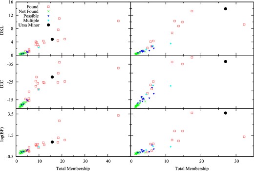
Model selection tests using DKL, DIC, log BF = ln B01 (cf. Section 2.2 for definitions) for 50 mock data sets located at (0.2, −0.1). Also shown for comparison are the results for the actual Ursa Minor data set. A more negative DIC favours the secondary object hypothesis more strongly, while the same is true for larger values of DKL and Bayes factor. Left-hand column: figures in column 1 show the results of the analysis of the mock data sets in exactly the same way as the real data set was analysed to look for the cold object with cuts on mean velocity and dispersion given by 0 ≤ σ ≤ 10 km s−1 and |$-252 \le \overline{{v}}\le -242 \,\rm{km \: s^{-1}}$| (Cut 1). The top panel shows DKL, the middle panel DIC and the bottom panel the logarithm of the Bayes factor (written in the text as ln B01). Mock data sets that had second populations with significant differences in their kinematics with respect to the background population were found with our object detection method. The symbols are labelled/coloured according to whether the x and y posterior is peaked compared to the background around the locations of the secondary populations: peaked/found (red square), not peaked/ not found (green ×), possible peaks (blue triangle) and multiple peaks (light blue diamond). The results for the actual Ursa Minor data set are shown as filled black circle. Right-hand column: this panel has the same symbols and colours as the leftmost column. The difference here is that the velocity cuts used are broader (and the same as that used to find the velocity offset object). The cuts are 0 ≤ σ ≤ 20 km s−1 and |$-267 \le \overline{{v}}\le -237 \,\rm{km \: s^{-1}}$| (Cut 2).
2.3 Testing the method with mock data
We created 100 mock data sets containing a second population to test whether known secondary objects could be detected using our object detection method. The second populations were located at either (0.2, −0.1) or (−0.23, 0.24) kpc (roughly the locations of the cold and velocity offset objects). The kinematic and structural parameters of this second population were selected to mimic the cold and velocity offset objects. The positions and velocity errors from the Ursa Minor data set were used to simulate observational errors. To pick which population a star is assigned to, the local fraction was found via equation (8) and membership was randomly assigned with the second population weighted by the local fraction. The primary population parameters were the best-fitting values from Ursa Minor photometry and the kinematics of the entire sample: rtidal = 1.745 kpc, rcore = 0.401 kpc, ellipticity ϵp = 0.56, σ = 11.5 km s−1, and |$\overline{{v}}= -247 \,\rm{km \: s^{-1}}$|. The second population's base parameters were: ϵs = 0, θs = 0.0, Ftotal = 60/212, rcore = 0.05 kpc, |$\Delta \overline{{v}}_{\rm s} = 0 \,\rm{km \: s^{-1}}$|, σ = 4 km s−1, rtidal = 0.15 kpc for (0.2, −0.1) location. For the (−0.23, 0.24) location, we used a slightly larger value for tidal radius, rtidal = 0.25 kpc. We note that both populations were created assuming an underlying King profile but the object detection used a top-hat model when finding the second population, identically to how the objects were found in the actual data. Each individual mock data set had 1–3 secondary parameters that deviated from the base parameters to test how each parameter affected the detection. In some sets, we did not expect to find the secondary population, for example, if they had small tidal radius or small secondary population fraction.
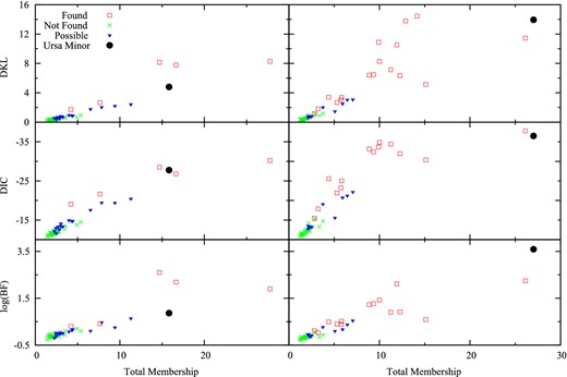
The results for model selection of the DKL, DIC, ln B01, and total membership using two different kinematic priors are summarized in Fig. 3 (secondary population located at (0.2, −0.1)) and Fig. 4 (secondary population located at (−0.23, 0.24)). In both figures, the two columns show different kinematic priors with the left-hand column showing the cuts to find kinematically cold objects (0 ≤ σ ≤ 10 km s−1, |$-252 \le \overline{{v}}\le -242 \,\rm{km \: s^{-1}}$|) and the right-hand column has the cuts to find objects with a significant velocity offset (0 ≤ σ ≤ 20 km s−1, |$-267 \le \overline{{v}}\le -237 \,\rm{km \: s^{-1}}$|); this cut will also find the kinematically cold objects, but in the Ursa Minor case the velocity offset object was significantly more likely and tended to dominate the posterior. The symbols for these columns are labelled/coloured according to whether the x and y posterior was peaked (compared to the back ground) around the location of the secondary population: peaked/‘found’ (red square), not peaked/‘not found’ (green ×), ‘possible’ peaks (blue triangle), double peaked with one correct (light blue diamond). Results for the actual Ursa Minor data with corresponding cuts are shown as filled black circle. The ‘possible’ peaks are posteriors where there was a peak near the second population's centre, a small/medium peak somewhere else in the posterior, or a small peak at the correct location. The double peaked data had one peak at the correct location and a second at another location. The ‘possible’ sets tended to span the border between ‘found’ and ‘not found’ and were not easily categorized otherwise. This definition of ‘found’/‘not found’ corresponds to higher likelihood values at the locations of secondary populations (similar to the K03 method).
Both figures show a clear trend between the ‘found’ and ‘not found’ sets in all the model selection methods. Note that more negative DIC corresponds to favouring the more complicated model. Sets that are ‘not found’ by the object detection have model selection criteria that is equivalent to the model selection criteria of null hypothesis mock data sets (i.e. sets made with no second population), cf. Section 3.1. Most importantly, the model selection criteria for the two objects found in Ursa Minor data also lie in the ‘found’ section of the mock data's selection criteria. From the analysis of these mock data sets, we conclude that our method is fully capable of detecting the cold and velocity offset, and the model selection criteria favour the presence of two additional components in Ursa Minor.
3 RESULTS
We have found two objects in the Ursa Minor data set of Muñoz et al. (2005) using a Bayesian object detection method. The first object, referred to as the ‘cold object’ here, is kinematically cold, |$\sigma _{\rm cold} = 3.5^{+1.8}_{-2.3} \rm \,\rm{km \: s^{-1}}$|, with an average velocity close to that of the full Ursa Minor sample, |$\overline{{v}}_{\rm cold} = -246.8^{+1.8}_{-2.0} \,\rm{km \: s^{-1}}$|. The location coincides with the location of the K03 stellar clump. The second object, referred to as the velocity offset object, has a large average velocity offset compared to the mean velocity of Ursa Minor, |$\overline{{v}}_{\rm vo} = -258.8^{+2.0}_{-1.8} \,\rm{km \: s^{-1}}$| with a dispersion of |$\sigma _{\rm vo} = 8.8^{+1.5}_{-2.3} \,\rm{km \: s^{-1}}$|. The kinematics and structural properties are summarized in the first section of Table 2. The model selection tests for the cold object are: Total Membership = 15.8, DKL = 4.8, DIC = −26.1, ln B01 = 0.9. The model selection tests for the velocity offsets object are: Total Membership = 27.0, DKL = 13.9, DIC = −36.5, ln B01 = 3.6. In Figs 3 and 4, the results of model selection test are plotted alongside the mock set distributions (filled black dot). All of the model selections tests favour the additional secondary objects with moderate to high significance except for the Bayes factor which has weak to moderate significance for the cold and velocity offset objects.4 This significance is based on the recommendations of Trotta (2008), Ghosh, Delampday & Samanta (2006) and Spiegelhalter et al. (2002). However, it is important to judge the significance of the information criteria and the Bayes factor for the problem at hand. We do this by generating null data sets and deriving the information criteria and Bayes factor in the same way as the real data are handled. When this test is performed, we find that the CL of both objects are above the 98 per cent CL (see Table 2). In addition, all of the model selection values, for both locations/objects, lie in the ‘found’ region of the mock sets of Figs 3 and 4.
3.1 Significance of information criteria and Bayes’ factor
In order to assess the significance of the model selection tests, knowledge of the false positive rate is helpful. We make use of two types of tests for false positives: null hypothesis mock data sets and scrambled data sets. Null hypothesis mock data sets are constructed by redrawing the line-of-sight velocities from a Gaussian with Ursa Minor kinematics.5 To simulate positional and velocity errors, the positions of stars and the line-of-sight velocity errors were kept. The scrambled sets were constructed by repicking a random observed line-of-sight velocity and line-of-sight velocity error pair, without replacement, for each star in the data set. 1000 null hypothesis mock data sets and scrambled data sets were constructed and analysed with our object detection method.
The results of the object detection method and our employed model selection tests for the null hypothesis mock data sets and the scrambled mock data sets are shown in Fig. 5. The top and bottom rows refer to the null hypothesis and scrambled tests, respectively. The DKL (right-hand column), DIC (middle column), and ln B01 (left-hand column) are binned and the maximum is normalized to unity. The analysis with the cuts to find cold objects (0 ≤ σ ≤ 10 km s−1, |$-252 \le \overline{{v}}\le -242 \,\rm{km \: s^{-1}}$|) is shown in red, while that with cuts to find objects with significant velocity offset (0 ≤ σ ≤ 20 km s−1, |$-267 \le \overline{{v}}\le -237 \,\rm{km \: s^{-1}}$|) is shown in blue. The model selection results for the real Ursa Minor data are plotted as vertical lines: cold object with green dotted line and velocity offset object with purple dash–dotted line. The CL of the model selection criteria for the null hypothesis mock data sets and scrambled data sets are above the 98.5 per cent CL with every model selection criteria. They are summarized in Table 3. Even though the ln B01 shows weak evidence for the cold object according to standard definitions, it is still above the 95 per cent CL for both the null hypothesis mock data sets and scrambled data sets.
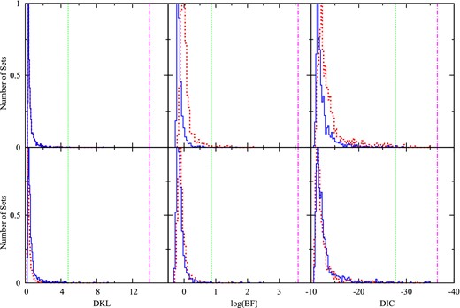
Histograms of DKL, DIC, and Bayes factor from analyses of 1000 null hypothesis mock data (top rows) and 1000 scrambled data sets (bottom rows) with Cut 1 (red dotted) and Cut 2 (blue solid). The vertical lines show the DKL, DIC, and Bayes factor values for the actual Ursa Minor data set with Cut 1 (green dotted) and Cut 2 (magenta dot–dashed). The inferred CL for the Ursa Minor data is ≥98.5 per cent for all tests.
CL computed from null hypothesis and scrambled mock data sets. The inferred CL refers to the number of null hypothesis mock data sets and scrambled data sets that have a model selection value lower than that of the actual Ursa Minor data. The 95 per cent CL value is defined such that 95 per cent of the null hypothesis or scrambled data sets have a value below this. Both additional populations found in the Ursa Minor data are above the 98 per cent CL for all the model selection methods. The two cuts indicated in the table as ‘Cuts 1 and 2’ are defined as follows. Cut 1 is 0 ≤ σ ≤ 10 km s−1 and |$-252 \le \overline{{v}}\le -242 \,\rm{km \: s^{-1}}$| used to find the cold spot object in the data. Cut 2 is 0 ≤ σ ≤ 20 km s−1 and |$-267 \le \overline{{v}}\le -237 \,\rm{km \: s^{-1}}$| used to find the velocity offset object in the data.
| Test using null hypothesis mock data sets | ||||
|---|---|---|---|---|
| Total average | Information entropy | Bayesian evidence | ||
| membership | DKL | DIC | ln B01 | |
| Value at 95 per cent CL from null hypothesis mock data sets using Cut 1 | 5.25 | 1.28 | −16.35 | 0.17 |
| Cold object values from data (inferred CL) | 15.82 (99.8 per cent) | 4.82 (99.7 per cent) | −26.08 (99.5 per cent) | 0.87 (99.7 per cent) |
| Value at 95 per cent CL from null hypothesis mock data sets using Cut 2 | 4.49 | 1.84 | −17.79 | 0.13 |
| Velocity offset object values from data (inferred CL) | 27.02 (>99.9 per cent) | 13.93 (>99.9 per cent) | −36.49 (99.9 per cent) | 3.59 (>99.9 per cent) |
| Test using scrambled data sets | ||||
| Total average | Information entropy | Bayesian evidence | ||
| membership | DKL | DIC | ln B01 | |
| Value at 95 per cent CL from scrambled mock data sets using Cut 1 | 6.99 | 2.22 | −20.45 | 0.40 |
| Cold object values from data (inferred CL) | 15.82 (99.7 per cent) | 4.82 (99.1 per cent) | −26.08 (98.5 per cent) | 0.87 (99.0 per cent) |
| Value at 95 per cent CL from scrambled mock data sets using Cut 2 | 3.89 | 1.46 | −16.30 | 0.07 |
| Velocity offset object values from data (inferred CL) | 27.02 (>99.9 per cent) | 13.93 (>99.9 per cent) | −36.49 (>99.9 per cent) | 3.59 (>99.9 per cent) |
3.2 Narrowing down secondary population parameters using a three-component model
In the detection phase, the kinematic properties of one object are determined while the other is part of the background. To reliably calculate the kinematic properties of each secondary object, we introduce a model with two secondary populations fixed within 0.1 kpc from the best-fitting centre locations. Equation (7) is modified to include a third component. Two normalization parameters are required, |$\alpha _2 = \frac{N_2}{N_1}$|, and |$\alpha _{\rm p} = \frac{N_{\rm p}}{N_1}$| where N1 and N2 denote the normalization of the first and second object. The results for the kinematic parameters are: σcold = 4.3 ± 0.8 km s−1, |$\overline{{v}}_{\rm cold} = -246.3 \pm 1.0 \,\rm{km \: s^{-1}}$|, σvo = 9.3 ± 1.3 km s−1, and |$\overline{{v}}_{\rm vo} = -258.0 \pm 1.5 \,\rm{km \: s^{-1}}$|, respectively. These values are in full agreement with the values obtained using the two-component (Bayesian object detection) method.
The normalization ratios, as defined, are not easily interpreted. So we introduce a derived parameter, local fraction or flocal, that is defined as the weighted average of stars with memberships greater than 50 per cent in the secondary population compared to the total number of stars within the secondary object's tidal radius. In short, it is a measure of the fraction of secondary stars in each object's location. We derive flocal, cold = 15.8/22.5 or 70 per cent and flocal, vo = 27.0/31.6 or 85 per cent. Clearly, we are able to find these objects only because they seem to have a high local fraction. The kinematics and structural properties of the secondary population model are summarized in the second section of Table 2. In upper-left and -right panels of Fig. 6, we have plotted the posteriors for the x and y centres, respectively, for the cold (black solid) and velocity offset objects (red dotted). The centres for the cold and velocity offset object are (0.25, −0.07) kpc and ( + 0.24, 0.23) kpc and the two panels show the deviation from the ‘fixed’ centres. The lower-right (lower-left) panel of Fig. 6 is the posterior of the σs (|$\overline{{v}}_{\rm s}$|) for the cold (black solid), velocity offset objects (red dotted), and primary (blue dashed). The Bayes factor of this model is 10.0. The three-component model is highly favoured compared to the null model.
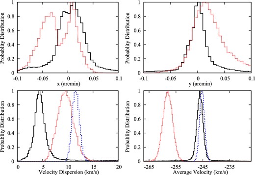
The posteriors for the secondary populations in Ursa Minor using the three-parameter model. The secondary populations are fixed at (0.25, −0.07)kpc and ( + 0.24, 0.23)kpc and allowed to vary 0.1 kpc in both coordinates. They correspond to the cold (black solid) and the velocity offset (red dots) objects, respectively. Upper left: the x coordinate posteriors for of the secondary populations. Upper right: the y coordinate posteriors for the secondary populations. Lower left: the velocity dispersion posteriors of the cold object (black solid), velocity offset object (red dotted), and the primary (blue dashed). Lower right: the average velocity posteriors of the cold object (black solid), velocity offset object (red dotted), and the primary (blue dashed). The secondary populations have distinct kinematic properties and are both localized.
An increased prior volume for the centres and tidal radius in the three-component model changes the posteriors for the structural parameters of the velocity offset object but does not change its kinematics. By only allowing more freedom in the location of the centres (200 pc versus 100 pc), the posteriors of both centres gain tails. An increase in the maximum tidal radius (in the prior) of the objects (500 pc from 300 pc) increases the size of the velocity offset object, and moves its centre roughly 150 pc away from the centre of Ursa Minor while the same change introduces tails in the posterior of the cold object. This change is from several stars in the outer region of Ursa Minor that have consistent kinematics with the velocity offset object. Given these results, it is fair to say that the size and centre of the secondary objects are not known with high precision and more data will help considerably. However, our conclusions regarding kinematics seem to be robust.
3.3 Perspective motion
To investigate this issue further, we run a three-component model to detect the two secondary objects when including perspective motion. We add this effect into our likelihood function by changing the model velocity for all three components (cf. |$\overline{v}_{\rm p, s}$| in equation 4) to vlos, i given by equation (13) with xi and yi for each star measured from the centre of Ursa Minor. Each component has its own vz, but vx and vy are the same for all three components. Note that the actual tangential velocity of the two secondary components is now implicitly tied to the vz value – there is no hope of disentangling them given the small projection on the sky of the secondary components. We then impose the same constraints on the centre as before (cf. Section 3.2). We find results that are consistent with those we found in Section 3.2 in the absence of perspective motion: |$x_{\rm cold} = 0.245^{+0.03}_{-0.04} \,\rm kpc$|, |$y_{\rm cold} = -0.065^{+0.015}_{-0.025} \,\rm kpc$|, and |$x_{\rm vo} = -0.275^{+0.04}_{-0.035} \,\rm kpc$|, yvo = 0.24 ± 0.025 kpc. The kinematic properties are the same as without perspective motion except with larger error bars. Thus, the three-component model with the prior on the centres provides a different fit and favours the presence of the secondary objects over perspective motion. Had perspective motion or a velocity gradient or rotation been a better fit to the likelihood instead of either of the objects, this would not have been the case since the likelihood allows for the freedom to dial down the fraction of stars in the secondary objects. In this three-component fit, the mean velocity of Ursa Minor is |$(-311 \pm 212,-548^{+357}_{-324},-245.5 \pm 0.75) \,\rm{km \: s^{-1}}$|, in good agreement with the results obtained when stars in the locations populated by the secondary populations are removed.
We also explored the effect of using the Bayesian object detection method with perspective motion. This could lead to faulty results (and we show below that it does) because the velocity offset spot has a large impact on the determination of the background parameters – specifically the perspective motion. With the velocity cuts to find the cold object, we find a mean velocity for Ursa Minor of |$(-100^{+100}_{-100}, -1125^{+275}_{-250},-247.5^{+0.5}_{-0.5}) \,\rm{km \: s^{-1}}$| and a dispersion in the line-of-sight velocity of 11.0 ± 0.5 km s−1. The dispersion of the cold object is now consistent with zero at about 1σ, 3.25 ± 3.0 km s−1 and the location of the centres is now much less well determined. However, the values obtained for the perspective motion are unphysically large, and hence, this is clearly not the correct model to be considered. With the ±20 km s−1 velocity cut (to find the velocity offset object), we find a mean velocity for Ursa Minor of |$(-200^{+150}_{-150}, -1175^{+400}_{-400}, -247^{+1.0}_{-1.25}) \,\rm{km \: s^{-1}}$| and 10.75 ± 0.5 km s−1 for its dispersion in the line-of-sight velocity. The centre, as with the other object, is no longer tightly constrained, and the hint for deviation in mean velocity for this object is muted (|$-258^{+7.5}_{-4.5} \,\rm{km \: s^{-1}}$|). Thus, we arrive at the conclusion (unsurprisingly) that varying background parameters in Bayesian object detection methods can lead to faulty results in data sets containing multiple signals if those signals have a significant effect on the determination of the background parameters. In particular, for this analysis we saw that the presence of the velocity offset spot affects the magnitude and the direction of the inferred tangential motion and hence the object detection method has trouble fitting one secondary location and perspective motion. But with two localized secondary populations and perspective motion the method still picks out both secondary objects. Thus, the three component model is preferred by this data set.
A tangential velocity measured using perspective motion could also be hiding a possible solid-body rotation. An order of magnitude estimate of this rotation speed would be |$v_{\rm rot} = \frac{R_{\rm e}}{D} \scriptstyle\sqrt{v_x^2 + v_y^2}\:$| (|$R_{\rm e} = 445 \pm 44 \: \rm{pc}, D = 77 \pm 4 \: \rm{kpc}$|). Using the results presented in this section, we calculate vrot ∼ 7 km s−1 with entire data set, and vrot ∼ 4 km s−1 when the velocity offset population is removed, and when both secondary populations are removed or when all stars near the secondary populations are removed. The rotation speeds are all comparable but in each estimate the rotation is about a different axis. The summary of our results from this section is that a larger data set is required to simultaneously constrain properties of the secondary populations and rotation or proper motion. The results of our three-component analysis suggest that the data prefer the presence of both secondary objects to perspective motion (or a rotation that masquerades as it).
4 DISCUSSION
We discuss how our results compare to previous work and possible explanations for our results. K03 utilized a likelihood test comparing two (Ursa Minor dSph plus a secondary population) and one component kinematic models to estimate the locations of secondary populations and to find the best-fitting parameters of the secondary populations. They discovered a stellar clump (a likelihood ratio of ∼104) located at (10 arcmin, 4 arcmin) (on-sky frame relative to the Ursa Minor centre) with kinematic parameters, σ = 0.5 km s−1, vs = −1 km s− 1, and clump fraction of 0.7 (fraction of stars in the second population). The kinematically cold object found with our object detection method is centred at (10.8 arcmin ± 1.8, 5.5 arcmin ± 0.9) (on-sky frame relative to Ursa Minor centre), has a size of 6.7 arcmin ± 0.5, with kinematic properties σ = 4.25 ± 0.75 km s−1, and |$\Delta \overline{{v}}= -1.1^{+1.5}_{-1.25} \,\rm{km \: s^{-1}}$|. The difference between our results and those of K03 lie in the velocity dispersion of the cold object. We have considerably more stars (in total 212 to 134 of K03) and are therefore able to infer the dispersion with much greater confidence. We find the mean value for the velocity dispersion to be close to 4 km s−1, similar to the dispersion of Segue 1 dSph (Simon et al. 2011). In addition, our methodology allows us to compute error bars on model parameters.
The main uncertainty in our estimates of the dispersion for cold and velocity offset objects is the presence of perspective motion or solid-body rotation. Perspective motion by itself cannot explain these secondary populations. A three-component analysis (i.e. main Ursa Minor population and both secondary populations) with the coordinates of the centres fixed to within 100 pc and including perspective motion (with unconstrained tangential velocity) prefers the presence of both the secondary populations. In this analysis, the velocity dispersions of the cold or velocity offset objects are not significantly different from the values obtained without including perspective motion.
To estimate the luminosity of the secondary objects, we use the total membership of the objects with the assumption that the stars were drawn uniformly from the three distributions of Ursa Minor. We find the luminosity of the cold and velocity offset objects to be 4 × 10⁴ and 6 × 10⁴ L⊙. The luminosity of the K03 object is 1.5 × 10⁴ L⊙, and given the uncertainties we would chalk this down as agreement between the two analyses. The dynamical mass within half-light radius of dispersion supported systems can be estimated to about 20 per cent accuracy using the line-of-sight velocity dispersions and the half-light radius (Walker et al. 2009b; Wolf et al. 2010). Assuming that the ratio of r1/2/rtidal of the objects is the same as that of Ursa Minor, we find M1/2 = 6 × 10⁵ M⊙, and M1/2 = 5 × 10⁶ M⊙ for the cold and velocity offset object. From this, M/L(r1/2) ≈ 30 M⊙/L⊙ and M/L(r1/2) ≈ 175 M⊙/L⊙ for the cold and velocity offset objects. If we use this same estimator to find the velocity dispersions assuming the objects are relaxed systems with only stellar components and M/L = 2 (as in K03), we estimate a velocity dispersion of σ = 1.0 km s−1 for both the cold and velocity offset objects. This differs from the velocity dispersion found through our object detection method by 4σ and 6.6σ for the cold and velocity offset objects, respectively. Note that the estimator for M1/2 assumes that the system is dynamical equilibrium, which may not be the case here. If our current results hold up with the addition of more data, then either these objects have highly inflated velocity dispersions due to the influence of motion in binary stellar systems or tidal disruption, or these objects really do have a much larger mass than inferred from their luminosities. In the latter case, we would have found a satellite of Ursa Minor, the first detection of a satellite of a satellite galaxy. We discuss each of these possibilities briefly below.
Contribution of binary orbital motion to the line-of-sight velocities can inflate the observed line-of-sight velocities of stars (Aaronson & Olszewski 1987; Hargreaves, Gilmore & Annan 1996; Olszewski, Pryor & Armandroff 1996; McConnachie & Côté 2010; Minor et al. 2010). A galaxy with a lower intrinsic velocity dispersion has a higher chance of having its observed dispersion inflated. A dSph with a velocity dispersion between 4 and 10 km s−1 is highly unlikely to be inflated by more than 30 per cent (Minor et al. 2010, for an application of this method see Simon et al. 2011, Martinez et al. 2011). The objects we found have observed velocity dispersions in this range. Assuming both objects are inflated by 30 per cent, their actual intrinsic velocity dispersion would be between 2.5-3.3 km s− 1 and 7.1 km s−1, respectively, for the cold and velocity offset objects. These velocity dispersions are still much higher than 1 km s−1 (that is expected for a relaxed stellar system, i.e. a globular cluster). It is unlikely that binary orbital motion alone can account for the large velocity dispersions inferred from this data set for both secondary populations. With multi-epoch data, we will be able test this hypothesis directly as was done for Segue 1 dSph (Martinez et al. 2011).
To assess the effect of tidal disruption from Ursa Minor, we calculate the Jacobi Radius, rJ, and compare rJ to the mean tidal radius estimated from our three-component analysis. To calculate the Jacobi radius, we consider both an NFW (Navarro et al. 1997) and a pseudo-isothermal (cored) profile for the halo of Ursa Minor. To set the NFW density profile of Ursa Minor, we pick NFW scale radius rs = 1 kpc and estimate the density normalization ρs using M1/2 values from Wolf et al. (2010) for an NFW profile. We find that if the actual distance of the centre of the objects is equal to the projected distance from the centre of Ursa Minor, then rJ < rt. If the objects are further than about 1 kpc away, then rJ > rt with the NFW profile. The situation for a pseudo-isothermal profile (|$1/(r^2+r_0^2)$|) with r0 = 300 pc is similar, with rJ > rt if the objects are further than about 1–2 kpc from the centre of Ursa Minor. The rJ estimates indicate that tides from Ursa Minor could have an effect on these objects even if they are protected by their own dark matter haloes. The survival of globular cluster sized objects in dSphs has far-reaching implications for the density profile of the host halo (K03; Goerdt et al. 2006; Strigari et al. 2006; Cowsik et al. 2009; Lora et al. 2012). The objects we find are more extended and massive than the globular cluster sized objects considered in such work in the past. Thus, these constraints will have to reevaluated.
Generically, the estimated high dispersions of these objects and their survival are facts at odds with each other. The age of Ursa Minor ( ∼ 12 Gyr) is much longer than the crossing time for stars inside Ursa Minor of ∼ 150 Myr (assuming a typical velocity of 10 km s−1). The crossing times for the stars in the cold and velocity offset object are ∼ 50 Myr. These objects have had time to make multiple orbits around Ursa Minor, and it is hard to see how they could have survived given the short crossing times unless they have been recently captured by Ursa Minor and are now in the process of tidal disruption (which would account for the inflated velocity dispersion). However, this is not a likely scenario since Ursa Minor probably fell into the Milky Way early, between 8 and 11 Gyr (Rocha, Peter & Bullock 2012), and capturing a large object after that is unlikely. It is more reasonable to assume that these objects have survived for long because they were protected by a dark matter halo of their own. The reality is probably more complicated: these objects may have their own dark matter haloes and at the same time are being tidally disrupted. These implications are intimately tied to the dark matter halo of Ursa Minor and pinning down the properties of these objects would help to decipher if the dark matter halo of Ursa Minor has a cusp or a core.
5 CONCLUSION
We have presented a method for finding multiple localized kinematically-distinct populations (stellar substructure) in line-of-sight velocity data. In the nearby dwarf spheroidal galaxy Ursa Minor, we have found two secondary populations: ‘cold’ and ‘velocity offset (vo)’ objects. The estimated velocity dispersions are σcold = 4.25 ± 0.75 km s−1 and σvo = 9.25 ± 1.25 km s−1, and the estimated mean velocities are |$\overline{{v}}_{\rm cold} = -246.25 \pm 1.0 \: \,\rm{km \: s^{-1}}$| and |$\overline{{v}}_{\rm vo} = -258.0 \pm 1.5 \: \,\rm{km \: s^{-1}}$|. They are located at |$(0.25_{-0.06}^{+0.04}, -0.07_{-0.07}^{+0.03})\ \rm kpc$| (cold object) and ( − 0.24 ± 0.09, 0.23 ± 0.02) kpc (velocity offset object) with respect to the centre of Ursa Minor. The location of the cold object matches that found earlier by K03, but our results reveal that the velocity dispersion of this cold object could be large with a mean value close to 4 km s−1. To assess the significance of our detections, we employed the Bayes factor and information criteria DKL and DIC supplemented with the analysis of mock data sets with secondary populations, null hypothesis mock data sets and scrambled data sets. The two secondary objects have >98.5 per cent CL in all the model selection tests employed.
If the velocity dispersions are as large as our Bayesian analysis seems to indicate, then these objects are likely undergoing tidal disruption or are embedded in a dark matter halo. The two possibilities are not exclusive of each other. If these objects are dark matter dominated, this would be the first detection of a satellite galaxy.
As emphasized by K03, the presence of localized substructure has important implications for inner density profile of the dark matter halo of Ursa Minor. The shape of the inner profile (cusp or core) has important implications for the properties of the dark matter particle with cold dark matter model predicting a cuspy inner density profile. If the stellar substructure is hosted by its own dark matter halo, then it has further implications for dark matter models since this would likely be the smallest bound dark matter structure discovered.
This research was supported in part by the National Science Foundation Grant 0855462 at UC Irvine. This research was supported in part by the Perimeter Institute of Theoretical Physics during a visit by MK. Research at Perimeter Institute is supported by the Government of Canada through Industry Canada and by the Province of Ontario through the Ministry of Economic Development and Innovation. GDM acknowledges support from the Wenner-Gren Foundations. RRM acknowledges support from the GEMINI-CONICYT Fund, allocated to the project no. 32080010, from CONICYT through project BASAL PFB-06, and the Fondo Nacional de Investigación Científica y Tecnológica (Fondecyt project no. 1120013).
We also tried a constant fraction within the location of the second population. In all three parametrizations of α, the same objects are found.
Additional stellar profiles were used for the secondary population including a King and Plummer profile. Both objects were still detected. The scale radii for the King and Plummer stellar profiles were unconstrained.
Two other common information criterion are the Akaike information criterion (AIC; Akaike 1974) and the Bayesian information criterion. These information criterion are Gaussian approximations to the DKL and Bayes factor, respectively. We do not use these as we have a direct calculation of them.
Assuming a uniform prior on the tidal radius of the objects instead of a prior in log10 increases the B01 to 1.4 and 5.7 for the cold and velocity offset spots, respectively.
We used |$\overline{{v}}= -247.0 \,\rm{km \: s^{-1}}$| and σ = 11.5 km s−1.
