-
PDF
- Split View
-
Views
-
Cite
Cite
O. G. King, D. Blinov, A. N. Ramaprakash, I. Myserlis, E. Angelakis, M. Baloković, R. Feiler, L. Fuhrmann, T. Hovatta, P. Khodade, A. Kougentakis, N. Kylafis, A. Kus, D. Modi, E. Paleologou, G. Panopoulou, I. Papadakis, I. Papamastorakis, G. Paterakis, V. Pavlidou, B. Pazderska, E. Pazderski, T. J. Pearson, C. Rajarshi, A. C. S. Readhead, P. Reig, A. Steiakaki, K. Tassis, J. A. Zensus, The RoboPol pipeline and control system, Monthly Notices of the Royal Astronomical Society, Volume 442, Issue 2, 1 August 2014, Pages 1706–1717, https://doi.org/10.1093/mnras/stu176
Close - Share Icon Share
Abstract
We describe the data reduction pipeline and control system for the RoboPol project. The RoboPol project is monitoring the optical R-band magnitude and linear polarization of a large sample of active galactic nuclei that is dominated by blazars. The pipeline calibrates and reduces each exposure frame, producing a measurement of the magnitude and linear polarization of every source in the 13 arcmin × 13 arcmin field of view. The control system combines a dynamic scheduler, real-time data reduction, and telescope automation to allow high-efficiency unassisted observations.
1 INTRODUCTION
The RoboPol project1 is monitoring the R-band optical linear polarization and magnitude of a large sample of active galactic nuclei (AGN). The statistically well-defined sample is drawn from gamma-ray-loud AGN detected by Fermi (Abdo et al. 2010a; Nolan et al. 2012) and is dominated by blazars, as described in Pavlidou et al. (in preparation). The main science goal of the RoboPol project is to understand the link in AGN between optical polarization behaviour, particularly that of the electric vector position angle (EVPA; e.g. Marscher et al. 2008; Abdo et al. 2010b), and flares in gamma-ray emission.
The RoboPol polarimeter (Ramaprakesh et al., in preparation) is an imaging photopolarimeter that measures the linear polarization and magnitude of all sources in the 13 arcmin × 13 arcmin field of view. It is installed on the 1.3-m telescope at the Skinakas Observatory2 in Crete, Greece. The large amount of observing time (four nights a week on average over the Skinakas 9-month observing season) and long duration of the project (at least three years) will generate a large amount of data, requiring a fully automated data reduction pipeline and observing procedure. While the RoboPol instrument is optimized for operation in the R band, it can also observe in the I and V bands. All observations described in this paper were made with a Johnson–Cousins R-band filter.
Blazar emission at optical wavelengths is highly variable and the optical polarization events we aim to characterize can occur very rapidly. This requires a flexible observing scheme capable of responding to changes in the optical polarization of a source without human intervention. In this paper, we describe the data reduction pipeline and control system developed to meet these requirements. It is organized as follows. The telescope and instrument are described in Section 2. The data reduction pipeline and its performance are described in Section 3, and the control system is described in Section 4. We conclude in Section 5.
2 TELESCOPE AND INSTRUMENT
2.1 Telescope
The 1.3-m telescope at the Skinakas Observatory (1750 m, 23°53′57″E, 35°12′43″N) has a modified Ritchey–Chrétien optical system (129 cm primary, 45 cm secondary, f/7.54). It has an equatorial mount, built by DFM Engineering3, with an off-axis guiding system. The telescope is equipped with several other instruments in addition to the RoboPol polarimeter, including an imaging camera, IR camera, and spectrograph.
Control of the telescope and its subsystems is spread over several computers. The guiding camera, its focus control, the RoboPol filter wheel, and the RoboPol CCD camera are connected directly to the main control computer. The secondary mirror focus control, the dome control, and the equatorial mount control are connected to the telescope control system (TCS) computer, which interfaces with the main control computer through a serial link. A third computer monitors the weather station.
2.2 Instrument
The RoboPol instrument (Ramaprakesh et al., in preparation) is a 4-channel imaging photopolarimeter designed with high observing efficiency and automated operation as prime goals. It has no moving parts other than a filter wheel. Instead, as shown in Fig. 1, the instrument splits the pupil in two – each half incident on a half-wave retarder followed by a Wollaston prism (WP). One prism is oriented such that it splits the rays falling on it in the horizontal plane (blue prism and rays in Fig. 1), while the other prism's orientation splits them in the vertical plane (red in Fig. 1).
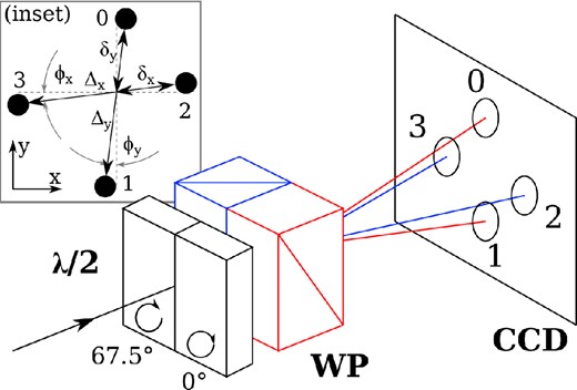
Diagram showing the basic operation of the RoboPol instrument. The pupil of the instrument is split in two, each half incident on a half-wave retarder followed by a Wollaston prism, labelled λ/2 and WP, respectively, with differing fast axis and prism orientations as indicated. The blue pair splits the rays horizontally to produce the spots labelled 2 and 3, while the red pair produces the vertical spots 0 and 1. The linear polarization parameters are then calculated using equation (1). Inset: the pattern of spots at each position on the CCD is described by this model. The distance between the spots Δx and Δy, their distance from the intersection point δx and δy, and their angle with respect to the CCD axes ϕx and ϕy all vary independently across the field.
Every point in the sky is thereby projected to four points on the CCD. The fast axis of the half-wave retarder in front of the first prism is rotated by 67|$_{.}^{\circ}$|5 with respect to the other retarder. In the instrument reference frame, the horizontal channel measures the u = U/I fractional Stokes parameter, while the vertical channel measures the q = Q/I fractional Stokes parameter, simultaneously, with a single exposure. This design eliminates the need for multiple exposures with different half-wave plate positions, thereby avoiding systematic and random errors due to sky changes between measurements and imperfect alignment of rotating optical elements.
The instrument has a large 13 arcmin × 13 arcmin field of view that enables relative photometry using standard catalogue sources and the rapid polarimetric mapping of compact sources in large sky areas. While the instrument is designed to operate in the optical V, R, and I-bands, RoboPol monitoring observations are generally made using a Johnson–Cousins R-band filter. An example of an image from the instrument is shown in Fig. 2 .
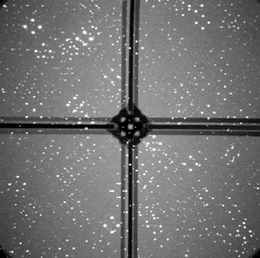
An example of a RoboPol image. Each point in the sky has been mapped to four spots on the CCD. A focal plane mask, held in place by four support legs, reduces the sky background level for the central target.
The primary scientific goal of the project is to monitor the linear polarization of blazars, which appear as point sources at optical wavelengths, so we optimized the instrument sensitivity for a source at the centre of the field by using a mask in the telescope focal plane. The focal plane mask has a cross-shaped aperture in the centre where the target source is placed. The focal plane area immediately surrounding this aperture is blocked by the mask. This prevents unwanted photons from the nearby sky and sources from overlapping with the central target spots on the CCD, increasing the sensitivity of the instrument for the central source. The sky background level surrounding the central target spots is reduced by a factor of 4 compared to the field sources. The focal plane mask and its supports obscure part of the field, reducing the effective field of view.
The polarimeter is attached to an Andor DW436 CCD camera which has an array of 2048 × 2048 pixels and can be cooled to −70°C where it has negligible dark noise (<0.001 e− pixel−1 s−1).
2.2.1 Model of the instrument
Inspection of Fig. 2 reveals that the pattern of four spots on the CCD corresponding to a source is dependent on the location of the source in the field. This is expected, and is due to optical distortions in the instrument. In addition to this geometric spot-pattern effect, there are systematic errors that affect the intensity in each spot. For an unpolarized source, the number of photons falling on each spot should be equal. However, unavoidable imperfections in the optics result in deviations of the ratios N0/N1 and N2/N3 from 1, and N0 + N1 ≠ N2 + N3.
The model also predicts the pattern that the spots make on the CCD. As shown in Fig. 1, we model the distance between the spots Δx and Δy, the angle between the spots and the CCD axes ϕx and ϕy, and the distance of the spots from the intersection of their joining lines δx and δy. This is modelled at every point in the field, and is used by the pipeline to identify which spots correspond to which astronomical source. To produce the model, we take multiple exposures of an unpolarized standard star at many locations in the field and map the variation in the non-ideal behaviour. We fit the model to the measured spot pattern and intensities and save the model coefficients to disc for use by the data reduction pipeline. We re-fit the model parameters each time the instrument is removed and replaced.
3 PIPELINE
3.1 Overview
The RoboPol pipeline measures the magnitude and linear polarization of every unobscured source in the field, i.e. every source that is not obscured by the focal plane mask and its supports. A flow-diagram of the pipeline is shown in Fig. 3. The pipeline is written in python, with some subroutines written in cython4 to improve the processing time. The operation of the pipeline can be described in five basic steps:
Source identification, Section 3.2: find all the spots on the CCD, match them up to sources in the sky, solve for the world coordinate system (WCS) that describes the image, and calculate the source coordinates from the spot coordinates.
Photometry, Section 3.3: perform aperture photometry on each of the spots.
Calibration, Section 3.4: use the instrument model to correct the measured spot intensities.
Polarimetry, Section 3.5: measure the linear polarization of every source in the field.
Relative photometry, Section 3.6: measure the R-band magnitude of every source in the field by performing relative photometry using field sources.
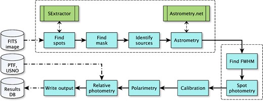
Flow chart representation of the operation of the pipeline. The FITS image from the CCD is first processed in a source identification step (Section 3.2), in which we match spots to sources in the sky and calculate their astronomical coordinates. We then perform photometry on all the identified sources (Section 3.3). The measured spot counts are corrected for instrumental errors in the calibration step (Section 3.4) before we measure the linear polarization (Section 3.5) and relative photometry (Section 3.6).
3.2 Source identification
Every point in the sky or focal plane is mapped to four points on the CCD by the RoboPol instrument. The first step in the pipeline is to identify which spots on the CCD correspond to which source in the sky, i.e. to reverse the 1↦4 mapping of the instrument.
We use SExtractor (Bertin & Arnouts 1996) to find the pixel coordinates of the centre of every spot on the CCD. After finding the location of the mask, and discarding spots whose photometry aperture is obscured by it, we find all sets of spots on the CCD that originate from the same astronomical source (described in Section 3.2.1 below).
We use the central point, defined as the intersection of the line that joins the vertical spots and the line that joins the horizontal spots, for each set of four spots to determine the WCS that describes the image using the astrometry.net (Lang et al. 2010) software. We then use this WCS to transform the central pixel coordinate for each set of four spots to a J2000 coordinate. The astrometry.net software bases its astrometry on index files that are calculated from either the USNO-B catalogue (Monet et al. 2003) or the 2MASS catalogue (Skrutskie et al. 2006); the RoboPol pipeline uses the 2MASS-derived index files5. We have found that the astrometry solutions for the target source are within 3 arcsec of the catalogue position 90 per cent of the time, independent of seeing conditions or position on the sky.
3.2.1 Spot matching method
A typical RoboPol exposure, such as the example shown in Fig. 2, contains a large number of sources in the field. Each source forms four corresponding spots on the CCD. We describe here a method for determining which spots on the CCD correspond to which source in the sky, i.e. a method for finding sets of four spots automatically. We use our knowledge of the expected spot pattern from the instrument model to do this.
Suppose we have found M spots on the CCD, with pixel coordinates (x1, y1), …, (xM, yM). For each spot, we can then use the instrument model (Section 2.2.1 and Appendix A) to predict the location of the intersection of the line joining the vertical spot pair and the line joining the horizontal spot pair, i.e. the central point. However, this requires us to know what type of spot each spot is, i.e. 0, 1, 2, or 3. Since we do not know this a priori, we calculate where the central point would be in each of these four cases, producing four potential central points for each spot arranged above, below, left, and right of the spot on the CCD.
We then have a set of 4M predicted central points. The four spots which correspond to a particular source will have the same predicted central point. We search the set of predicted central points for groups of four points that lie within a threshold of ∼ 3 pixels of each other, to account for centroid and model errors.
3.3 Photometry
After the spots have been detected and matched to sources in the sky, we measure the intensity of each spot using aperture photometry. We calculate the mean full width at half-maximum (FWHM) across the field using 10 spots that are bright, unblended, and unsaturated. We fit both a Gaussian and a Moffat profile (Moffat 1969), and use the FWHM estimate from the best-fitting profile.
3.3.1 Mask detection
We must find the exact location of the mask in order to perform aperture photometry on the central target, and to identify and reject sources whose photometric aperture intersects with the mask. We find the position of the mask by fitting the known mask pattern to the image. This is done by finding the mask pattern position that maximizes the difference in background level between stripes of pixels on either side of the mask pattern edge. Pixels contaminated by bright sources located near the mask pattern edge are excluded from the procedure.
Knowing the geometry of the mask, we can then identify the location of the low background areas, squares 22 arcsec × 22 arcsec in size in which the central target should be located. An image of the central area from a RoboPol image, with the mask pattern and low background areas outlined, is shown in Fig. 4. The mask detection is also used in the target acquisition procedure outlined in Section 4.3.
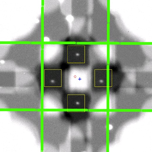
An image of the central area of the RoboPol field. The four low background areas due to the focal plane mask, containing the four spots of the central science target, are located in the centre of the field. The edges of the mask pattern are indicated in green. The yellow squares are the background estimation boxes for the central science target, the red diamond is the mask centre, and the blue cross is the pointing centre. Optical distortions result in the mask centre and pointing centre being slightly different: the pointing centre offset from the mask centre was determined empirically.
3.3.2 Aperture photometry
For the field sources, we use circular apertures centred on each spot to measure the intensity and an outer annulus to estimate the background level. We use the SExtractor positions of the spot centres, and flag blended spots (these are currently not analysed by the pipeline). The focal plane mask restricts the area around the central target that can be used to estimate the background level, so we use a square aperture, as indicated by the yellow boxes in Fig. 4, for the central target spots to maximize the number of pixels used in the background estimation. The location of the square apertures is set by the location of the mask, regardless of the location of the source spots.
We estimate the background level using a method outlined in Da Costa (1992). The background level is the mode of the smoothed distribution of all pixels that have an intensity within 3σ of the median level in the aperture.
We evaluated the performance of the RoboPol aperture photometry code by comparing its output to the output of the Aperture Photometry Tool (apt) software (Laher et al. 2012). We ran apt in batch mode on a set of RoboPol images. We fixed the photometry apertures used by apt to match those used by the RoboPol pipeline. The results are shown in Fig. 5, where we plot the relative difference between the RoboPol intensity and that obtained by apt. The apt and RoboPol results have excellent agreement, with a median relative difference of 0.04 per cent. The outlier points are due to errors in the background level estimation due to proximity of the source to the focal plane mask.
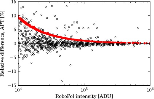
Comparison of the source intensity measured by the RoboPol pipeline with that measured by Aperture Photometry Tool (apt). The apt used the same aperture settings as used by the RoboPol pipeline. The median difference is 0.04 per cent. The red points are the 1σ uncertainties in the RoboPol intensities, calculated using Poisson statistics. The outlier points are sources close to the focal plane mask: the RoboPol pipeline removes pixels in the focal plane mask from the background estimation annulus, while apt does not.
3.4 Calibration
3.5 Polarimetry
We tested the performance of the RoboPol pipeline by observing a number of polarized standard stars with known polarization properties in the Johnson–Cousins R-band. The polarization standards we observed are listed in Table 1. In Fig. 6, we plot light curves of the difference between the polarization fraction measured by the RoboPol pipeline and the catalogue value, and the difference between the RoboPol polarization angle and the catalogue value. No de-biasing has been applied, as the SNR of each measurement is large (>20:1). There is no systematic difference between the RoboPol polarization percentage and the catalogue value: the mean difference in polarization percentage is (3 ± 5) × 10−2. The polarization angles measured by the RoboPol instrument are on average 2|$_{.}^{\circ}$|31 ± 0|$_{.}^{\circ}$|34 larger than the catalogue angle. This is due to a rotation of the telescope polarization reference frame with respect to the sky.
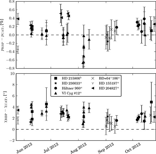
Light curves for a selection of polarization standard stars. We plot the difference between the RoboPol measured linear polarization percentage (pRBP) or angle (χRBP), and the catalogue value (pCAT, χCAT). The mean values for each standard are listed in Table 1, including references for the catalogue values.
Comparison of the RoboPol pipeline results for a set of polarized standard stars observed in the R-band (linear polarization percentage pRBP, σRBP, and position angle χRBP, σχ, RBP) and their catalogue values (subscript CAT). The values listed here are the unweighted means of the measurements shown in Fig. 6. Catalogue values are from: aSchmidt, Elston & Lupie (1992), bWhittet et al. (1992).
| Source . | pRBP (per cent) . | σp, RBP . | χRBP (°) . | σχ, RBP . | pCAT (per cent) . | σp, CAT . | χCAT (°) . | σχ, CAT . |
|---|---|---|---|---|---|---|---|---|
| VI Cyg #12a | 7.78 | 0.05 | 119.2 | 0.2 | 7.893 | 0.037 | 116.23 | 0.14 |
| HD 236633a | 5.22 | 0.23 | 95.4 | 1.3 | 5.376 | 0.028 | 93.04 | 0.15 |
| Hiltner 960a | 5.45 | 0.08 | 56.4 | 0.4 | 5.210 | 0.029 | 54.54 | 0.16 |
| BD+64°106a | 5.19 | 0.10 | 98.0 | 0.6 | 5.150 | 0.098 | 96.74 | 0.54 |
| HD 204827a | 5.29 | 0.06 | 61.6 | 0.3 | 4.893 | 0.029 | 59.10 | 0.17 |
| HD 155197a | 3.92 | 0.09 | 104.5 | 0.7 | 4.274 | 0.027 | 102.88 | 0.18 |
| HD 215806b | 1.96 | 0.09 | 69.6 | 1.3 | 1.830 | 0.040 | 66.00 | 1.00 |
3.6 Relative photometry
We measure the brightness of the objects in the RoboPol field relative to a set of non-variable reference sources in the field. This requires a reliable reference photometric catalogue. There are two catalogues that have significant overlap with our sources, the PTF (Palomar Transient Factory) R-band catalogue (Ofek et al. 2012b) and the USNO-B1.0 catalogue (Monet et al. 2003). However, we have found the USNO-B1.0 magnitudes to be unsuitable for use as photometric standards due to their marginal photometric quality.
We identify all reference sources in the RoboPol frame that are uncontaminated, i.e. that are not blended sources and that do not have any sources in their background estimation annulus. We find their catalogue magnitude and convert it to a flux using the zero-point for the Johnson–Cousins photometric system. We find the best-fitting line to the total source intensity (sum of the four spot intensities |$\sum _{i=1}^{4}N_{i}^{c}$|) versus flux for the reference sources, and use this relationship to convert the total intensity for all the sources in the frame to an R-band magnitude. We measure the standard deviation of the difference between the RoboPol magnitude and the catalogue magnitude for the reference sources, and call this the ‘standards’ uncertainty. This systematic uncertainty is the same for every source in the field. The uncertainty in the magnitude of a source is then the quadrature sum of the statistical uncertainty for that source (SNR in intensity measurement) and the ‘standards’ uncertainty.
In Fig. 7, we show the distribution of the difference between the RoboPol R-band magnitude and the PTF catalogue R-band magnitude (corrected using equation 9) for a set of RoboPol field sources. The magnitudes are very similar, and the scatter in the difference is consistent with that expected from the SNR in the spot photometry measurement.
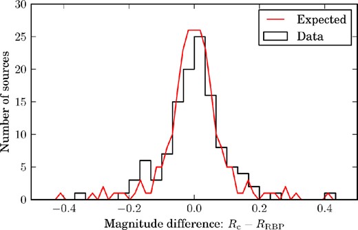
Distribution of the difference between the RoboPol-measured R-band magnitude RRBP and the PTF R-band magnitude (corrected using equation 9) Rc. The red curve shows the distribution of the expected magnitude uncertainty calculated as |$R_{\rm RBP}\frac{\sigma _N}{N}$| (where N is the source intensity and σN is its uncertainty), mirrored around 0. The difference in the magnitudes is consistent with the level expected from photon counting statistics; no systematic difference is evident.
4 CONTROL SYSTEM
4.1 Overview
The RoboPol control system is designed with high observing efficiency and dynamic scheduling as prime goals. High efficiency is achieved by full automation of the observing process, and dynamic adjustment of the exposure time for a target to reach a specified SNR goal.
The control system operates the Skinakas 1.3-m telescope robotically during RoboPol observing sessions, and allows full manual control of the telescope the rest of the time. As described in Section 2.1, the control of the telescope subsystems is spread over several computers running a variety of operating systems. The RoboPol control system is written in python and consists of a number of independent processes running on these computers, communicating with each other over ethernet using TCP sockets.
A simplified flow chart of the main observing loop in the master control process is shown in Fig. 8. Some of the other independent processes are shown in purple. The control system processes are as follows.
Master: control the observing process.
Scheduler: provide the next object to observe (Section 4.2).
Pipeline queue: analyse the FITS images from the instrument and provide the science target magnitude and linear polarization to the master and scheduler processes.
Gamma-ray data pipeline (not shown): process the gamma-ray data provided by the Fermi large area telescope (LAT) offline and provide the latest data to the scheduler process.
Telescope control: interface with the mount, dome, and focus control through the TCS computer, control of the RoboPol filter wheel and CCD.
GUI (not shown): a graphical interface to the control system to provide the telescope operator with feedback and allow manual intervention if necessary.
Weather (not shown): monitor a weather station to provide information to the watchdog processes and for logging.
Watchdogs (not shown): monitor and maintain the stability of the control system.
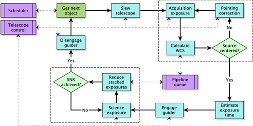
Flow chart representation of the main observing loop. The observing loop gets the next object from the scheduler process (Section 4.2) and instructs the telescope control process to slew to the target. A target acquisition loop (Section 4.3) then ensures that the science target is centred in the mask. The source is then observed until the SNR goal is reached (Section 4.4). The loop then acquires the next object from the observing queue.
In addition to the fully automated main observing loop, the control system runs an automated focus routine (Section 4.5) several times during the night, automatically acquires flat-field exposures (Section 4.6) to monitor dust contamination of the optics, and has a target-of-opportunity mode that can interrupt the main observing loop to observe, for instance, gamma-ray burst optical afterglows.
All exposures made by the control system are stored on disc at the telescope and transferred once a day to servers at the University of Crete. From there the data are distributed over the internet to the partner institutions for redundant backup. A data base of light curves for all the sources in every RoboPol field is maintained at the University of Crete.
4.2 Dynamic scheduling
The RoboPol control system is designed to allow dynamic scheduling. At the start of each night the scheduler process produces a nominal schedule of the sources from the RoboPol catalogue that are due to be observed. As each source is observed its measured magnitude and linear polarization are passed to the scheduler process to allow changes to the schedule to be made, if necessary. This dynamic response mode is not being used in the first observing season while we gather the data necessary to characterize the behaviour of our sources and develop the algorithms to reliably identify interesting behaviour. Details of the dynamical scheduler will be reported in future papers.
4.3 Target acquisition
The pointing requirements for the RoboPol instrument are very stringent: we require the science target to be within 2 arcsec of the pointing centre of the mask. We cannot achieve this precision with a blind slew to a source, so the control system contains a target acquisition loop to centre the source in the mask before taking the science exposures.
After the initial telescope slew, the control system takes a short exposure of the field. This is processed using the pipeline to find the mask location and to calculate the WCS that describes the frame. A pointing correction that would place the target coordinates at the mask pointing centre is calculated. This correction is applied and another short exposure is taken. This loop is repeated until the target source is properly located. The performance of the target acquisition system is shown in Fig. 9. Most initial slews are within ∼2 arcmin of the commanded position, and ∼90 per cent of sources require two or fewer pointing corrections to be properly placed in the mask.
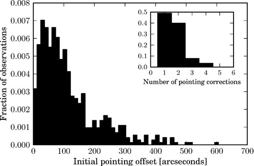
The initial pointing offset of the field centre from the commanded position. Inset: about 90 per cent of sources require two or fewer pointing corrections to be properly centred.
It is not necessary for the central target source to be visible in a single exposure for this procedure to work. As long as there are enough stars in the field for the pipeline to calculate the WCS for the frame, the location of the source in the field can be calculated and the appropriate pointing correction applied.
4.4 Dynamic exposure time
Both the polarization and magnitude of blazars are highly variable at optical wavelengths. For greater observing efficiency, we expose only long enough to reach a target SNR of 10:1 in p, which equates to an uncertainty in the EVPA of ∼2|$_{.}^{\circ}$|86 (see equation 7). Because the blazar emission can change significantly from night to night (and even within a night), we calculate the necessary exposure time to reach our SNR goal from the data as we gather it.
We use the final target acquisition exposure to provide an initial guess for the required exposure time. We calculate the amount of time needed to collect 250 000 photons in total from the source, which we have found gives an SNR in p of ∼10:1 in an ∼3 per cent polarized source under average observing conditions at Skinakas. We then take a number of science exposures; as the science exposures are accumulated we run the pipeline on the stacked image and update the estimate of the required observing time. We stop observing once the SNR goal is reached, or when the total exposure time has reached 40 min.
4.5 Autofocus
The RoboPol instrument is optimized to measure the linear polarization of point sources. The control system contains an autofocus mode that takes a series of exposures at different focus positions. It then finds the focus position that produces the lowest median FWHM across the field. While the FWHM does vary across the field, the minimum in the median FWHM corresponds to the same focal position as the minimum in the FWHM of the central target, and the curve of median FWHM versus focus position has lower noise than the curve for a single source. This procedure is run at the beginning and mid-way through each night.
4.6 Autoflats
The control system automatically takes flat-field exposures at dawn or dusk, which are used to track the presence of dust in the telescope optics and its effect on the performance of the instrument.
We select an observing location for the flat-field exposures by requiring that the distance of the target flat-field sky area from the Moon be more than 50° and that the distance from the horizon be more than 40°, thereby limiting the gradient of the background to <1 per cent across our field (Chromey & Hasselbacher 1996). The control system selects as the target sky area the point on the line of declination δ = +32° that meets these criteria and has the greatest summed distance from the Moon and the horizon.
According to Tyson & Gal (1993) the logarithm of the brightness of the sky changes linearly with time, with possible deviations due to atmospheric dust. We have found that the sky brightness light curve is better described by a second-order polynomial. We take a series of short exposures of the sky every 120 s to characterize the median sky brightness light curve. Once the changing sky brightness is adequately characterized, we calculate the optimum time to start taking the flat-field exposures such that we get a median background count of ∼10 000 ADU pixel−1 (∼1/3 of the non-linear point for this CCD) in the first flat-field exposure. We then take a series of 3-10 s exposures while varying the pointing location of the telescope, which is used to calculate the master flat-field image.
5 CONCLUSIONS
We have described the data reduction pipeline and control system developed for the RoboPol project. We have shown that the aperture photometry using circular apertures performed by the RoboPol pipeline produces results that are indistinguishable from those obtained using the standard apt (Laher et al. 2012). Our aperture photometry code has a substantially faster processing time than apt, though it should be noted that apt was not designed with processing speed as a primary goal. By using our own code, we are also able to use a square background estimation aperture for the central target, thereby taking full advantage of the focal plane mask.
Most optical polarimeters use a rotating polarization element to remove instrumental effects from the polarization measurement. The RoboPol instrument does not; we instead take a single exposure and use a model of the instrumental effects (Appendix A) to correct the measured spot intensities before calculating the source polarization. The instrument model is derived from observations of unpolarized standard stars at multiple locations in the RoboPol field of view. We used the RoboPol pipeline to analyse observations of a set of polarized standard stars and found that the measured polarizations matched the catalogue polarizations to within the statistical error.
The measurement of the magnitude of the sources in a RoboPol image is obtained by relative photometry against photometric standards in the field. The only catalogue of photometric standards of sufficient quality and sky coverage to be suitable for use with the RoboPol data is the PTF R-band catalogue (Ofek et al. 2012b). However, it does not include the fields around every source in the RoboPol sample and is not in the same photometric system as the RoboPol data, so we are in the process of taking the necessary data to extend the PTF R-band catalogue to cover all RoboPol sources in the Johnson–Cousins photometric system. All the RoboPol data will be reprocessed using our new catalogue of standards once it is complete. We have shown that the magnitudes measured by the RoboPol pipeline are consistent with those in the PTF catalogue.
The RoboPol control system is written to allow dynamic scheduling. It analyses each image as it is taken and sends the results to the scheduler. A primary goal of the RoboPol project is to use this information to respond immediately to important changes in a source's behaviour without human intervention. However, knowing what changes in a source's emission are important requires us to first characterize their behaviour. In the first observing season, we are taking the data necessary to perform this characterization, and will report on the resulting design of the dynamical scheduler in future papers. Due to the modular design of the RoboPol control system we will be able to change the scheduling code with minimal effort.
The RoboPol project is a collaboration between Caltech in the USA, MPIfR in Germany, Toruń Centre for Astronomy in Poland, the University of Crete/FORTH in Greece, and IUCAA in India. The University of Crete group acknowledges support by the ‘RoboPol’ project, which is implemented under the ‘Aristeia’ Action of the ‘Operational Programme Education and Lifelong Learning’ and is co-funded by the European Social Fund (ESF) and Greek National Resources, and by the European Commission Seventh Framework Programme (FP7) through grants PCIG10-GA-2011-304001 ‘JetPop’ and PIRSES-GA-2012-31578 ‘EuroCal’. This research was supported in part by NASA grant NNX11A043G and NSF grant AST-1109911, and by the Polish National Science Centre, grant number 2011/01/B/ST9/04618. KT acknowledges support by the European Commission Seventh Framework Programme (FP7) through the Marie Curie Career Integration Grant PCIG-GA-2011-293531 ‘SFOnset’. MB acknowledges support from the International Fulbright Science and Technology Award. TH was supported in part by the Academy of Finland project number 267324. This research made use of astropy, http://www.astropy.org, a community-developed core python package for astronomy (Astropy Collaboration 2013). IM is supported for this research through a stipend from the International Max Planck Research School (IMPRS) for Astronomy and Astrophysics at the Universities of Bonn and Cologne.
Downloaded from http://data.astrometry.net/4200/
REFERENCES
APPENDIX A: INSTRUMENT MODEL
The instrument model describes two separate behaviours of the RoboPol receiver. These are the variation in the spatial pattern made by the spots on the CCD, and the effect on the intensity of each spot. The data used to generate the model come from a series of exposures of a standard unpolarized star. In each exposure, the telescope pointing is stepped by 1 arcmin, thereby sampling a grid of points in the field of view with the standard source. Fig. A1 shows the locations of the standard star in a series of such exposures.
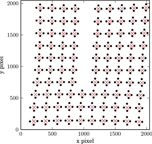
A plot showing the location of the standard unpolarized star HD 154892 in a series of exposures. The individual spots are indicated by black dots, and the central point by a red cross.
Since the intrinsic magnitude and polarization of the source does not change over the course of the exposures, any changes in the observed magnitude or polarization of the source are due to aberrations in the combined telescope and instrument optics. We can then model the corrections to the spot intensities that will result in a source of zero polarization and constant magnitude regardless of where in the field of view it is located.
The model described here is agnostic about the source of the aberrations that it corrects for. It is purely empirical: it corrects for the observed behaviour with as few parameters as necessary, regardless of the physical source of the aberrant behaviour. The functional forms used in the model were selected by best fit to the data, rather than derived from a physical model of the optics.
A1 Spatial model
The spatial model predicts the location of the four spots on the CCD, given the location of the source (x, y). As shown in Fig. 1, this pattern is described by six numbers. The distance between the horizontal spots is given by Δx(x, y), and between the vertical spots it is Δy(x, y). The distance from the right-spot to the central point (x, y) is given by δx(x, y), and from the upper-spot it is δy(x, y). Finally, the angle between the CCD x-axis and the horizontal line is ϕx(x, y) and the angle between the CCD y-axis and the vertical line is ϕy(x, y).

The data (left), best-fitting model (centre), and residuals (right) for the quantity Δx in the instrument spatial pattern model. Note the change in colour scale for the residual plot. Areas in the plot with no data, due to imperfect coverage of the field as shown in Fig. A1, are blank.

The data (left), best-fitting model (centre), and residuals (right) for the quantity δx in the instrument spatial pattern model. Note the change in colour scale for the residual plot.

The data (left), best-fitting model (centre), and residuals (right) for the quantity ϕx in the instrument spatial pattern model. Note the change in colour scale for the residual plot.
The best-fitting model for each case are shown in the centre panel of Figs A2–A4, and the residual (difference between the data and the model in each cell) is shown in panel (c). The fits are generally excellent, with the residuals for the δ parameters being noise dominated. Some coherent structure remains in the residuals for the Δ and ϕ quantities, but the level of the residuals are low enough that the spot matching method described in Section 3.2.1 works, and there is hence no need to add additional detail to the model.
A2 Intensity model
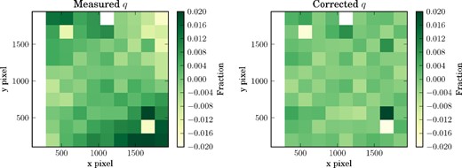
The uncorrected (left) and corrected (right) relative Stokes q parameter, which correspond to before and after applying the instrument intensity model to the data, respectively.
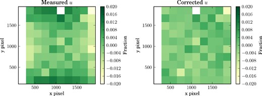
The uncorrected (left) and corrected (right) relative Stokes u parameter, which correspond to before and after applying the instrument intensity model to the data, respectively.
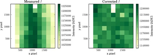
The uncorrected (left) and corrected (right) total source intensity, which correspond to before and after applying the instrument intensity model to the data, respectively. Note the change in colour scale for the corrected plot.


